
The Influence of Instrumental Line Shape Degradation on Gas Retrievals and Observation of Greenhouse Gases in Maoming, China


Abstract
:1. Introduction
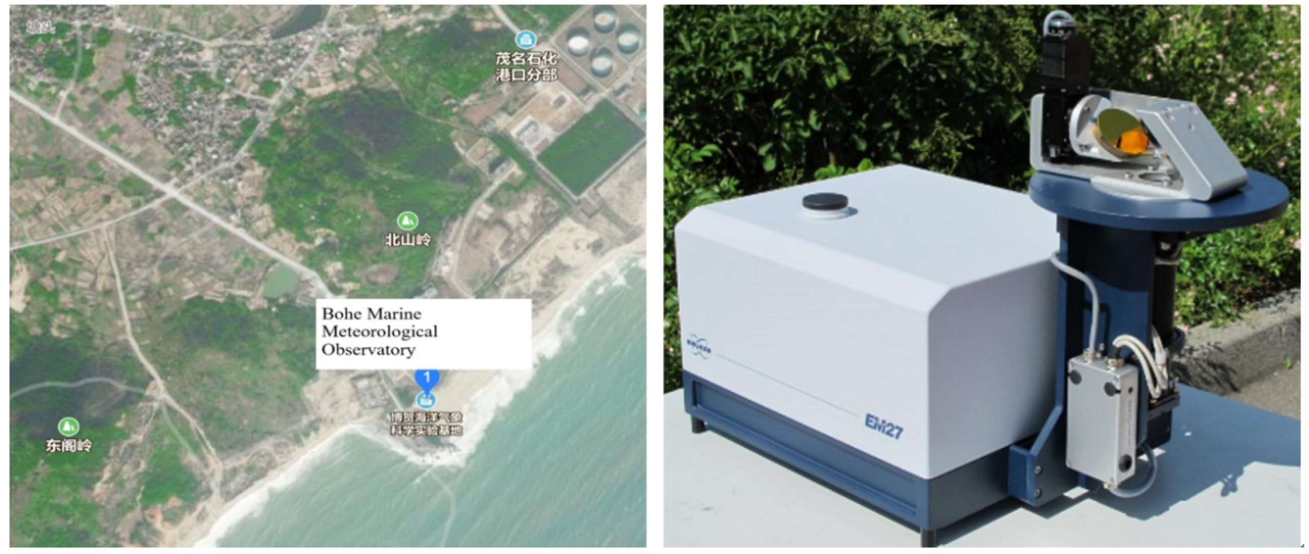
2. Measurement Sit and Instruments
3. Data Processing and Methods
4. Results Measurements and Discussion
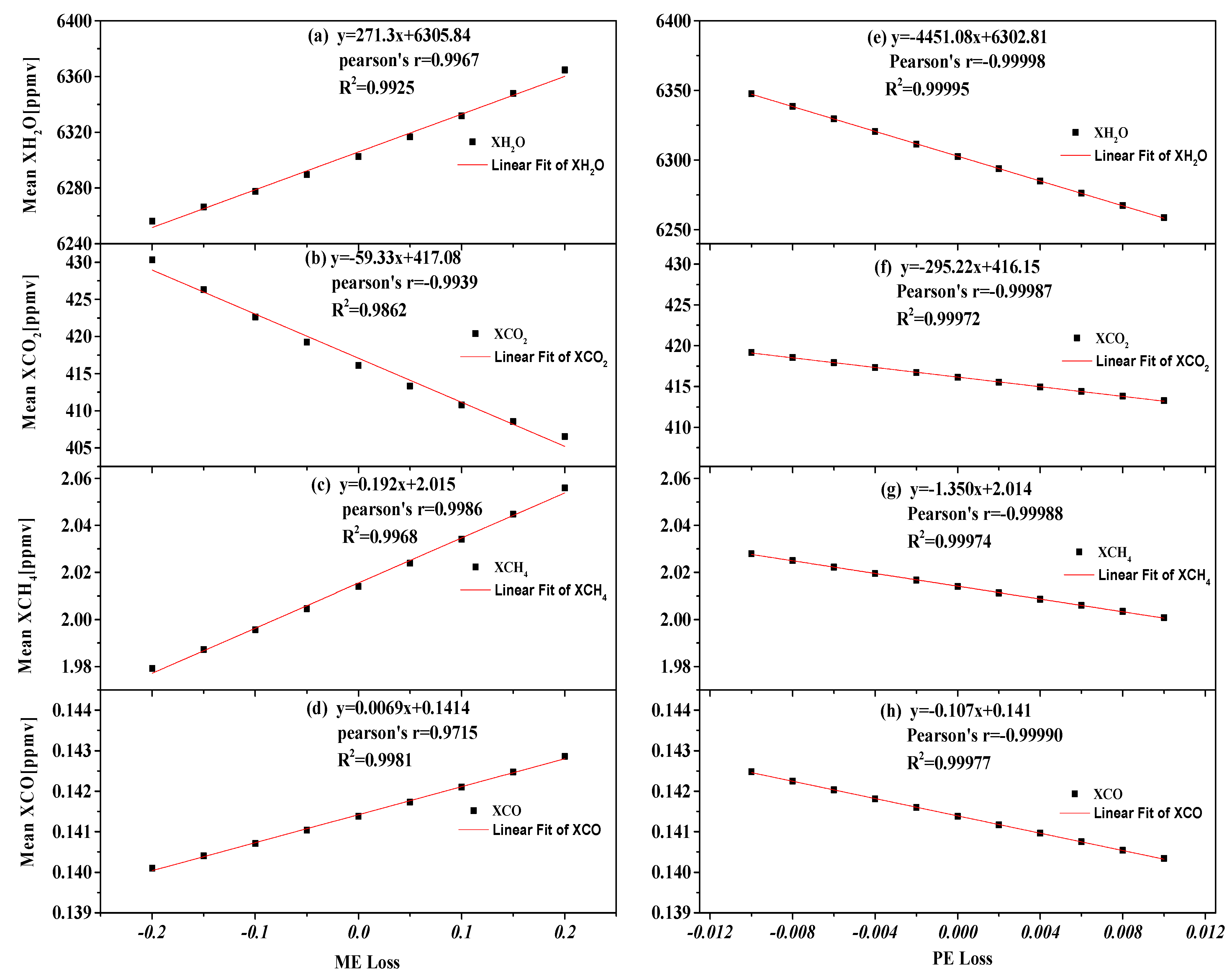
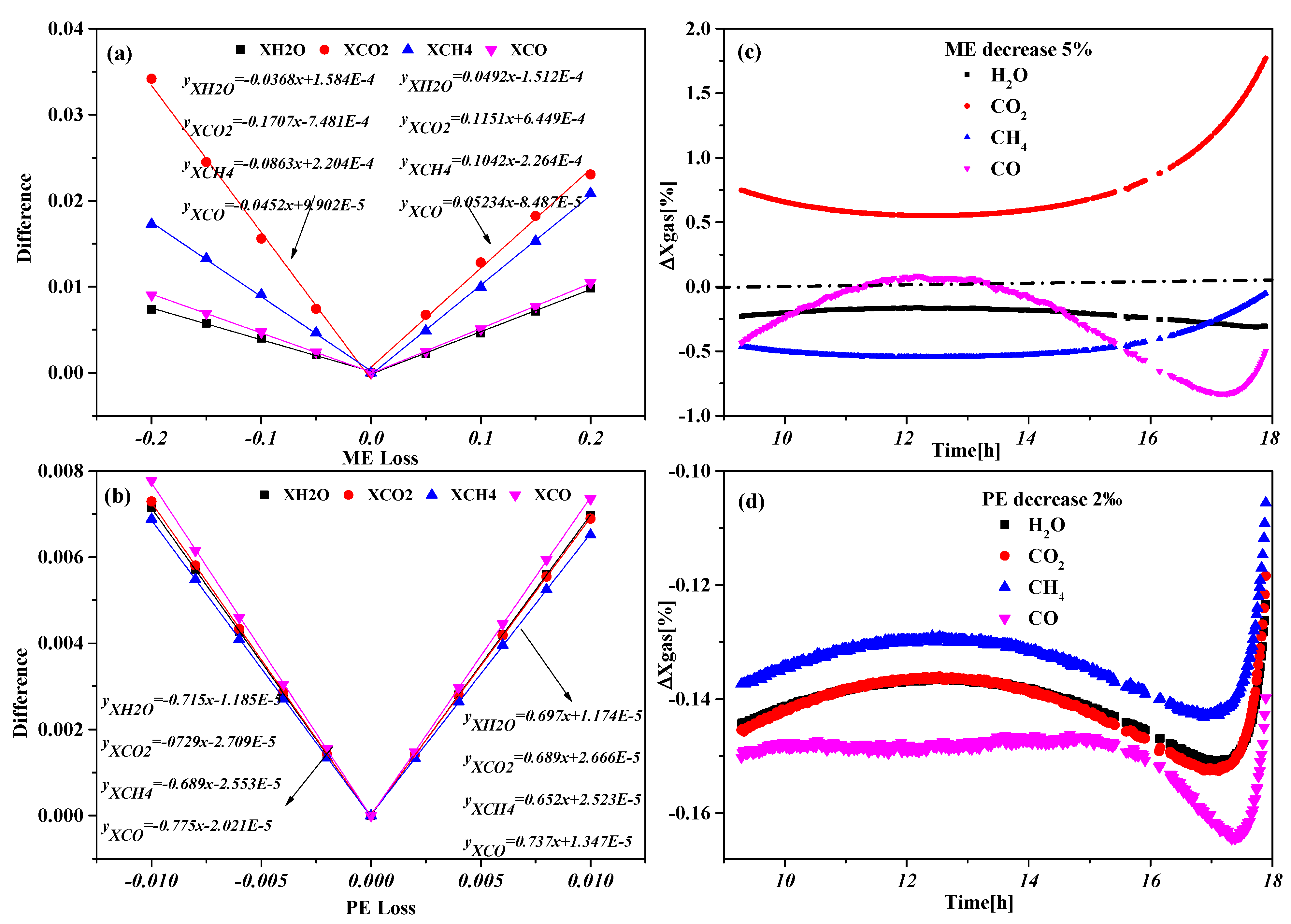
4.1. Influence of Instrumental Line Shape on Greenhouse Gas Inversion
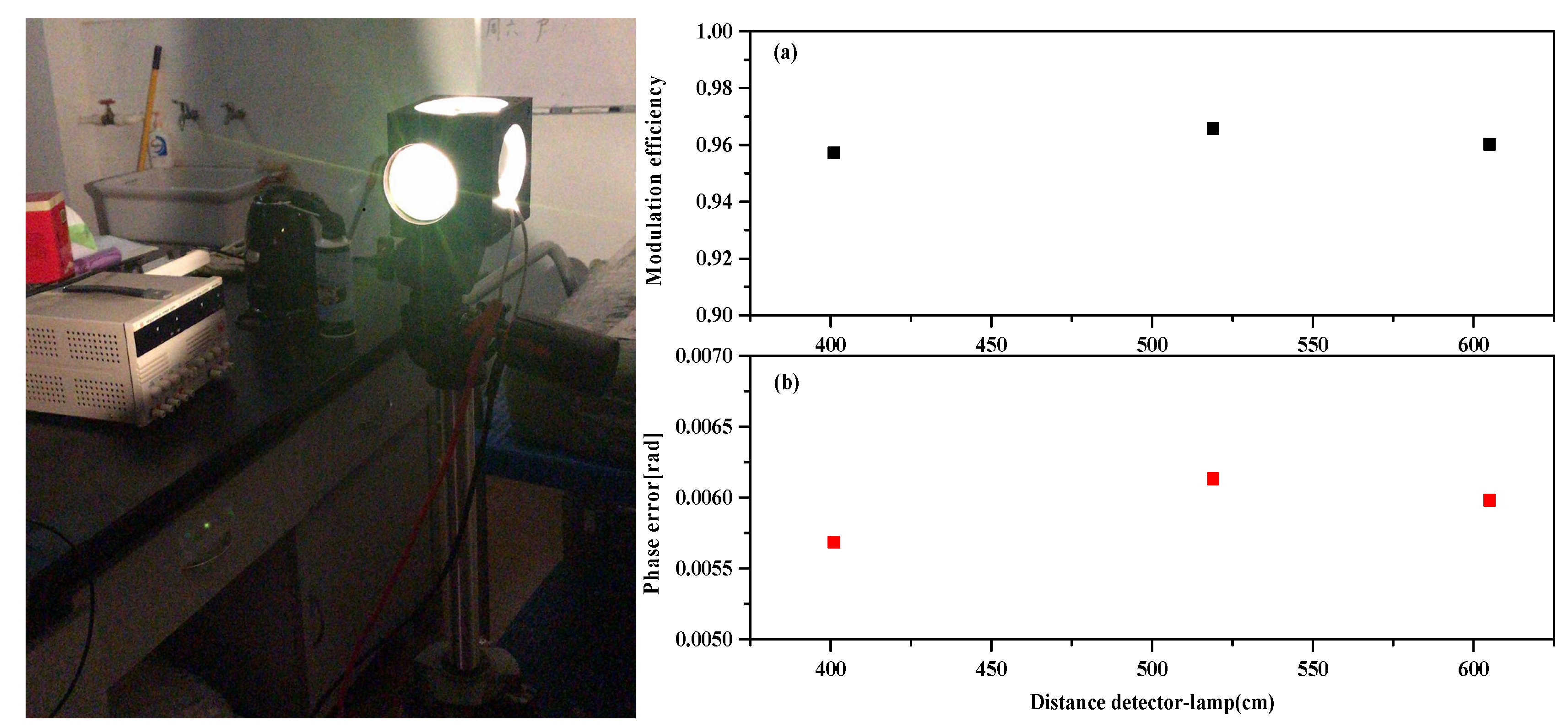
4.2. Instrumental Line Shape Monitoring
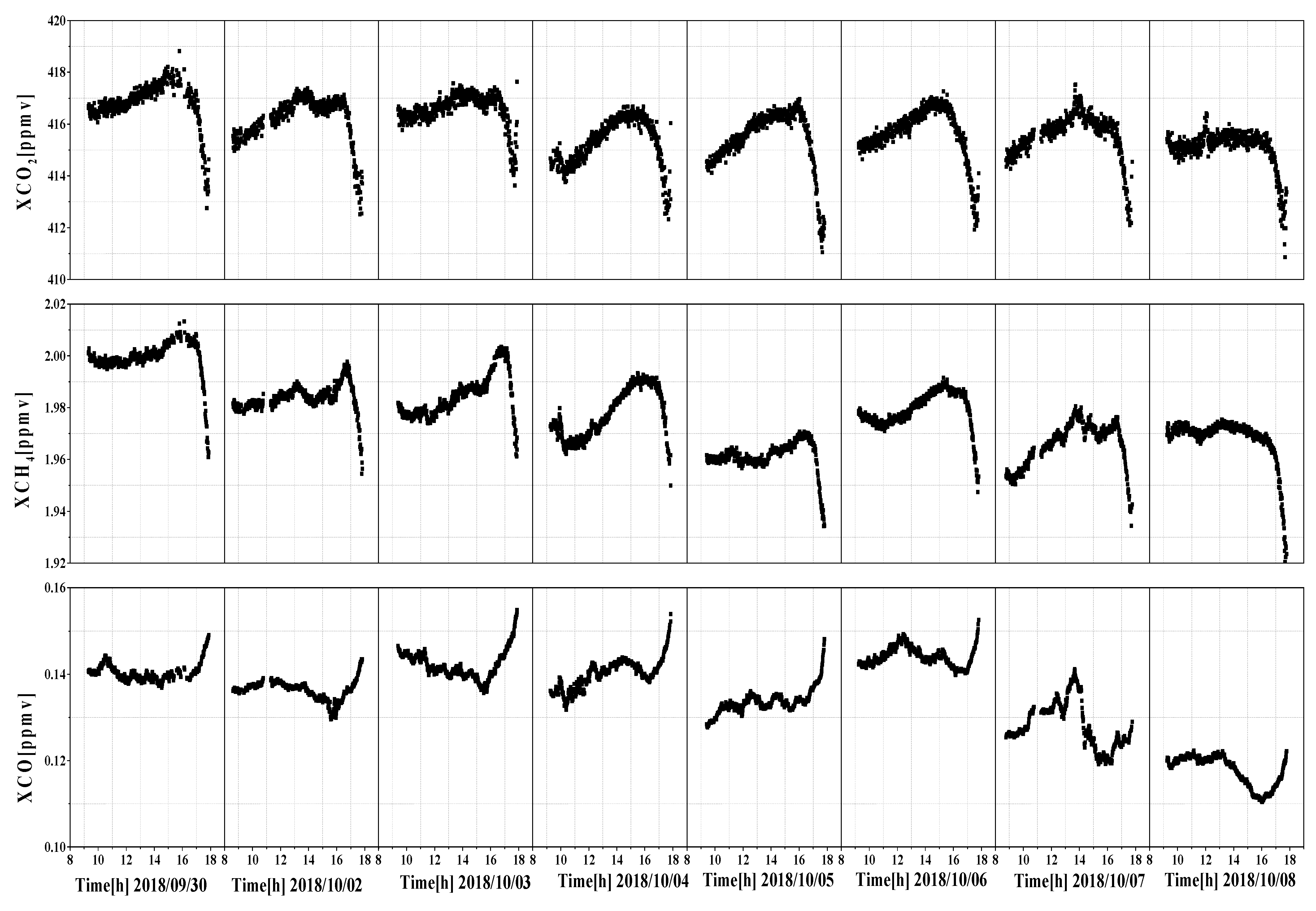
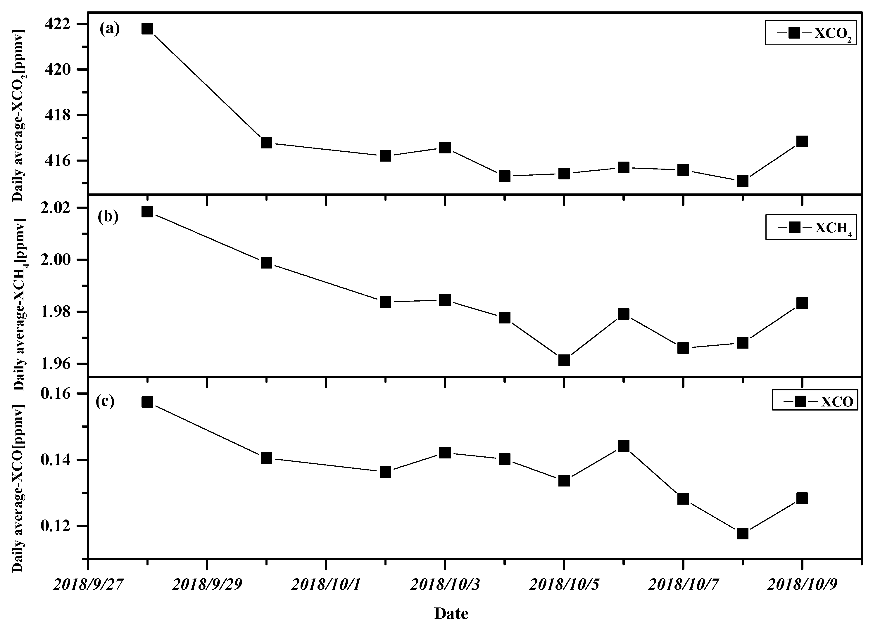
4.3. Variation of XCO2, XCH4 and XCO
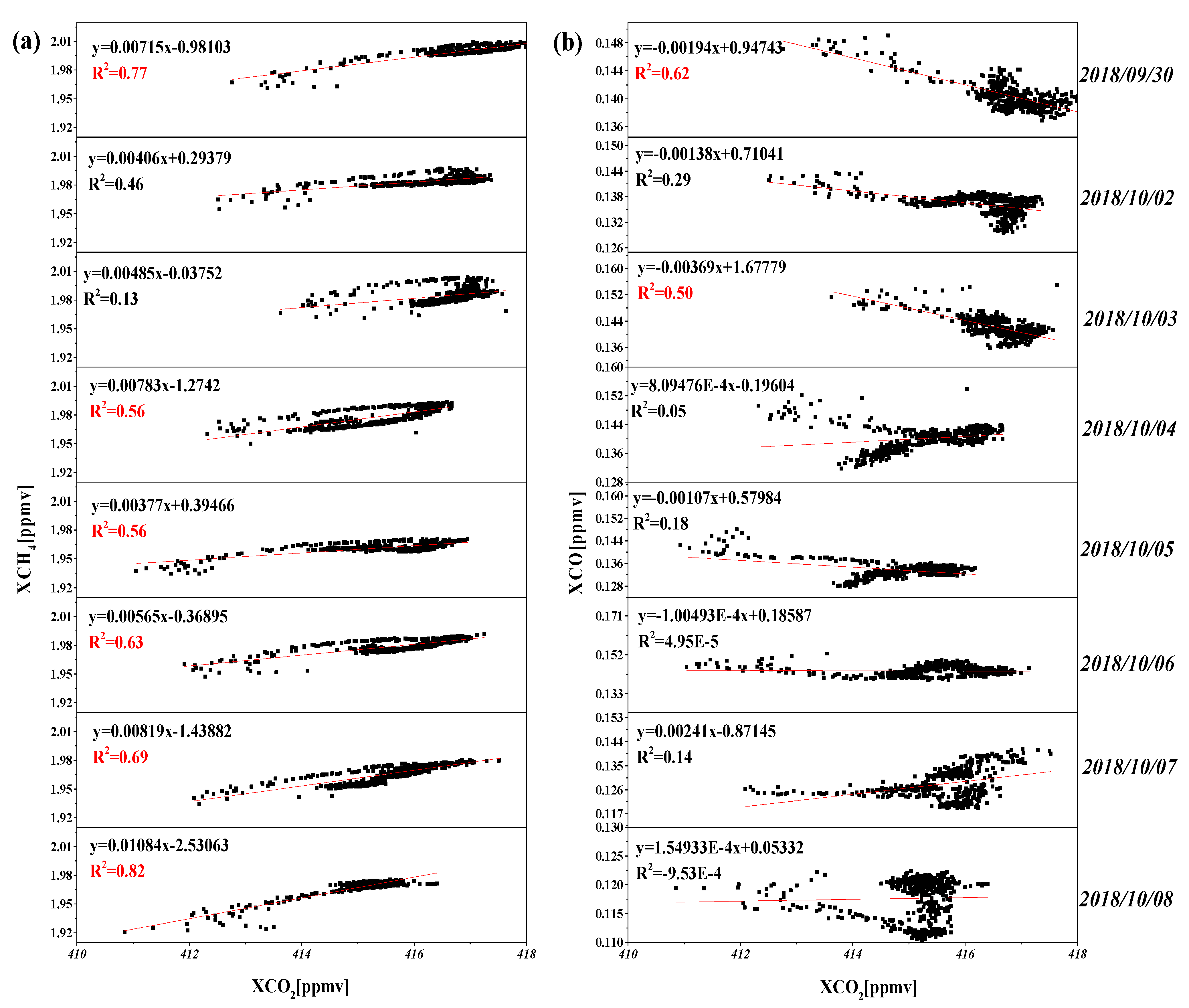
4.4. The Correlation between XCH4, XCO, and XCO2
5. Conclusions
Author Contributions
Funding
Institutional Review Board Statement
Informed Consent Statement
Data Availability Statement
Acknowledgments
Conflicts of Interest
References
- Janardanan, R.; Maksyutov, S.; Oda, T.; Saito, M.; Kaiser, J.W.; Ganshin, A.; Stohl, A.; Matsunaga, T.; Yoshida, Y.; Yokota, T. Comparing GOSAT observations of localized CO2 enhancements by large emitters with inventory based estimates. Geophys. Res. Lett. 2016, 43, 3486–3493. [Google Scholar] [CrossRef] [Green Version]
- O’Brien, D.M.; Polonsky, I.N.; Utembe, S.R.; Rayner, P.J. Potential of a geostationary geoCARB mission to estimate surface emissions of CO2, CH4 and CO in a polluted urban environment: Case study Shanghai. Atmos. Meas. Tech. 2016, 9, 4633–4654. [Google Scholar] [CrossRef] [Green Version]
- Schwandner, F.M.; Gunson, M.R.; Miller, C.E.; Carn, S.A.; Eldering, A.; Krings, T.; Verhulst, K.R.; Schimel, D.S.; Nguyen, H.M.; Crisp, D.; et al. Spaceborne detection of localized carbon dioxide sources. Science 2017, 358, eaam5782. Available online: https://science.sciencemag.org/content/358/6360/eaam5782 (accessed on 5 May 2021). [CrossRef] [PubMed] [Green Version]
- Broquet, G.; Bréon, F.M.; Renault, E.; Buchwitz, M.; Reuter, M.; Bovensmann, H.; Chevallier, F.; Wu, L.; Ciais, P. The potential of satellite spectro-imagery for monitoring CO2 emissions from large cities. Atmos. Meas. Tech. 2018, 11, 681–708. [Google Scholar] [CrossRef] [Green Version]
- Wunch, D.; Toon, G.C.; Blavier, J.F.L.; Washenfelder, R.A.; Notholt, J.; Connor, B.J.; Griffith, D.W.T.; Sherlock, V.; Wennberg, P.O. The total carbon column observing network. Phil. Trans. R.Soc. A 2011, 369, 2087–2112. [Google Scholar] [CrossRef] [PubMed] [Green Version]
- Kurylo, M.J. Network for the detection of stratospheric change. Proc. SPIE 1991, 1491, 168–174. [Google Scholar] [CrossRef] [Green Version]
- Messerschmidt, J.; Geibel, M.C.; Blumenstock, T.; Chen, H.; Deutscher, N.M.; Engel, A.; Feist, D.G.; Gerbig, C.; Gisi, M.; Hase, F.; et al. Calibration of TCCON column-averaged CO2: The first aircraft campaign over European TCCON sites. Atmos. Chem. Phys. 2011, 11, 10765–10777. [Google Scholar] [CrossRef] [Green Version]
- Gisi, M.; Hase, F.; Dohe, S.; Blumenstock, T.; Simon, A.; Keens, A. XCO2-measurements with a tabletop FTS using solar absorption spectroscopy. Atmos. Meas. Tech. 2012, 5, 2969–2980. [Google Scholar] [CrossRef] [Green Version]
- Hase, F.; Frey, M.; Blumenstock, T.; Groß, J.; Kiel, M.; Kohlhepp, R.; Mengistu Tsidu, G.; Schäfer, K.; Sha, M.K.; Orphal, J. Application of portable FTIR spectrometers for detecting greenhouse gas emissions of the major city Berlin. Atmos. Meas. Tech. 2015, 8, 3059–3068. Available online: https://amt.copernicus.org/articles/8/3059/2015/amt-8-3059-2015 (accessed on 5 May 2021). [CrossRef] [Green Version]
- Frey, M.; Hase, F.; Blumenstock, T.; Groß, J.; Kiel, M.; Tsidu, G.M.; Schäfer, K.; Sha, M.K.; Orphal, J. Use of portable FTIR spectrometers for detecting greenhouse gas emissions of the megacity Berlin–Part 1: Instrumental line shape characterisation and calibration of a quintuple of spectrometers. Atmos. Meas. Tech. 2015, 8, 3047–3057. [Google Scholar] [CrossRef] [Green Version]
- Frey, M. Characterisation and Application of Portable Solar Absorption Spectrometers for the Detection of Greenhouse Gas Emissions from Regional Anthropogenic Sources. Ph.D. Thesis, Karlsruhe Institute for Technolgy (KIT), Karlsruhe, Germany, 2018. [Google Scholar]
- Klappenbach, F.; Bertleff, M.; Kostinek, J.; Hase, F.; Blumenstock, T.; Agusti-Panareda, A.; Razinger, M.; Butz, A. Accurate mobile remote sensing of XCO2 and XCH4 latitudinal transects from aboard a research vessel. Atmos. Meas. Tech. 2015, 8, 5023–5038. [Google Scholar] [CrossRef] [Green Version]
- Norton, R.H.; Beer, R. New apodizing functions for Fourier spectrometry. J. Opt. Soc. Am. 1976, 67, 419. Available online: https://www.researchgate.net/publication/23822078_New_apodizing_functions_for_Fourier_spectrometry (accessed on 5 May 2021). [CrossRef]
- Davis, S.P.; Abrams, M.C.; Brault, J.W. Fourier Transform Spectrometry; Academic Press: Cambridge, MA, USA, 2001; ISBN 0-12-042510-6. [Google Scholar]
- Hase, F.; Blumenstock, T.; Paton-Walsh, C. Analysis of the instrumental line shape of high resolution Fourier transform IR spectrometers with gas cell measurements and new retrieval software. Appl. Opt. 1999, 38, 3417–3422. [Google Scholar] [CrossRef] [PubMed]
- Kiel, M.; Wunch, D.; Wennberg, P.O.; Toon, G.C.; Hase, F.; Blumenstock, T. Improved retrieval of gas abundances from near-infrared solar FTIR spectra measured at the Karlsruhe TCCON station. Atmos. Meas. Tech. 2016, 9, 669–682. [Google Scholar] [CrossRef] [Green Version]
- Frey, M.; Sha, M.K.; Hase, F.; Kiel, M.; Blumenstock, T.; Harig, R.; Surawicz, G.; Deutscher, N.M.; Shiomi, K.; Franklin, J.; et al. Building the Collaborative Carbon Column Observing Network (COCCON): Long-term stability and ensemble performance of the EM27/SUN Fourier transform spectrometer. Atmos. Meas. Tech. 2019, 12, 1513–1530. [Google Scholar] [CrossRef] [Green Version]
- Rodgers, C.D.; Connor, B.J. Intercomparison of remote sounding instruments. J. Geophys. Res. Atmos. 2003, 108. [Google Scholar] [CrossRef] [Green Version]
- Hedelius, J.K.; Viatte, C.; Wunch, D.; Roehl, C.M.; Toon, G.C.; Chen, J.; Jones, T.; Wofsy, S.C.; Franklin, J.E.; Parker, H.; et al. Assessment of errors and biases in retrievals of XCO2, XCH4, XCO, and XN2O from a 0.5 cm−1 resolution solar viewing spectrometer. Atmos. Meas. Tech. 2016, 9, 3527–3546. [Google Scholar] [CrossRef] [Green Version]
- Macdonald, J.; Fowler, D.; Hargreaves, K.; Skiba, U.; Leith, I.; Murray, M. Methane emission rates from a northern wetland; response to temperature, water table and transport. Atmos. Environ. 1998, 32, 3219–3227. [Google Scholar] [CrossRef]
- Denman, K.; Brasseur, G.P.; Chidthaisong, A.; Ciais, P.; Cox, P.M.; Dickinson, R.; Haugustaine, D.; Heinze, C.; Holland, E.A.; Jacob, D.; et al. Couplings between changes in the climate system and biogeochemistry. In Climate Change 2007: The Physical Science Basis. Contribution of Working Group I to the Fourth Assessment Report of the Intergovernmental Panel on Climate Change; Solomon, S., Qin, D., Manning, M., Chen, Z., Marquis, M., Averyt, K.B., Tignor, M., Miller, H.L., Eds.; Cambridge University Press: Cambridge, UK, 2007; pp. 499–587. [Google Scholar]
- Montzka, S.; Fraser, P.J.; Butler, J.H.; Cunnold, D.M.; Daniel, J.S.; Derwent, R.G.; Lal, S.; McCulloch, A.; Oram, D.E.; Reeves, C.E.; et al. Controlled substances and other source gases, Chapter 1 of the Scientific Assessment of Ozone Depletion: 2002. In Scientific Assessment of Ozone Depletion: 2002; World Meteorological Organization: Geneva, Switzerland, 2003; Volume 47, pp. 1.1–1.83. [Google Scholar]
- Fang, S.X.; Tans, P.P.; Steinbacher, M.; Zhou, L.X.; Luan, T. Comparison of the regional CO2 mole fraction filtering approaches at a WMO/GAW regional station in China. Atmos. Meas. Tech. 2015, 8, 5301–5313. [Google Scholar] [CrossRef] [Green Version]
- Turnbull, J.C.; Miller, J.B.; Lehman, S.J.; Tans, P.P.; Sparks, R.J.; Southon, J. Comparison of 14CO2, CO, and SF6 as tracers for recently added fossil fuel CO2 in the atmosphere and implications for biological CO2 exchange. Geophys. Res. Lett. 2006, 33, L01817. [Google Scholar] [CrossRef]
- Wang, Y.; Munger, J.W.; Xu, S.; McElroy, M.B.; Hao, J.; Nielsen, C.P.; Ma, H. CO2 and its correlation with CO at a rural site near Beijing: Implications for combustion efficiency in China. Atmos. Chem. Phys. 2010, 10, 8881–8897. [Google Scholar] [CrossRef] [Green Version]
- Wunch, D.; Wennberg, P.O.; Toon, G.C.; Keppel-Aleks, G.; Yavin, Y.G. Emissions of greenhouse gases from a North American megacity. Geophys. Res. Lett. 2009, 36, L15810. [Google Scholar] [CrossRef] [Green Version]
- Wang, W.; Tian, Y.; Liu, C.; Sun, Y.; Liu, W.; Xie, P.; Liu, J.; Xu, J.; Morino, I.; Voltaire, A.; et al. Investigating the performance of a greenhouse gas observatory in Hefei, China. Atmos. Meas. Tech. 2017, 10, 2627–2643. [Google Scholar] [CrossRef] [Green Version]
- Draxler, R.R.; Hess, G.D. An overview of the HYSPLIT 4 modeling system for trajectories, dispersion, and deposition. Aust. Met. Mag. 1998, 47, 295–308. [Google Scholar]


| Gas | Spectral Windows [cm−1] | Interfering Molecule |
|---|---|---|
| CO2 | 6173.0–6390.0 | H2O, HDO, CH4 |
| CH4 | 5897.0–6145.0 | H2O |
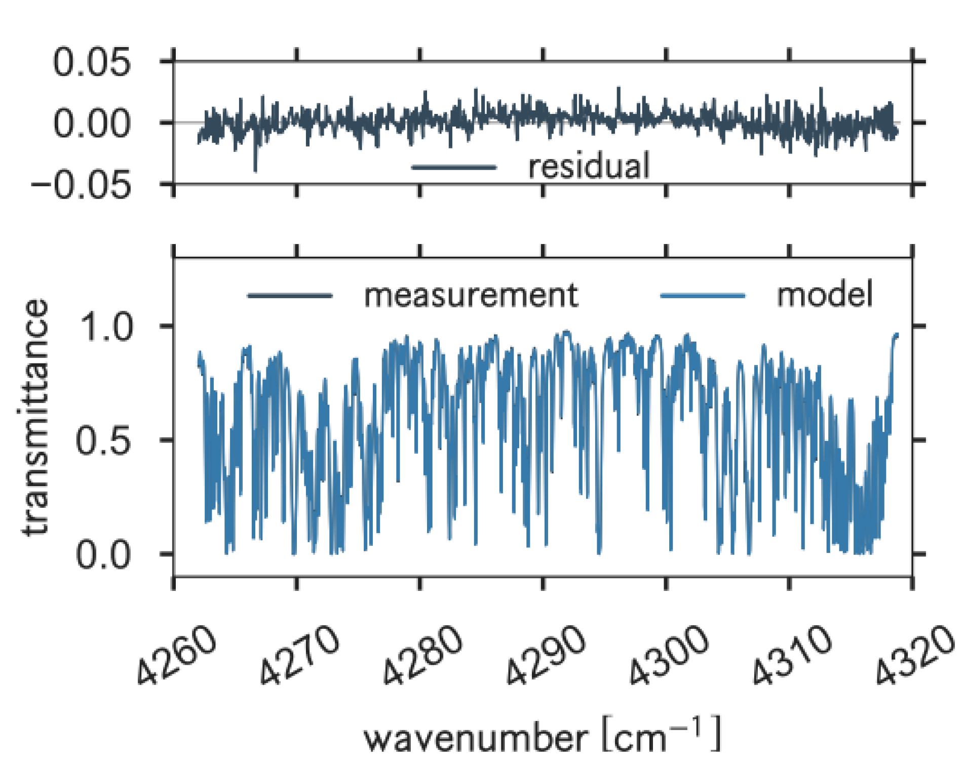
| CO | 4208.7–4318.8 | CH4, H2O, HDO |
| O2 | 7765.0–8005.0 | H2O, HF, CO2 |
| ΔXH2O | ΔXCO2 | ΔXCH4 | ΔXCO | |
|---|---|---|---|---|
| ΔME = 1% | 0.0492% | 0.1151% | 0.1042% | 0.0523% |
| ΔME = −1% | 0.0368% | 0.1707% | 0.0863% | 0.0452% |
| ΔPE = 0.01 | 0.697% | 0.689% | 0.652% | 0.737% |
| ΔPE = −0.01 | 0.715% | 0.729% | 0.689% | 0.775% |
| Distance/cm | ME | PE |
|---|---|---|
| 401 | 0.9572 | 0.00569 |
| 519 | 0.9658 | 0.00613 |
| 605 | 0.9602 | 0.00598 |
| mean | 0.9611 | 0.00593 |
| Standard deviation | 0.00437 | 2.23681 × 10⁻⁴ |
| Distance/cm | ME | PE |
|---|---|---|
| 396 | 0.9591 | 0.00504 |
| 496 | 0.9622 | 0.0048 |
| 596 | 0.963 | 0.00508 |
| 696 | 0.9657 | 0.00571 |
| mean | 0.9625 | 0.00516 |
| Standard deviation | 0.00272 | 3.89081 × 10⁻⁴ |
Publisher’s Note: MDPI stays neutral with regard to jurisdictional claims in published maps and institutional affiliations. |
© 2021 by the authors. Licensee MDPI, Basel, Switzerland. This article is an open access article distributed under the terms and conditions of the Creative Commons Attribution (CC BY) license (https://creativecommons.org/licenses/by/4.0/).
Share and Cite
Liu, D.; Huang, Y.; Cao, Z.; Lu, X.; Liu, X. The Influence of Instrumental Line Shape Degradation on Gas Retrievals and Observation of Greenhouse Gases in Maoming, China. Atmosphere 2021, 12, 863. https://doi.org/10.3390/atmos12070863
Liu D, Huang Y, Cao Z, Lu X, Liu X. The Influence of Instrumental Line Shape Degradation on Gas Retrievals and Observation of Greenhouse Gases in Maoming, China. Atmosphere. 2021; 12(7):863. https://doi.org/10.3390/atmos12070863
Chicago/Turabian StyleLiu, Dandan, Yinbo Huang, Zhensong Cao, Xingji Lu, and Xiangyuan Liu. 2021. "The Influence of Instrumental Line Shape Degradation on Gas Retrievals and Observation of Greenhouse Gases in Maoming, China" Atmosphere 12, no. 7: 863. https://doi.org/10.3390/atmos12070863
APA StyleLiu, D., Huang, Y., Cao, Z., Lu, X., & Liu, X. (2021). The Influence of Instrumental Line Shape Degradation on Gas Retrievals and Observation of Greenhouse Gases in Maoming, China. Atmosphere, 12(7), 863. https://doi.org/10.3390/atmos12070863