Article

Assessing the Risks of Vessel Icing and Aviation Hazards during Downslope Windstorms in the Russian Arctic

by
Anna A. Shestakova
A.M. Obukhov Institute of Atmospheric Physics of the Russian Academy of Science, 119017 Moscow, Russia
Atmosphere 2021, 12(6), 760; https://doi.org/10.3390/atmos12060760
Submission received: 5 May 2021 / Revised: 7 June 2021 / Accepted: 9 June 2021 / Published: 11 June 2021
(This article belongs to the Special Issue Extreme Weather and Climate Events: Global and Regional Aspects)

Abstract

:
Downslope windstorms are known sources of hazardous weather, such as severe gusty winds, rapid temperature changes, ship icing, strong turbulence and others, posing a great danger to people and infrastructure. This paper investigates the risks of ship icing and aviation hazards (rapid changes in the angle of attack and gust load factor) during downslope windstorms in five regions in the Russian Arctic based on observational data, reanalysis, and mesoscale numerical modeling. The highest frequency of ship icing was found during downslope windstorms downstream from Svalbard and Novaya Zemlya. Icing is rare during Tiksi and Wrangel Island downslope windstorms due to almost permanent sea ice cover during the cold season, while icing is absent during very warm Pevek downslope windstorm even in the ice-free conditions. Conditions for heavy icing are rather frequent (up to 5% of cases in winter) during Novaya Zemlya downslope windstorms and less frequent (up to 0.5% in spring) during Svalbard windstorm. The presence of downslope windstorms in those regions causes an increase in the maximum icing rate by about 2 times. Strong aviation turbulence hazardous for light aircraft is typical for all considered regions with downslope windstorms; it is observed mainly at an altitude of 1 to 4 km above the surface. Hazardous turbulence for jet aircraft like Boeing 737 on its cruising flight levels was found on Svalbard and in Tiksi region in 10–15% of cases during strong downslope windstorms.

1. Introduction

Downslope windstorms are generally induced by mountain wave amplification [1], resulting in strong winds on the foot of the lee slope of the mountain. Local winds “bora” and “foehn” (e.g., [2,3]) are a kind of downslope windstorms. In the Arctic, downslope windstorms are known on Novaya Zemlya archipelago (both at its western and eastern sides) [4,5], in Pevek (Chukotka) [6], as well as on Svalbard [7,8,9], in Tiksi (Yakutia) and on Wrangel Island [10]. A review on satellite observations of these winds is given in [11]. The climatology of these winds is summarized in [12,13]. According to station observations, the strongest downslope windstorms are observed on Novaya Zemlya and in Pevek (with gusts up to 50 m s−1), and the weakest on Svalbard [
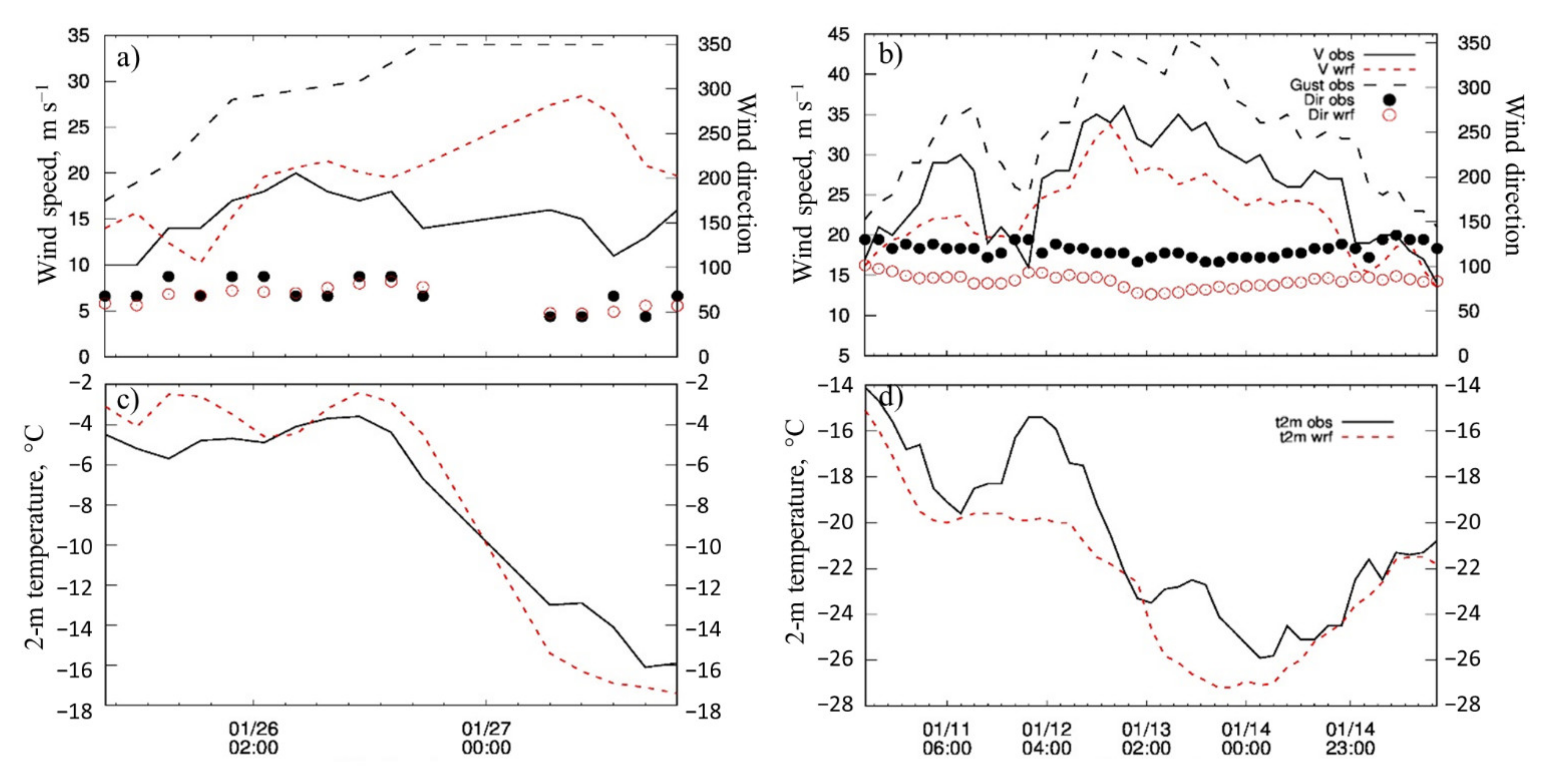
13]. Downslope windstorms on Svalbard and Novaya Zemlya frequently occur with an easterly background flow (Figure 1a,d), although there are also downslope windstorms on the east coasts [4]. Downslope windstorms on Svalbard are usually called “foehns” (e.g., [8,9]), though only half of times they lead to temperature increase (Figure 1b). Downslope windstorms on Novaya Zemlya, called “bora”, are observed very frequently (on average, 138 days per year). In 4% of cases its speed exceeds 30 m s−1. This downslope windstorm could lead to both increase and decrease in air temperature (Figure 1e). In Tiksi and Pevek, downslope windstorms occur about 80 days per year with southwesterly and southeasterly winds, respectively, therefore, they are usually accompanied by a sharp increase in temperature (Figure 1h,k), especially in Pevek. On Wrangel Island downslope windstorm is recorded at a meteorological station with a northerly air flow, with a nearly equal probability of temperature increase and decrease during downslope windstorm (Figure 1n). This wind is rather mild but occur frequently (on average, 95 days per year). Incoming flow in the troposphere for all downslope windstorms usually consists of three layers with different temperature stratification: lowest near-neutral or even unstable layer, an elevated inversion (less pronounced on Svalbard) and a layer with a lapse rate of standard atmosphere above (Figure 1c,f,i,l,o).These downslope windstorms have not previously been considered in detail in terms of the accompanying weather hazards for transport, such as vessel icing and turbulence causing aviation hazards.
Severe turbulence encountered by aircraft was observed many times during downslope windstorms [14,15,16,17,18]. For instance, Ralph et al. (1997) analyzed the case of strong turbulence near the tropopause due to mountain waves that were observed simultaneously with the Chinook downslope windstorm on the eastern slopes of the Rocky Mountains; as a result, the engine and part of the wing were torn off one of the aircraft. Such turbulence occurs due to internal gravity waves that propagate upward from the mountains when the air flows over an obstacle. These waves, under favorable conditions, amplify and break, creating local unstable layers with enhanced turbulence. However, even in the absence of wave breaking, these waves induce strong vertical motions that pose a danger to aviation. Also, strong turbulence could occur on the lower layers, due to lee waves and hydraulic jumps. The latter occurs when flow transits from supercritical to subcritical state at some distance from the lee slope or just over the slope. Hydraulic jumps are often observed during severe downslope windstorms [19]. Most of research considers hazardous turbulence in the upper troposphere, on flight legs of commercial jets.
To assess the risk of aviation hazards, the use of reanalysis is not convenient, since their resolution is not enough to accurately reproduce orography that creates high-amplitude gravity waves. The author is not aware of observational data on such turbulence in the Arctic. Therefore, the only possible tool for assessing aviation hazards during downslope windstorms is numerical model with high spatial and vertical resolution. It is very costly to estimate the frequency of turbulence occurrence with high-resolution model in every considered region since long-period calculations require too many computational resources and time. In this paper, estimations of the characteristic intensity, regions of occurrence and the height where aviation turbulence arise in each region are presented for several cases of strong downslope windstorms.
Many predictors can be used to assess potential areas of clear air turbulence (including orography-induced). For instance, the Graphical Turbulence Guidance System [20] includes many such predictors: Richardson number, frontogenesis function, eddy dissipation rate and others. In this research, the emphasis is not on the calculation of atmospheric turbulence characteristics, but on the calculation of characteristics that directly assess the danger to aircraft associated with strong vertical motions. International Civil Aviation Organization (ICAO) has adopted special indicators for wind shear: F-factor and I-factor [21]. However, these indicators can only be calculated for a specific flight tracks (e.g., [17,22]), since they include the wind speed along the flight track. In the general case, to assess the potential of hazardous aviation turbulence for the region as a whole, the headwind speed is unknown (since the flight route can be any). Indicators that are depend only on vertical velocity and aircraft technical features are used here. These indicators are aircraft angle of attack change and load factor change, which were proposed as predictors of aviation turbulence (this definition is used throughout the paper) in the classic monograph on aircraft aerodynamics [23] and were used in a number of Russian studies devoted to the safety of flights over mountains of Iran, Crimea, Adygea, Kuznetsk Alatau (Siberia), Dzhugdzhur Mountains (Russian Far East), and Karatau Mountains (Kazakhstan) on the basis of simulations [24,25,26].
Vessel icing is one of the greatest hazards to shipping in the Arctic [10,27,28]. Most often, vessel icing occurs when splashing seawater by sea waves [29,30]. This type of icing is called spray icing. During downslope windstorms, the wind speed increases significantly and the temperature sometimes decreases sharply on the lee side of the mountains (Figure 1b,e,h,k,n) when cold air advection, which creates the preconditions for the occurrence of spray icing. Such downslope windstorms create three-dimensional steep sea waves [31] that in company with strong gusty wind ripping off droplets form the wave crests provide the source of spray. For instance, ship icing is frequently observed during Novorossiysk bora (Russian coast of Black Sea), causing great damages [32,33]. According to Russian Barents Sea Pilot [29], icing is especially intense in the coastal waters of the Novaya Zemlya archipelago. Panov (1978) mentioned that icing in the Barents Sea is most frequently observed during the northeasterly winds. Thus, one may suggest the influence of bora on this local icing maximum. Indeed, Bryazgin and Dementiev (1996) mentioned the fact of vessel icing during Novaya Zemlya bora. Recently (28 December 2020) the ship Onega sank in the Barents Sea, 17 people died (https://www.bbc.com/news/world-europe-55467244 (accessed on 9 June 2021)); rapid ice accretion is called one of the versions of this accident. This happened during the Novaya Zemlya bora with wind gusts up to 32 m s−1. Vessel icing was also observed during downslope windstorms in Svalbard [27], despite the frequently occurring temperature rise (see Figure 1b and [13]), which should reduce possible icing.
Ship observations of icing are clearly not enough to assess the risk of vessel icing in the Arctic. There are many methods for estimating the icing rate, most of which are based on the heat balance of the ship surface, on which the sprayed water freezes (e.g., [34,35,36,37]). This approach shows satisfactory results when compared with observational data [34,38] and allows calculations on the basis of reanalysis, since the input parameters (wind speed, air and sea surface temperature, air humidity, radiative fluxes) are available in all reanalyses. Reanalysis data are widely used for calculating vessel icing and compiling its climatology (e.g., [28,39]).
This research aims to obtain an assessment of the risks of vessel icing and aviation turbulence during downslope windstorms in five regions in the Arctic: on the western coasts of Svalbard and Novaya Zemlya, in Tiksi and Pevek, and on Wrangel Island (see Figure 1 and Figure 2). Section 2 describes the methods used to calculate vessel icing and aviation turbulence, the observational data involved, and a description of the numerical simulations. Section 3 and Section 4 present the results of the risks assessment. The main findings are summarized in Section 5.

2. Materials and Methods

2.1. Study Areas and Observational Data

Figure 2 shows the study areas of downslope windstorms on Svalbard and Novaya Zemlya, in Tiksi and Pevek, and on Wrangel Island. Among all the regions, the highest mountains are on Svalbard (up to 1713 m). On Novaya Zemlya archipelago the orography height gradually increases from south to north (in the north the mountains are covered with glaciers and the orography is not as rugged as in the center and in the south). The maximum height of Novaya Zemlya mountains is 1547 m. In Tiksi region, a downslope windstorm occurs when air flows over the Verkhoyanskiy and Kharaulakhskiy ridges with a height of up to 700 m. The Pevek ridge is small (about 6 km wide and 14 km long) and low (up to 616 m). On Wrangel Island mountains stretch from west to east and reach 1096 m.
Figure 1 and Figure 2 also show the location of the weather stations in these areas. The largest coverage by meteorological stations is on Svalbard (figures show only those stations that are used here); in other regions only one meteorological station in every region is operating at the moment. At Russian meteorological stations, measurements are taken eight times a day, at Norwegian ones (which are mostly automatic)—from 8 to 24 times a day. Wind speed measurements at these stations were used to verify the simulation results (see Appendix A). Here, the same criteria for identifying downslope windstorms were used as in [13]: a specific wind direction for each region, a wind speed of more than 8 m s−1, and a duration of more than 6 h.
Ship observations, collected in the ICOADS3 database (International Comprehensive Ocean-Atmosphere Data Set Release 3) [40], were used to study the cases of vessel icing. This database includes the following observations of icing: its type (mechanism), intensity (in gradations: no freezing, slow freezing, fast freezing, slow melting and fast melting of ice) and the ice thickness. Observations in the Russian Arctic (north of 67° N) for the period 1966–2019 were considered in this work.

2.2. Estimation of Vessel Icing

Icing rate dh/dt was calculated on the basis of reanalysis data (see Section 2.4) to assess the risk of vessel icing during downslope windstorms. A modified Overland method [37] (“Overland bulk 2” in [38]), was chosen for this task. This method is based on heat balance between heat releases from freezing water Q f , heat flux from spray Q d , turbulent sensible Q c and latent Q e heat fluxes from the atmosphere, and radiative flux Q r
Q f = Q d + Q c + Q e + Q r
where Q f = L f s ρ i d h d t , Q d = C w R w T f T s . L f s is the latent heat of fusion, C w is the specific heat capacity of water, ρ i is the ice density (890 kg m−3), T f is the seawater freezing temperature (−1.8 °C), T s is the sea surface temperature.
Spray occurs due to collision of the vessel with sea waves or by the wind blowing off droplets from the wave crests. The spray is then transported onto the ship by the wind. The resulting spray flux R w can be expressed in terms of the icing rate using the ratio of freezing water n
R w = ρ i n d h d t
Then from Equation (1) the following expression for the icing rate is obtained by
d h d t = Q r + Q c + Q e ρ i L f s C w n T f T s
where h is the ice thickness., n was taken as 0.5 following [38]. Heat fluxes are calculated using bulk formulas:
Q c = ρ a C p C H U T f T a
Q e = ρ a L e C E U q f q a
where ρ a is the air density, C p is specific heat capacity of air, L e is the latent heat of vaporization, U is wind speed, q f is specific humidity at the freezing temperature, T a and q a are air temperature and specific humidity, respectively. Wind speed, air temperature and humidity were taken at 10-m AMSL. C H and C E are bulk-transfer coefficient for heat and moisture, respectively. In our case, stratification was taken into account using stability functions from [41], and the roughness coefficient was calculated using Charnock’s formula. A more detailed description of the method can be found in [16]. The “Overland bulk 2” method gives fairly good results when compared with ship observations, does not overestimate the bulk-transfer coefficient as much as the original version of this method, and is relatively simple compared, for example, to the complex Marine-Icing model for the Norwegian Coast Guard [42]. Icing is considered light when dh/dt is less than 0.7 cm h−1, moderate when dh/dt is 0.7–2 cm h−1, and severe (or heavy) at an icing rate of more than 2 cm h−1 following [37].

2.3. Estimation of Aviation Turbulence

In this paper, aviation turbulence induced by downslope windstorms and associated gravity waves was estimated with two indicators: a change in the angle of attack Δα and a gust load factor Δn [23,24,25,26]. These indicators were calculated as
Δ α = tan 1 w V
Δ n = q ρ V w
where w is the vertical velocity, V is the airplane speed, ρ is the air density, q is an empirical coefficient, depending on the aircraft characteristics
q = K w C y α S 2 m g
S is wing area, m is aircraft weight, g is acceleration of gravity. Kw is a gust alleviation factor varying from 0.6 to 0.95 [23,43]. C y α is derivative of the lift coefficient with respect to the angle of attack (a so-called lift curve slope) and is an important aerodynamic characteristic of the wing.
Δα shows hazards associated with a rapid change in the angle of attack of an aircraft wing. If the angle of attack exceeds a certain limit, then aircraft stall occurs. Generally, the angle of attack, which is a sum of horizontal flight angle of attack α h f and Δα, should not exceed 9° [24]. Since α h f usually varies from 1° to 7°, then the critical value for Δα varies from 2° to 8°. In this paper, a value of Δα greater than 6° is considered dangerous, following [25]. The second indicator Δn shows changes in the load factor of the aircraft (through changes in the angle of attack and lift of the wing), induced by vertical air motions. The buffeting, caused by gust loads, is moderate when Δn > 0.2, strong when Δn > 0.5 and severe when Δn > 1 [23]. Here, the critical value for Δn was taken as 0.2, following [24,25].
Aircraft characteristics vary greatly even within the same aircraft class. Therefore, the aviation hazards indicators were calculated for two specific aircraft belonging to different classes: (i) piston-engine lightweight aircraft and (ii) jet-engine and medium-weight (according to the ICAO wake turbulence category) aircraft. The most popular models all over the world in each class were chosen, namely Cessna 172 (hereafter, C172) and Boeing 737–800 (hereafter, B737), respectively. Table 1 shows aircraft characteristics that were used for the calculations (see https://cessna.txtav.com/en/piston/cessna-skyhawk#_model-avionics and https://en.wikipedia.org/wiki/Boeing_737_Next_Generation websites (accessed on 9 June 2021)). The maximum take-off weight was taken for m, though the real weight varies during the flight. C y α was taken off the lift coefficient vs angle of attack graph found on http://airfoiltools.com/airfoil/details?airfoil=b737b-il (accessed on 9 June 2021) for B737 and in [44] for C172. Kw depends on aircraft weight and wing parameters; it was calculated according to formula (16–45) in [43]. All the aforementioned discussion on aviation hazards indicators is true only for the level steady flight without maneuvers. Hazards due to vertical wind gusts increases significantly in the take-off and landing flight phases. Thus, here only aviation hazards during the cruise phase is considered. For that reason, Δn and Δα were calculated only at those altitudes at which flight legs usually pass during the stage of level flight. V in the Table 1 is cruise speed.
The main variable parameter in the formulas (2) and (3) is the vertical velocity, which can reach large values during downslope windstorms (e.g., [45]). Adequate simulation of vertical velocity over the mountains requires a high model resolution (with a grid spacing that allows accurate reproduction of orography). The indicators of aviation turbulence were calculated on the basis of simulations of several episodes of strong downslope windstorms in each region with a horizontal resolution of 0.6–1 km (see Section 2.5). At each time period, for each grid cell, the maximum value of Δα and Δn in a column (at altitudes from 1 to 5 km AMSL for C172 and from 9 to 12 km AMSL for B737) was found and assigned to this cell. Then, the maximum value of Δα and Δn, the frequency of hazardous aviation turbulence (the percentage of times when at least one of the parameters exceeded the critical value) and the average height of hazardous aviation turbulence were found for each grid cell using simulations of all episodes. The average height of hazardous aviation turbulence is thus means the average height of its center, though hazardous turbulence can also be observed above/below this height.

2.4. ASR v2

Icing rate was calculated with formula (1) on the basis of Arctic System Reanalysis version 2 (ASR v2) with spatial resolution of 15 km, with temporal resolution of 3 h and temporal coverage from 2000 to 2016 (https://doi.org/10.5065/D6X9291B (accessed on 9 June 2021)). For each region, all reanalysis times were selected that coincided with the downslope windstorms calendar, compiled earlier based on observations at weather stations Ny-Alesund, Malye Karmakuly, Tiksi, Pevek, and Wrangel Island [13]. Although the resolution of the reanalysis is insufficient for accurate reproduction of the spatial structure of downslope windstorms, however, the wind speed enhancement during downslope windstorms is reproduced by reanalysis in the overwhelming majority of cases in all studied regions except Pevek, where only 49% of cases are reproduced (due to the very small size of the Pevek ridge) [46]. For all stations except Pevek, the mean model bias does not exceed 2.5 m s−1 in wind speed and 6 degrees in wind direction; the correlation coefficient between observations and reanalysis is everywhere equal or higher than 0.8 [46]. Thus, one must be careful with the icing rate statistics obtained in this paper for Pevek region, while the estimates obtained for other regions are more reliable.

2.5. Numerical Simulations

Numerical simulations with the WRF-ARW v4.2 model with a high spatial resolution were performed for 25 episodes (5 in each region) of strong downslope windstorms with maximum observed wind speeds up to 40 m s−1 (see Appendix A). Aviation turbulence as well as the vessel icing rate were calculated for these episodes on the basis of model outputs.
Nested domains were used to achieve high resolution (Figure 2). The resolution of the innermost domain was 1 km (600 m in Pevek region). Two domains with a horizontal resolution of 5 km in the outer domain and 1 km in the inner domain were used for Svalbard and Novaya Zemlya regions. In other regions, three domains were used, with the horizontal resolution of 15 km, 3 km, and 1 km (600 m in Pevek region), respectively. Resolution in Pevek region was increased because of very small size of Pevek mountain ridge. Vertical grid spacing monotonically increases from 50 m in the lowest layer to 430 m at 2.5 km height and remains constant (about 480 m) higher. Height of the lowest level is about 20 m; the total number of levels is 50. The ERA5 reanalysis [47] was used as the initial and boundary conditions; it was chosen due to its relatively high resolution (about 30 km) and large temporal coverage.
Additionally, two cases of downslope windstorms (10–15 January 2006 on Novaya Zemlya and 25–27 January 2015 on Svalbard) were simulated with flat terrain (orography height was everywhere set to zero). All other parameters of the experiments were set the same as for the control experiments. These additional experiments called “Flat” were performed to determine the role of downslope windstorms in the vessel icing by comparing “Flat” experiments, where there were no downslope windstorms, with the control ones.

3. Frequency and Intensity of Vessel Icing during Downslope Windstorms

Figure 3a shows all cases of vessel icing for the period 1966–2019 in the Russian Arctic, found in the ICOADS3 database. Comparison of these data and downslope windstorms calendars in different regions revealed several cases of icing (Figure 3b,c) during downslope windstorms on Svalbard and Novaya Zemlya (the absolute majority of them are spray icing). In all these cases, slow freezing, slow melting or no freezing (meaning that icing occurred before the observation period) was observed. The ice thickness was in most cases 1–2 cm, but in two cases it reached 6 cm (24 January 1996 in Svalbard region and 8 February 2001 in Novaya Zemlya region). In the rest of the regions, no cases of icing during downslope windstorms were detected, possibly not only because of the low intensity of icing in these regions, but also because of the small number of observations in the eastern Arctic and ice cover during the cold period, when most of strong downslope windstorms are usually observed [13].
Figure 4 shows calculated icing rate on the basis of reanalysis data for some cases of observed icing. In general, the chosen method reproduces icing in the area where it was observed. However, there are several cases when a point with icing observations falls on an area with sea ice in the reanalysis (for example, at 18:00 26 November 2012 and at 06:00 5 April 2006, Figure 4). The observations themselves do not provide accurate information on where the icing was observed, since it could have occurred before the time of observation, and the vessel could have deliberately moved into the sea ice to reduce icing (a standard method for dealing with vessel icing [34]).
Statistics on the icing rate, calculated on the basis of reanalysis data for the period 2000–2016, is consistent with the observations: the highest among all considered downslope windstorms frequency of vessel icing is noted for the Novaya Zemlya and Svalbard downslope windstorms (Table 2). The intensity of icing is light in the overwhelming majority of cases, and the proportion of cases with moderate icing (of the total number of times when downslope windstorm was observed) reaches 15% in Svalbard region and 26% in Novaya Zemlya region (Figure 5, Table 2). The maximum frequency of heavy icing reach 0.2% in Svalbard (in winter and spring) and 2% in Novaya Zemlya (mainly in winter) regions. According to these calculations, the icing rate during the Novaya Zemlya downslope windstorms reach 7 cm h−1, which is a very heavy icing. In Tiksi and Pevek, icing is practically not observed, but on the contrary, conditions for ice melting prevail (the mean value of icing rate is negative). On Wrangel Island, bora is accompanied by light icing in 30–50% of cases, and by moderate icing in 1–4% of cases.
Figure 5a shows that the predominant icing area in Svalbard region is the northern tip of the archipelago, close to the sea ice edge position. This is due to cold air outbreaks onto the open sea surface in the Fram Strait usually observed along with downslope windstorm. Also tip jets are usually observed to the south and to the north of Svalbard (e.g., [48]), which are favorable for icing due to increased wind thereof. The percentage of cases with moderate to heavy icing directly off the western shores of the archipelago, in the areas of direct downslope windstorm influence, is rather small (Figure 5c). The highest frequency of heavy icing is in the fjords and off the coast of southern Spitsbergen. The picture is different on Novaya Zemlya: the area of the highest frequency of moderate (and also heavy) icing is extended along the western coast and is maximal near the coast (Figure 5b,d). In winter and spring, heavy icing was found along the entire coast (although in spring no icing is observed in the very north due to sea ice) with a maximum in the north in winter and in the center of the coast in spring.
It may seem that much of the icing cases on Novaya Zemlya and Svalbard are related to cold air outbreaks that are observed simultaneously with downslope windstorms. However, the effect of downslope windstorms itself on the vessel icing can be revealed when analyzing simulations with and without orography (Figure 6). Areas of maximum icing rates in the control experiment (Figure 6b,e) coincide with areas of strong downslope wind near the coast; the icing rate decreases sharply in wakes (for example, downstream the Northern Spitsbergen). In the control experiments, as well as in the calculations with reanalysis (Figure 6a,d), vessel icing reaches the degree of heavy icing, which does not occur in the “Flat” experiments (Figure 6c,f). The maximum icing rate in the experiment with (without) the influence of downslope windstorms is 3.2 (1.7) cm h−1 in the Novaya Zemlya region and 2.6 (1.1) cm h−1 in Svalbard region. Thus, downslope windstorms in these regions approximately double the maximum icing rate. In the absence of orography, the area occupied by moderate icing increases in comparison with the control experiment, while the area of light icing decreases in the “Flat” experiments. This is due to the spatial structure of the wind pattern characteristic of downslope windstorms, namely jets and wakes, which are absent in the experiment without orography.
Figure 7 explains the reasons for the change in the icing rate under the influence of downslope windstorms. Three regions can be distinguished where the effect of downslope windstorms on the near-surface wind speed, temperature and humidity was different. On Novaya Zemlya, specific humidity and temperature increased everywhere on the mountains lee side (due to partial blocking of colder and drier air by mountains) in the “WRF” experiment comparing with “WRF Flat” experiment, and at the same time the wind speed increased. Since the air temperature in both episodes was significantly lower than the freezing point of seawater, an increase in temperature and humidity led to a decrease in gradients in formulas (4) and (5), which should lead to a decrease in turbulent fluxes. However, since the effect of the downslope windstorm on the wind speed was much stronger than on the temperature and humidity, the resulting turbulent fluxes increased, which led to increased icing according to (3)–(5). In the northwestern Svalbard, temperature and humidity have also increased due to downslope windstorm, but the wind speed decreased due to wake formation. All three of these factors led to a decrease in icing rate (Figure 6e,f). Finally, in the south of Spitsbergen, a downslope windstorm led to a decrease in air temperature and humidity to the lee of mountains, and the wind speed increased significantly, which led to an increase in icing rate. A decrease in temperature, unusual for foehn winds, occurred in this area due to change in the direction of the incoming flow (compare the direction of the wind on the windward side in Figure 6e,f). The presence of topography forced the air to flow around the archipelago, so the wind direction upwind the southern Svalbard became more northerly, which means that colder air was advected. Thus, the direction of temperature advection had an even greater effect on the resulting temperature on the lee side than the foehn effect (adiabatic heating of the descending air). Summarizing, the wind plays the primary role in the intensification of icing on Novaya Zemlya and in the south of Svalbard during downslope windstorms in considered episodes.
Figure 6 also demonstrates the adequacy of the icing rate calculations with reanalysis, since even at a relatively low resolution compared to simulations, it closely reproduces the icing rate and the main regions with the maximums of this value. The main differences between simulations and reanalysis for the cases shown in Figure 6, as well as for all other cases, are due to differences in the sea ice boundary.
Sea ice cover is the main reason of absence of vessel icing during downslope windstorms in Tiksi and on Wrangel Island. All previous calculations were carried out only for those cells where there is no ice at all (cells with open water). The icing rate for all simulated episodes was also calculated without taking into account the sea ice (not shown), that is, sea ice was replaced by open water in all grid cells, setting surface temperature to 0 °C. Although even the most severe scenarios of global warming do not predict the freeing of the Eastern Russian Arctic from the sea ice by the end of the 21 century in winter and spring (see https://cds.climate.copernicus.eu/cdsapp#!/software/app-globalshipping-arctic-sea-ice-extent-projections?tab=overview (accessed on 9 June 2021)), but some areas are predicted to be ice-free in the autumn. Calculations without sea ice showed that heavy icing occurred in all episodes of downslope windstorms on Wrangel Island, and in four episodes out of five in Tiksi (only moderate icing was observed in one episode). There was no heavy icing even without ice in any of the episodes of Pevek downslope windstorm, where downslope winds bring the strongest warming on the lee side among other regions (Figure 1k, see also [13]). Moderate icing was noted in three episodes of Pevek downslope windstorm, and in the other two, conditions for light icing or ice melting prevailed.

4. Intensity, Characteristic Regions, and Height of Aviation Turbulence during Downslope Windstorms

Simulations revealed the presence of a hazardous aviation turbulence during downslope windstorms in all considered regions for C172 and on Svalbard and in Tiksi region for B737. Figure 8 and Figure 9 shows the maximum values of Δn for each region (a composite of all simulated episodes) for B737 and C172, respectively, Figure 10 shows the frequency of hazardous aviation turbulence for C172, and Figure 11, the average height of hazardous turbulence for C172.
Generally, the highest values of Δn were observed in the valleys downstream from the leeward slopes, while the highest frequency of hazardous aviation turbulence was found on the lee slopes. This is due to the fact that intense downward air motions are always observed precisely over the leeward slope, which causes them. However, upward movements—observed in hydraulic jumps or in lee waves downstream—are usually more intense. The distance from the lee slope at which a hydraulic jump or lee wave is observed can vary greatly, since it depends on the parameters of the incoming flow.
On Svalbard, hazardous aviation turbulence for B737 was found in 11% of all considered cases with downslope windstorms. Though it did not reach the degree of strong. It was found in the north, in Wijdefjorden and in some other areas, as well as in the central part, south of Longyearbyen (Figure 8a), at an altitude of 9–9.5 km. Hazardous turbulence for C172 most often (almost always) was observed over the lee slope of the highest ridge of Spitsbergen, in the northeastern part, and in many other areas, including the Longyearbyen area (Figure 9a and Figure 10a). The typical average height of this turbulence is 2–3 km (Figure 11a).
On Novaya Zemlya, the greatest frequency of hazardous turbulence for C172 was found in the central part of the archipelago (over some slopes, in up to 100% cases), where the orography is very rugged. In the south, in the weather station area, and in the north, this turbulence is less frequent (Figure 10b). The height of this turbulence generally varies from 1 to 3 km (Figure 11b). One of the strongest aviation turbulence was noted in the north, in an intense hydraulic jump on 14–15 January 2006 (Figure 12a). Strong stratification (with the Brunt-Väisälä frequency of 0.03 s−1) and mild wind speed (on average, from 4 to 8 m s−1) in the incoming flow contributed to low Froude number. A nonlinear flow regime with a hydraulic jump (according to the hydraulic theory) or a zone of low-level wave breaking (according to wave theory) forms in such a case [19]. For the example in Figure 12b, vertical velocity in a hydraulic jump reached 10 m s−1.
In Tiksi region, hazardous turbulence for B737 (Figure 8b) was found in 14% of all cases with a downslope windstorm. It occurred when gravity waves propagated to the stratosphere and just under the tropopause they amplified due to a decrease in air density and possibly resonance effects (Figure 12c,d). The vertical velocity at altitude of 10 km reached 6 m s−1 (Figure 12d). Hazardous turbulence for C172 was most often observed on the lee slopes of the Verkhoyanskiy and Kharaulakhskiy ridges (almost in all cases) (Figure 10c), but the strongest turbulence was at their foot, in the valleys (Figure 9c). This area of strong turbulence in the valley between Verkhoyanskiy and Kharaulakhskiy ridges was quite stationary; it might shift slightly, but was observed in all simulated episodes.
In the Pevek region, hazardous turbulence for C172 was noted not only in Pevek itself, but also over other ridges to the east (Figure 9d). The frequency of this turbulence over the Pevek ridge and ridges to the east reached 100% (Figure 10d). The height of the turbulence varied widely, from 1 to 5 km, but in areas with the maximum frequency, it was usually 1–2 km (Figure 11d).
There was a moderate aviation turbulence for C172 above the Wrangel Island weather station and a strong turbulence in the mountains to the west (Figure 9e). Above the highest mountains and their lee slopes, this turbulence was almost always present according to simulations (Figure 10e). The average height of this turbulence was 1.5 km (Figure 11e).

5. Conclusions

Five regions with downslope windstorms in the Russian Arctic were considered for the risk assessment of hazardous vessel icing and aviation turbulence. Chosen methods of calculating the icing rate and aviation turbulence parameters were applied to reanalysis and/or simulations. The latter were performed for severe episodes of downslope windstorms with the WRF-ARW model with high spatial resolution. The following results were obtained.
The highest frequency of hazardous vessel icing was noted for Novaya Zemlya and, to a lesser extent, for Svalbard downslope windstorm. The low frequency of icing on Wrangel Island and in the Tiksi region is associated primarily with sea ice cover most of the year, since in the absence of ice, as idealized calculations on the basis of simulations for strong episodes have shown, the icing was heavy in the vast majority of simulated episodes. Thus, if cold-season sea ice in the Eastern Russian Arctic ever disappear in the future, one could expect heavy icing during strong downslope windstorms in these regions. Even the fact that downslope windstorms in Tiksi lead to a temperature rise in most of the cases [13] does not prevent ships from icing, as in Svalbard. On the contrary, icing in Pevek region was light to moderate even in the absence of sea ice and even for strongest downslope windstorm episodes, because this downslope windstorm is very warm.
The highest icing rate was found for Novaya Zemlya downslope windstorm; in some areas near the coast, the frequency of heavy icing can reach 5% of cases. This is explained, firstly, by the very high wind speed during this downslope windstorm and, secondly, by proximity of the western coast of Novaya Zemlya to climatological mean sea ice edge position [49]. Since the downslope windstorm itself does not propagate far into the sea, the areas of heavy icing are concentrated near the coast. Numerical experiments with and without taking into account the orography (and, consequently, the downslope windstorm) for the regions of Novaya Zemlya and Svalbard have shown that it is downslope windstorm that leads to the occurrence of severe icing off the coast. Downslope windstorms lead to an approximate two-fold increase in the maximum icing rate.
Aviation turbulence, hazardous for light aircraft Cessna 172, was found in all considered regions in each of the simulated episodes of strong downslope windstorms. This turbulence occurred very frequently and not only over the mountains, but also downstream, over the sea, due to lee waves and hydraulic jumps. Typical regions where this turbulence occur most frequently in simulations were revealed. In most regions, hazardous turbulence occurred at altitudes from 1 to 4 km. Hazardous turbulence for Boeing 737, calculated at altitudes of cruising flight levels FL300–FL390, was found on Svalbard (in 11 % of cases) and in Tiksi region (in 14 % of cases). The average height of this turbulence is 9–10 km.
The icing rate calculations using the “Overland bulk 2” method [38] give reasonable results. The calculations based on reanalysis data and simulations are close. The main difference in icing rate between these two calculations are due to difference in sea ice extent. Note that the obtained statistics on icing rate is a rather rough estimate and not exact values for several reasons. First, all icing methods, including the one used here, do not take into account a lot of factors—such as the type of the ship, surface orientation, etc.—and the percentage of freezing water is artificially set by a constant. Secondly, there are inaccuracies in meteorological parameters in the reanalysis, especially when considering such a mesoscale phenomenon as downslope windstorm.
Since only five episodes of downslope windstorms were simulated in each region, the obtained results on ship icing and aviation turbulence during strong downslope windstorms are not statistically secured. Another limitation of this work is the choice of indicators for evaluating aviation turbulence. Here only the aviation turbulence caused by intense vertical motions was considered, but hazards from turbulent layers induced by wave breaking, as well as turbulence due to wind shear were not taken into account. Both unaccounted for turbulence undoubtedly should take place during downslope windstorms. Moreover, only during the level flight all the assessment were obtained, while the presence of turbulence during aircraft maneuvers is usually even more dangerous.
Simulations and reanalysis data cannot fully replace observations, however, in the absence of the latter in such remote regions as the Arctic, it is believed that the results obtained can be useful in planning economic activities and transport routes in the Arctic.

Funding

This research was funded by the Russian Foundation for Basic Research, grant no. 18-05-80065.

Data Availability Statement

Arctic System Reanalysis version 2 and ICOADS3 database are available at the National Center for Atmospheric Research (NCAR) Data Archive website (https://rda.ucar.edu/ (accessed on 9 June 2021)). ECMWF ERA5 reanalysis is available via Copernicus Climate Change Service [47].

Acknowledgments

The author acknowledge the NCAR and Copernicus Climate Change Service for making available datasets used in this study. The author also thanks Myslenkov S.A. and Arkhipkin V.S. for providing access on supercomputer where the WRF model was run.

Conflicts of Interest

The author declares no conflict of interest.

Appendix A

Five downslope windstorm episodes in each considered region (Table A1) were selected to perform simulations in order to assess the aviation turbulence and vessel icing during strong downslope windstorms with the wind speed of 20–40 m s−1.
For each of the episodes, the simulation results were compared with observational data at meteorological stations (see examples on Figure A1). Table A2 presents statistical estimates of the model wind speed error averaged over all episodes in each region. In Svalbard, comparison was made for all four stations located in different parts of the archipelago (Figure 1 and Figure 2); Table A2 and Figure A2 show the values averaged over all these stations. On average, the model underestimates the wind speed during downslope windstorms in all regions, especially in Pevek, except for Svalbard, where, on the contrary, a systematic overestimation is noted (Figure A1 and Figure A2). Simulation results for Wrangel Island have the lowest correlation coefficient among other regions, but also the smallest bias. The regions of Novaya Zemlya, Pevek, Tiksi are characterized by a particularly strong wind speed underestimation at high wind speeds (Figure A2a). The mean absolute error in wind speed for all regions except Pevek does not exceed 5 m s−1 (in Pevek it is 5.6 m s−1). In general, the quality of modeling downslope windstorms was considered as satisfactory given the complexity of the simulated phenomenon and high wind speeds.
Table A1. Episodes of strong downslope windstorms in each region chosen for simulation and maximal observed wind speed.
RegionEpisodeMaximal Wind Speed, m/sRegionEpisodeMaximal Wind Speed, m/s
Svalbard28–30 November 200523 Pevek14–16 March 200631
26–28 January 2010256–8 December 200835
25–27 January 20152016–18 March 200933
28–30 December 201624 27–29 January 201034
6–10 January 20202715–17 December 201034
M. Karmakuly1–3 March 198138 Wrangel Island18–19 January 198028
10–15 January 200636 8–12 March 199225
15–18 May 2008402–3 December 199226
9–13 February 200940 27–29 January 200028
16–18 February 20143110–12 February 200428
Tiksi26–27 December 198034
27–28 December 199530
24–26 October 200230
22–26 December 201528
17–23 January 201730
Figure A1. Time series of (a,b) 10-m wind speed (lines) and wind direction (circles) and (c,d) 2-m air temperature according to observations (black) and simulations (red) at stations Akseloya, Svalbard (a,c) (25–27 January 2015) and Malye Karmakuly, Novaya Zemlya (b,d) (10–15 January 2006).
Atmosphere 12 00760 g0a1
Table A2. Mean model wind speed bias, root mean square error (RMSE), correlation coefficient R and the mean observed wind speed for each region.
Bias, m/sRMSE, m/sRMean Observed Wind Speed, m/s
Svalbard2.13.10.7312.3
M.Karmakuly−35.40.8026.5
Tiksi−1.94.90.6318.7
Pevek−5.26.50.8524.9
Wrangel Island−0.95.40.5118.8
Figure A2. Results of verification: (a) Scatter plot of observed and simulated wind speed in each region and (b) Taylor diagram.
Atmosphere 12 00760 g0a2

References

  1. Klemp, J.B.; Durran, D.R. Numerical modelling of bora winds. Meteorol. Atmos. Phys. 1987, 36, 215–227. [Google Scholar] [CrossRef]
  2. Yoshino, M. Local Wind Bora; University of Tokyo Press: Tokyo, Japan, 1976; p. 289. [Google Scholar]
  3. Richner, H.; Hachler, P. Understanding and forecasting Alpine foehn. In Mountain Weather Research and Forecasting; Chow, F.K., De Wekker, S.F.J., Snyder, B.J., Eds.; Springer: Dordrecht, The Netherlands, 2013; pp. 219–260. [Google Scholar]
  4. Efimov, V.V.; Komarovskaya, O.I. The Novaya Zemlya bora: Analysis and numerical modeling. Izv. Atmos. Ocean. Phys. 2018, 54, 73–85. [Google Scholar] [CrossRef]
  5. Moore, G.W.K. The Novaya Zemlya bora and its impact on Barents Sea air-sea interaction. Geophys. Res. Lett. 2013, 40, 3462–3467. [Google Scholar] [CrossRef] [Green Version]
  6. Zimich, P.I. Pevekskyi Yuzhak; Gidrometizdat: Leningrad, Russia, 1991; p. 120. [Google Scholar]
  7. Skeie, P.; Gronas, S. Strongly stratified easterly flows across Spitsbergen. Tellus 2000, 52, 473–486. [Google Scholar] [CrossRef]
  8. Maciejowski, W.; Michniewski, A. Variations in weather on the east and west coasts of South Spitsbergen. Pol. Polar Res. 2007, 28, 123–136. [Google Scholar]
  9. Migała, K.; Nasiołkowski, T.; Pereyma, J. Topoclimatic conditions in the Hornsund area (SW Spitsbergen) during the ablation season 2005. Pol. Polar Res. 2008, 29, 73–91. [Google Scholar]
  10. Pastusiak, T. Northern Sea Route as a Shipping Lane; Springer: New York, NY, USA, 2016; p. 219. [Google Scholar]
  11. Ivanov, A.Y. Local Katabatic Winds of the Russian Federation and Their Observation Using Synthetic Aperture Radar Imagery. Izv. Atmos. Ocean. Phys. 2020, 56, 989–1006. [Google Scholar] [CrossRef]
  12. Bryazgin, N.N.; Dementiev, A.A. Hazardous Meteorological Phenomena in the Russian Arctic; Gidrometeoizdat: Sankt-Petersburg, Russia, 1996; p. 150. [Google Scholar]
  13. Shestakova, A.A.; Toropov, P.A.; Matveeva, T.A. Climatology of extreme downslope windstorms in the Russian Arctic. Weather Clim. Extrem. 2020, 28, 100256. [Google Scholar] [CrossRef]
  14. Lilly, D.K. A severe downslope windstorm and aircraft turbulence event induced by a mountain wave. J. Atmos. Sci. 1978, 35, 59–77. [Google Scholar] [CrossRef] [Green Version]
  15. Lester, P.F.; Bach, R.E., Jr. An extreme clear air turbulence incidence associated with a strong downslope windstorm. In Proceedings of the 24th Aerospace Sciences Meeting, Reno, NV, USA, 6–9 January 1986. [Google Scholar]
  16. Ralph, F.M.; Neiman, P.J.; Levinson, D. Lidar observations of a breaking mountain wave associated with extreme turbulence. Geophys. Res. Lett. 1997, 24, 663–666. [Google Scholar] [CrossRef]
  17. Maruhashi, J.; Serrão, P.; Belo-Pereira, M. Analysis of mountain wave effects on a hard landing incident in Pico aerodrome using the AROME model and airborne observations. Atmosphere 2019, 10, 350. [Google Scholar] [CrossRef] [Green Version]
  18. Parker, T.J.; Lane, T.P. Trapped mountain waves during a light aircraft accident. Aust. Meteorol. Oceanogr. J. 2013, 63, 377–389. [Google Scholar] [CrossRef]
  19. Durran, D.R. Another look at downslope windstorms. Part I: The development of analogs to supercritical flow in an infinitely deep, continuously stratified fluid. J. Atmos. Sci. 1986, 43, 2527–2543. [Google Scholar] [CrossRef]
  20. Sharman, R.; Tebaldi, C.; Wiener, G.; Wolff, J. An integrated approach to mid- and upper-level turbulence forecasting. Weather Forecast. 2006, 21, 268–287. [Google Scholar] [CrossRef]
  21. International Civil Aviation Organization (ICAO). Manual on Low-Level Wind Shear, 1st ed.; International Civil Aviation Organization: Montreal, QC, Canada, 2005; p. 213. [Google Scholar]
  22. Guan, W.L.; Yong, K. Review of aviation accidents caused by wind shear and identification methods. J. Chin. Soc. Mech. Eng. 2002, 23, 99–110. [Google Scholar]
  23. Nikolaev, L.F. Aerodynamics and Dynamics of Transport Aircraft Flight; Transport: Moscow, Russia, 1990; p. 392. [Google Scholar]
  24. Kozhevnikov, V.N.; Pavlenko, A.P. Atmospheric disturbances over mountains and flight safety. Izv. RAN Fiz. Atmos. Okeana 1993, 29, 780–792. [Google Scholar]
  25. Kozhevnikov, V.N.; Memarian, M.K. Orographic disturbances and the problem of flight safety over the mountains of Iran. Probl. Anal. Riska 2006, 3, 346–361. [Google Scholar]
  26. Berzegova, R.B.; Bedanokov, M.K. Atmospheric Perturbations during the Flow around Mountain Groups. Izv. Atmos. Ocean. Phys. 2018, 54, 456–461. [Google Scholar] [CrossRef]
  27. Samuelsen, E.M.; Graversen, R.G. Weather situation during observed ship-icing events off the coast of Northern Norway and the Svalbard archipelago. Weather Clim. Extrem. 2019, 24, 100200. [Google Scholar] [CrossRef]
  28. Naseri, M.; Samuelsen, E.M. Unprecedented vessel-icing climatology based on spray-icing modelling and reanalysis data: A risk-based decision-making input for arctic offshore industries. Atmosphere 2019, 10, 197. [Google Scholar] [CrossRef] [Green Version]
  29. Main Directorate of Navigation and Oceanography of the Ministry of Defense of the Russian Federation. Barents Sea Pilot, Part II, no 1112; GUNiO: Saint Petersburg, Russia, 1995; p. 496. (in Russian) [Google Scholar]
  30. Panov, V.V. Icing of ships. Polar Geogr. 1978, 2, 166–186. [Google Scholar] [CrossRef]
  31. Shestakova, A.A.; Myslenkov, S.A.; Kuznetsova, A.M. Influence of Novaya Zemlya Bora on Sea Waves: Satellite Measurements and Numerical Modeling. Atmosphere 2020, 11, 726. [Google Scholar] [CrossRef]
  32. Shlygin, I. Popular Hydrometeorology and Navigation; Transport: Moscow, Russia, 1987; p. 192. [Google Scholar]
  33. Mikhailov, V.I.; Zorin, V.Y.; Kapochkina, M.B. On the vulnerability of the Russian fleet and high risks for cargo flows through the ports of Anapa, Novorossiysk, Tuapse. ScienceRise 2015, 4, 31–34. (In Russian) [Google Scholar] [CrossRef]
  34. Panov, V.V. Icing of Ships. In Arkticheskii i Antarkticheskii Nauchno-Issledovatel’skii Institut, Trudy 334; Gidrometeoizdat: Leningrad, Russia, 1976; p. 263. [Google Scholar]
  35. Stallabrass, J.R. Trawler Icing—A compilation work done at National Research Council (NRC). In Mechanical Engineering Report MD-56; National Research Council of Canada: Ottawa, Canada, 1980. [Google Scholar]
  36. Wise, J.A.; Comiskey, A.L. Superstructure Icing in Alaskan Waters; NOAA Special Report; Pacific Marine Environmental Laboratory: Seattle, WA, USA, 1980; p. 30. [Google Scholar]
  37. Overland, J.E.; Pease, C.H.; Preisendorfer, R.W.; Comiskey, A.L. Prediction of vessel icing. J. Clim. Appl. Meteorol. 1986, 25, 1793–1806. [Google Scholar] [CrossRef] [Green Version]
  38. Samuelsen, E.M. Ship-icing prediction methods applied in operational weather forecasting. Q. J. R. Meteorol. Soc. 2018, 144, 13–33. [Google Scholar] [CrossRef]
  39. Moore, G.W.K. A climatology of vessel icing for the subpolar North Atlantic Ocean. Int. J. Climatol. 2013, 33, 2495–2507. [Google Scholar] [CrossRef]
  40. Freeman, E.; Woodruff, S.D.; Worley, S.J.; Lubker, S.J.; Kent, E.C.; Angel, W.E.; Berry, D.I.; Brohan, P.; Eastman, R.; Gates, L.; et al. ICOADS Release 3.0: A major update to the historical marine climate record. Int. J. Climatol. 2017, 37, 2211–2232. [Google Scholar] [CrossRef] [Green Version]
  41. Louis, J.F. A parametric model of vertical eddy fluxes in the atmosphere. Bound. Layer Meteorol. 1979, 17, 187–202. [Google Scholar] [CrossRef]
  42. Samuelsen, E.M.; Edvardsen, K.; Graversen, R.G. Modelled and observed sea-spray icing in Arctic-Norwegian waters. Cold Reg. Sci. Technol. 2017, 134, 54–81. [Google Scholar] [CrossRef] [Green Version]
  43. Gudmundsson, S. General Aviation Aircraft Design: Applied Methods and Procedures; Elsevier: New York, NY, USA, 2013; p. 1048. [Google Scholar]
  44. Fernandes, I.; Sapkota, Y.; Mammen, T.; Rasheed, A.; Rebello, C.; Kim, Y.H. Theoretical and Experimental Investigation of Leading Edge Tubercles on the Wing Performance. In Proceedings of the 2013 Aviation Technology, Integration, and Operations Conference, Los Angeles, CA, USA, 12–14 August 2013; p. 4300. [Google Scholar]
  45. Shestakova, A.A.; Toropov, P.A.; Stepanenko, V.M.; Sergeev, D.E.; Repina, I.A. Observations and modelling of downslope windstorm in Novorossiysk. Dyn. Atmos. Ocean. 2018, 83, 83–99. [Google Scholar] [CrossRef]
  46. Shestakova, A.A.; Repina, I.A. Overview of strong winds on the coasts of the Russian Arctic seas. Ecol. Montenegrina 2019, 25, 14–25. [Google Scholar] [CrossRef]
  47. Copernicus Climate Change Service (C3S) (2017): ERA5: Fifth Generation of ECMWF Atmospheric Reanalyses of the Global Climate. Copernicus Climate Change Service Climate Data Store (CDS). Available online: https://cds.climate.copernicus.eu/cdsapp#!/home (accessed on 1 May 2021).
  48. Reeve, M.A.; Kolstad, E.W. The Spitsbergen south cape tip jet. Q. J. R. Meteorol. Soc. 2011, 137, 1739–1748. [Google Scholar] [CrossRef]
  49. Dai, P.; Gao, Y.; Counillon, F.; Wang, Y.; Kimmritz, M.; Langehaug, H.R. Seasonal to decadal predictions of regional Arctic sea ice by assimilating sea surface temperature in the Norwegian Climate Prediction Model. Clim. Dyn. 2020, 54, 3863–3878. [Google Scholar] [CrossRef] [Green Version]
Figure 1. Study areas: wind speed (color) composite maps for 5 episodes of strong downslope windstorms according to simulations (see Section 2.5) (a,d,g,j,m); topography cross-sections with the graphs showing temperature tendency frequency during downslope windstorms according to observations at stations (adopted from [13]) (b,e,h,k,n); mean potential temperature profile (ratio of potential temperature to potential temperature at the lowest level) in the incoming flow in the lowest 3-km layer according to CFSR reanalysis (see details in [13]) (c,f,i,l,o). Weather stations are shown with white points; empty arrows show the direction of the incoming flow.
Atmosphere 12 00760 g001aAtmosphere 12 00760 g001b
Figure 2. Model domains in (a) Svalbard, (b) Novaya Zemlya, (c) Tiksi region, (d) Pevek region, and (e) Wrangel Island. Color shows orography height (in m above mean sea level (AMSL)); weather stations are shown with red circles.
Atmosphere 12 00760 g002
Figure 3. Cases of vessel icing as observed by ships in the Russian Arctic for the period 1966–2019: (a) all cases, (b,c) cases of icing during downslope windstorms on Svalbard (b) and Novaya Zemlya (c). Color shows the type of icing: 1—spray icing; 2—fog icing; 3—simultaneous spray and fog icing; 4—rain icing; 5—simultaneous spray and rain icing.
Atmosphere 12 00760 g003
Figure 4. Examples of calculated icing rate from reanalysis data for the times when ship icing was observed (red asterisks) in Svalbard (top) and Novaya Zemlya (bottom) regions during downslope windstorms. Wind barbs at 10 m above ground level are also shown according to ASR v2.
Atmosphere 12 00760 g004
Figure 5. Frequency of moderate (a,b) and heavy (c,d) vessel icing (in % of the total number of times when downslope windstorms were observed) during downslope windstorms in Ny-Alesund (a,c) and M.Karmakuly (b,d) according to calculations on the basis of reanalysis.
Atmosphere 12 00760 g005
Figure 6. Icing rate (in cm h−1, color) and wind vectors (barbs) during downslope windstorms on Novaya Zemlya at 18:00 UTC 13 January 2006 (top) and on Svalbard at 12:00 UTC 27 January 2015 (bottom) according to calculations on the basis of reanalysis (a,d) and high-resolution simulation in the innermost domain in the control (b,e) and “Flat” (c,f) experiments.
Atmosphere 12 00760 g006
Figure 7. Differences in 2-m specific humidity (a,d), 2-m air temperature (b,e) and 10-m wind speed (c,f) between simulations with and without orography (“WRF” minus “WRF Flat”) on Novaya Zemlya at 18:00 UTC 13 January 2006 (ac) and on Svalbard at 12:00 UTC 27 January 2015 (df).
Atmosphere 12 00760 g007
Figure 8. Maximal value of Δn for B737 according to simulations in (a) Svalbard and (b)Tiksi region. Contours show orography height (every 300 m).
Atmosphere 12 00760 g008
Figure 9. Maximal value of Δn for C172 according to simulations in (a) Svalbard, (b) Novaya Zemlya, (c) Tiksi region, (d) Pevek region, and (e) Wrangel Island. Contours show orography height (every 300 m).
Atmosphere 12 00760 g009
Figure 10. Frequency of hazardous aviation turbulence (Δn > 0.2 and/or Δα > 6°) for C172 according to simulations (in % of all cases) in (a) Svalbard, (b) Novaya Zemlya, (c) Tiksi region, (d) Pevek region, and (e) Wrangel Island. Contours show orography height (every 300 m).
Atmosphere 12 00760 g010
Figure 11. Mean height (in km AMSL) of hazardous aviation turbulence for C172 according to simulations in (a) Svalbard, (b) Novaya Zemlya, (c) Tiksi region, (d) Pevek region, and (e) Wrangel Island. Contours show orography height (every 300 m).
Atmosphere 12 00760 g011
Figure 12. Vertical cross-sections of (a,c) Δn (color), potential temperature (contours, every 2 K) and wind vector and (b,d) horizontal wind speed (color) and vertical velocity (contours, every 2 m s−1) during Novaya Zemlya bora at 23:00 14 January 2006 along line AB (a,b) and during Tiksi downslope windstorm at 18:00 27 December 1995 along line CD (c,d) (see Figure 9b,c for cross-sections locations).
Atmosphere 12 00760 g012
Table 1. Aircraft characteristics.
Aircraftm, kgS, m2 C y α ,   radian 1 Kwq, m s2 kg−1V, m s−1
Cessna 172115716.24.10.72 × 10−364
Boeing 737–80079,0101256.80.84.4 × 10−4236
Table 2. Ship icing statistics according to calculations from reanalysis: spatially and temporally averaged value of icing rate and maximal values of icing rate and icing frequency in the studied areas ever noted. «-» means there were no icing at all.
Mean dh/dt, cm h−1Maximal dh/dt, cm h−1Maximal Frequency of Light Icing, %Maximal Frequency of Medium Icing, %Maximal Frequency of Heavy Icing, %
Svalbard
Winter0.562.6075.0020.000.3
Spring0.303.1050.0025.000.5
Summer−0.200.00---
Autumn0.202.0060.004.00-
Year0.303.1060.0015.000.2
Novaya Zemlya
Winter0.907.3090.0045.005
Spring0.254.0050.0020.002
Summer−0.250.261.50--
Autumn0.293.1065.0012.000.3
Year0.307.3055.0026.002
Tiksi
Winter-----
Spring-----
Summer−0.400.05---
Autumn−0.051.0035.002.00-
Year−0.101.0025.002.00-
Pevek
Winter-----
Spring0.050.10---
Summer−0.300.06---
Autumn−0.010.7020.00--
Year−0.300.705.00--
Wrangel Island
Winter0.590.95100.0025.00-
Spring-----
Summer−0.200.161.80--
Autumn0.211.3058.005.00-
Year0.111.3046.004.30-
Publisher’s Note: MDPI stays neutral with regard to jurisdictional claims in published maps and institutional affiliations.

