Impact of Tropical Cyclones on Inhabited Areas of the SWIO Basin at Present and Future Horizons. Part 2: Modeling Component of the Research Program RENOVRISK-CYCLONE

Abstract

The ReNovRisk-Cyclone program aimed at developing an observation network in the south-west Indian ocean (SWIO) in close synergy with the implementation of numerical tools to model and analyze the impacts of tropical cyclones (TC) in the present and in a context of climate change. This paper addresses the modeling part of the program. First, a unique coupled system to simulate TCs in the SWIO is developed. The ocean–wave–atmosphere coupling is considered along with a coherent coupling between sea surface state, wind field, aerosol, microphysics, and radiation. This coupled system is illustrated through several simulations of TCs: the impact of air–sea flux parameterizations on the evolution of TC Fantala is examined, the full coupling developed during the program is illustrated on TC Idai, and the potential of novel observations like space-borne synthetic aperture radar and sea turtles to validate the atmosphere and ocean models is presented with TC Herold. Secondly, the evolution of cyclonic activity in the SWIO during the second half of the 21st century is assessed. It was addressed both using climate simulation and through the implementation of a pseudo global warming method in the high-resolution coupled modeling platform. Our results suggest that the Mascarene Archipelago should experience an increase of TC related hazards in the medium term.

1. Introduction

Due to the possible devastating combination of extreme winds, torrential precipitation, storm surge, and high waves, tropical cyclones (TC) are a major threat for impacted territories. This is particularly true in the South-West Indian Ocean (SWIO) that represents 10–12% of the global TC activity [1,2] and includes several countries with precarious economies and fragile infrastructures, making them highly vulnerable to cyclonic risks. Madagascar, which ranks among the poorest countries in the world, is regularly affected by TCs. Between 1999 and 2016, 34 systems directly hit Madagascar, 10 of which as a TC at the time of landfall [3]. In March 2004, TC Gafilo—the most intense TC ever observed in the SWIO at this date—made landfall in the north-east of Madagascar, leaving more than 200,000 victims, 400 deaths, and damages estimated at USD 250 million. In 2017, TC Enawo hit almost the same region of Madagascar at the peak of its intensity (maximum wind speed of 57 m s${}^{-1}$). The associated storm surge, high winds and heavy rains led to 81 deaths, 300,000 victims, heavily damaged structures, and severe losses in rice fields (damages estimated at ∼USD 137 million). Mozambique is also frequently hit by tropical depressions with 16 direct hits between 1999 and 2016 [3]. In 2019, TC Idai made landfall in the region of Beira. Wind gusts and torrential rainfall devastated the crops, destroyed more than 29,500 houses, and damaged tens of thousands of others, leading to a major humanitarian crisis. More than 1000 people died and 2.6 million victims were reported. The damages were estimated at USD 2 billion in the impacted region (Mozambique, Malawi, Zimbabwe, Madagascar). Six weeks later, TC Kenneth, after devastating the Comoros archipelago, hit the north of Mozambique, in the region of Pemba, worsening the humanitarian, sanitary, and economic situation of the country. This high exposure to natural disaster adds to the dependence on agriculture and natural resources and leads to severe humanitarian crises, which are most of the time under-reported in the media.

Due to its relatively small size (∼60 km in diameter), La Réunion (21.1${}^{\circ }$ S, 55.5${}^{\circ }$ E) is not frequently directly hit by TCs but is regularly affected by systems passing at a few tens or hundreds of kilometers away. In 2002, the eye of TC Dina passed more than 65 km away from the north-west of the island. However, due to the strong winds, swell, and heavy rain, damages on the crops and infrastructures—in particular roads and electric networks—were estimated at several hundreds of thousands of euros. In 2007, TC Gamède passed at more than 200 km away from the island, but heavy rainfall (reinforced by the steep orography) and high swell (11.7 m recorded on the north-west shore) affected the island during several days. A rainfall rate of 4936 mm was recorded in 96 h at the Cratère Commerson raingauge station [4]. Gamede was at the origin of damages estimated at ∼100 millions of euros. Even if TCs do not directly hit inhabited regions, they can still have considerable economic and sanitary impact.

These few examples show the importance of an accurate forecasting of TC track, intensity, structure, and associated hazards several days in advance to prepare populations and infrastructures, evacuate the most exposed regions, and eventually prepare humanitarian aid. Despite undeniable improvements in TC forecasting, understanding and predicting rapid changes in track, intensity, and structure remain a challenge in particular near landfall [5]. This limitation can be attributed to a lack of observations over the oceans, to models limitations in terms of physical parameterizations and resolution, and to limited understanding of some physical processes involved in TC intensification. To advance in the numerical representation of TCs, it is important to develop coupled models and parameterizations to rely on coherent oceanic and atmospheric fields.

In the context of climate change, improving TC forecasting to protect goods and persons should go along with projections of TC risks on SWIO territories to anticipate and adapt for potential new risks. The impact of global warming on frequency, intensity, and precipitation rates of TCs is thoroughly documented in the literature (e.g., [6,7,8,9,10,11,12]). In a recent study, high-resolution experiments were used to estimate projected changes in cyclonic activity over the South Indian Ocean basin near the end of the century [13]. An interesting result of this study is related to an earlier onset (about 1 month) of the TC season, underlining the need to focus on what is occurring at the regional level.

The ReNovRisk program [14] aims at analyzing risks associated with TCs and their economical impact on the SWIO countries, to improve the resilience capability of those territories facing cyclonic hazards. ReNovRisk-Cyclone (RNR-CYC) is one of the four components of the global ReNovRisk program. It focuses on the meteorological and oceanic impact of TCs on the SWIO countries in the present and in the future. The four components of RNR-CYC and the observations implemented during this program are presented in the companion paper [15]. The objective of this paper is to present the modeling strategy of RNR-CYC in terms of forecasting and climate projection. The outline of the paper is as follows. Section 2 is dedicated to the presentation of the high-resolution modeling platform developed in the framework of this program to improve numerical forecasting of TCs. Several coupled simulations of TCs illustrate these developments in Section 3. Section 4 investigates potential changes in the frequency and intensity of TCs over the period 2015–2094 from high-resolution global climate simulation specifically made in the frame of RNR-CYC. Finally, conclusions and perspectives are given in Section 5.

2. Development of a Coupled System for TC Modeling

One of the main objectives of the RNR-CYC program is to develop and demonstrate the added value of a high-resolution (horizontal grid spacing less than 2.5 km) ocean–wave–atmosphere (OWA) modeling system for forecasting TCs and their impacts. This tool heralds the next generation of operational numerical weather prediction (NWP) systems to be used by Regional Specialized Meteorological Center (RSMC) La Réunion at mid-term.

Since an important source of energy for TCs is the heat and moisture extracted from the underlying upper ocean, the ocean–atmosphere coupling is increasingly considered as essential in numerical modeling of TCs (e.g., [16,17,18,19]). Coupled OWA models (e.g., [19,20,21,22,23]) have started being developed to deal with the significant role of oceanic waves in air–sea exchanges. Waves modify the wind stress which drives the turbulent fluxes, and the turbulent mixing induced by non-breaking waves is essential to improve the cooling effect underneath and then TC forecasting [24]. Moreover, breaking waves generate sea sprays [25] that can impact TC structure and intensity in several ways. These sea sprays can modify the heat and momentum air–sea fluxes [26,27,28] even if the quantification of the sea spray effect on heat and momentum fluxes is still debated [29]. Sea spray particles are also a source of cloud condensation nuclei [30,31,32], which can modify the microphysical structure and latent heat budget of the TC and consequently its structure and intensity [33]. Moreover, cloud-radiative processes in ice clouds are increasingly recognized to play a major role in the development of TCs (e.g., [34,35]) due to their impact on the secondary circulation. Since convective precipitation and cloud microphysics remain one major cause of systematic errors in numerical models across time scales [36], aerosol–microphysics–radiation interactions must be carefully considered in numerical models to improve TC forecasting.

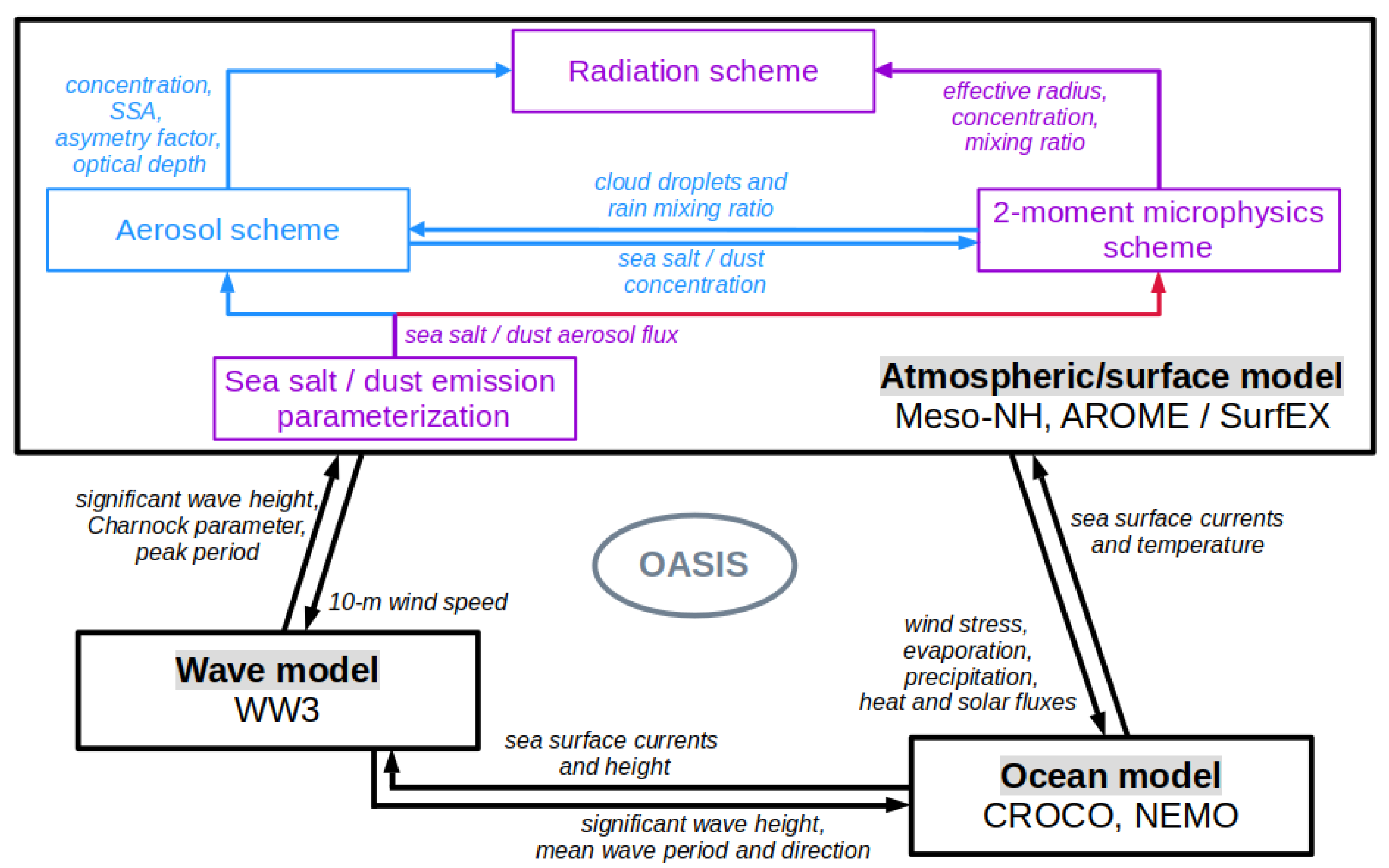
2.1. Ocean–Wave–Atmosphere Coupling

The coupled system presented herein (Figure 1) is based on a combination of state-of-the art numerical models for the atmosphere and the surface, the waves, and the ocean.

2.1.1. Atmospheric Models

For the atmosphere, the Meso-NH research model (http://mesonh.aero.obs-mip.fr/, accessed on 27 May 2021) [37] or the AROME French operational model [38,39] can be used. Meso-NH is the non-hydrostatic mesoscale atmospheric model of the French research community. It incorporates a non-hydrostatic system of equations that enables dealing with a large range of scales (from synoptic to large eddy). It has a complete set of modules and parameterizations for the representation of clouds and precipitation, aerosol, and chemistry but also fires, volcanic eruptions, and atmospheric electricity [37]. Meso-NH is designed to perform both real case simulations and academic cases. It also has a complete set of observation operators to compare model output directly with observations (radar, lidar, GPS, satellites).

AROME is a kilometer-scale NWP model operational at Météo-France [38]. While the dynamic core comes from ALADIN [40], the main physical parameterizations mostly come from Meso-NH. Over the SWIO, AROME operates with a 2.5 km grid mesh over a 1600 × 900 points domain and 90 stretched vertical levels. In its operational version, it is coupled to a 1D ocean mixed layer model [41], and at initialization, an Analysis Incremental Update (IUA) scheme [42] is used to combine ECMWF large-scale analysis and AROME-OI forecast in order to reduce spin up time [39]. In its research version, it can be equipped with a 3D-Var assimilation scheme and it has the capability to be coupled to a full 3D ocean. Herein, the AROME model is used in its research version, but the 3D-Var data assimilation scheme is not used. AROME is initialized and forced at the lateral boundaries by the ECMWF/IFS analysis.

2.1.2. Surface Model

Both Meso-NH and AROME are coupled to the SurfEx externalized surface model (https://www.umr-cnrm.fr/surfex/, accessed on 27 May 2021) [43] to represent surface-atmosphere interactions through different surface types. Four types of surface are considered: vegetation (Interactions between Soil, Biosphere and Atmosphere scheme) [44] and city (Town Energy Budget scheme) [45], lake (Freshwater Lake model) [46], and ocean. Ocean–atmosphere exchanges are represented by the classical turbulent surface fluxes parameterizations [47,48]. In these “bulk” parameterizations, the ocean is represented by sea surface temperature (SST) and surface currents. The recent development of the coupling between SurfEx and a 1D oceanic mixed boundary layer model [41,49] and especially with a 3D ocean model [50] has allowed for the improvement of the representation of the ocean in these parameterizations. Indeed, the ocean–atmosphere feedback is now considered via the evolution of SST and currents in agreement with atmospheric dynamics.

2.1.3. Ocean Models

For the ocean, either the CROCO (Coastal and Regional Ocean COmmunity model; http://www.croco-ocean.org, accessed on 27 May 2021) or the NEMO (Nucleus for European Modelling of the Ocean; https://www.nemo-ocean.eu/, accessed on 27 May 2021) [51] model can be used. CROCO is a new community oceanic modeling system built upon the dynamical core of ROMS_AGRIF [52,53] which has been used in massively parallel simulations (e.g., [54]). CROCO is able to resolve very fine scales (especially in the coastal area) and their interactions with larger scales. It includes a lot of capabilities such as non-hydrostatic kernel, OWA coupling, sediment transport, high-order numerical schemes for advection and mixing, a dedicated I/O server (XIOS), online diagnostics, and options for coastal configurations.

NEMO [51] is a modeling framework for oceanic research and forecasting whose development is supported by a European consortium (CMCC and INGV, Italy; CNRS and Mercator Océan, France; Met Office and NERC, UK). NEMO includes major ocean related components: ocean dynamics and thermodynamics (blue ocean), sea-ice dynamics and thermodynamics (white ocean), biochemical processes, and oceanic tracers transport (green ocean). It is intended to be a flexible tool for studying the ocean and its interactions with the other components of the Earth climate system over a wide range of space and time scales.

2.1.4. Wave Model

The wave evolution is modeled using the WaveWatch III (WW3) model (http://polar.ncep.noaa.gov/waves/wavewatch/, accessed on 27 May 2021) [55] that includes the latest scientific advances in the field of wind–wave modeling and dynamics. It solves the random phase spectral action density balance equation for wavenumber-direction spectra. Propagation of a wave spectrum can be solved using regular (rectilinear or curvilinear) and unstructured (triangular) grids, individually or combined into multi-grid mosaics. Physical processes considered in this model include parameterizations for wave growth due to the actions of wind, nonlinear resonant wave–wave interactions, scattering due to wave-bottom interactions, and dissipation due to whitecapping and bottom friction. All these processes and numerical aspects allow for the resolution of the sea state ranging from deep to shallow waters which is essential for storm surges applications, in global or coastal domains.

2.1.5. Ocean–Wave–Atmosphere Coupling

The coupling among the ocean, wave, and atmosphere models is realized through the OASIS coupler (https://portal.enes.org/oasis, accessed on 27 May 2021) [56]. The ocean model sends information about the sea surface temperature and currents to the atmospheric model and about the sea surface currents and height to the wave model. The atmospheric model sends its 10-m wind field to the wave model while the wind stress, evaporation, precipitation, heat, and solar fluxes are sent to the ocean model. Finally, the wave model sends the Charnock parameter, the peak period, and the significant wave height to the atmospheric model and the significant wave height, mean wave period, and direction to the ocean model. A detailed technical description of the OWA coupling can be found in Voldoire et al. [50] and Pianezze et al. [23], and additional details on the recent NEMO-WW3 coupling can be found in Couvelard et al. [57]. Several configurations of this coupled system are presented in Section 3.

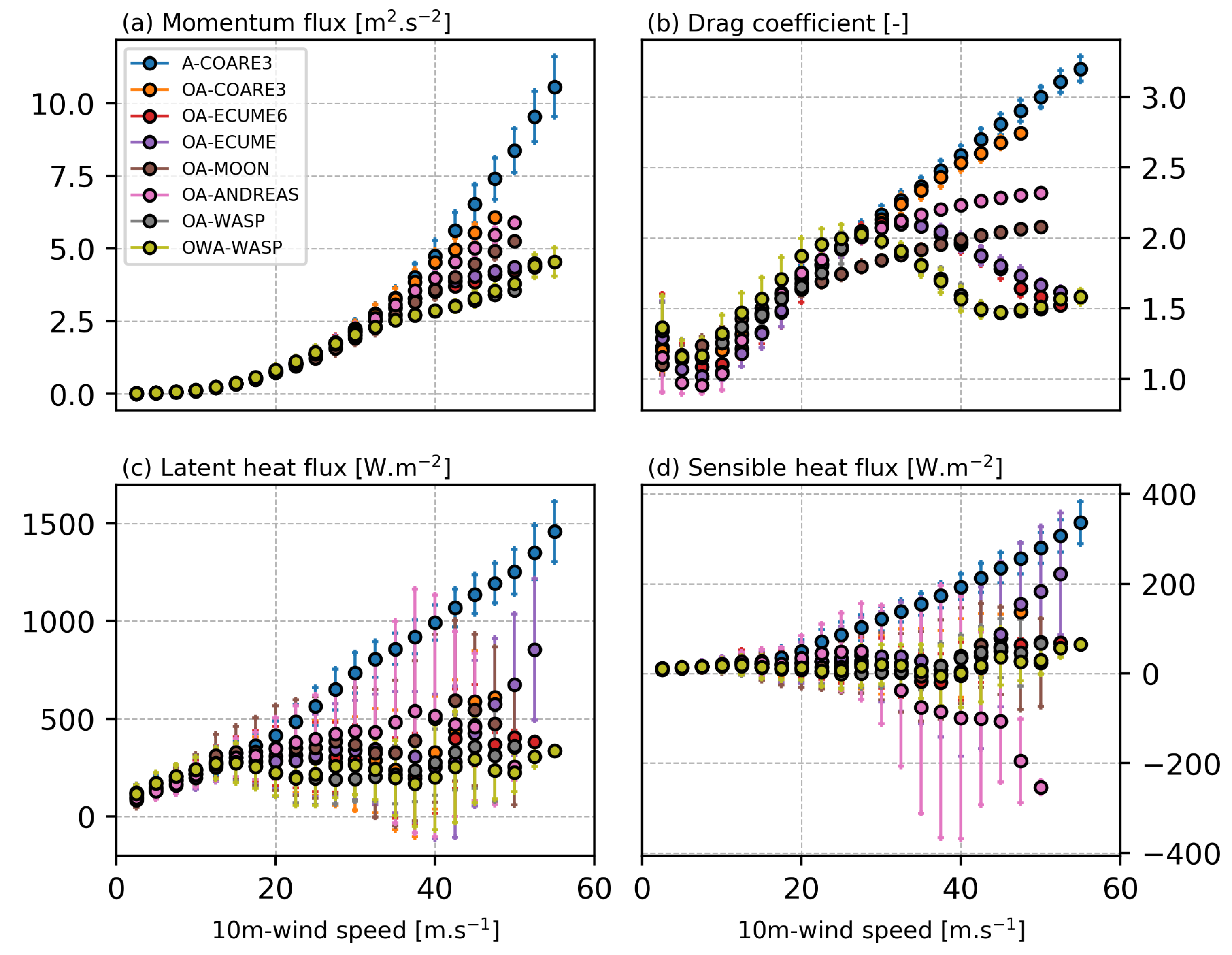
2.2. Coherent Parameterizations for Tropical Cyclone Modeling

In the framework of this program, considerable attention has been paid to the development of the aerosol–microphysics–radiation interactions in tropical storms. The OWA coupled system described in Section 2.1 enables the use of variables from another compartment of the coupled system but coherently computed with respect to the two other compartments. For example, the OWA system enables the computation of sea salt aerosols emission in the SurfEx surface model using the wind field from the atmospheric model, the sea surface temperature and salinity from the ocean model, and the significant wave height from the wave model. If a wave model is not considered and coupled inline, the significant wave height must be interpolated from an external model (offline simulation of a wave model, interpolation from ECMWF analysis, or prescription of a constant value). However, it can lead to sea spray particles spatial distribution incoherent with the wind and wave fields [23].

In the SurfEx model, a sea salt aerosol emission parameterization [58] has been introduced. If the Meso-NH atmospheric model is used, these particles are implemented in the ORILAM aerosol scheme [59,60] and experience transport by advection, sedimentation and turbulence, and dry or wet deposition. These aerosols can serve as cloud condensation nuclei (CCN) thanks to the coupling between the ORILAM aerosol scheme and the LIMA 2-moment microphysics scheme [33,61]. The relatively high computational cost of the aerosol scheme prevents it from being implemented in an operational model such as AROME. Therefore, if the AROME atmospheric model is used, the sea salt aerosols emitted in the SurfEx model are directly coupled with the LIMA microphysics scheme. The direct implementation of sea salt aerosols into the 2-moment microphysics scheme does not allow for the consideration of a complex dimensional distribution, the atmospheric formation of new particles (nucleation), and the aging of aerosols (coagulation, gas-particles interactions), but their spatial distribution coherent with the wind and wave fields is preserved.

Additional developments related to ice microphysics are also going on. Several prognostic variables representing different ice crystal habits have been implemented in LIMA to better represent the diversity of ice crystal properties in clouds and cloud-radiation interactions. Two crystal habits are considered to represent the primary habits (columns and plates) formed between 0 and −20 ${}^{\circ }$C. Two additional variables are necessary to represent the transition between primary habits [62] and the polycrystals generally encountered at temperatures below −20 ${}^{\circ }$C [63]. Different coefficients of the mass-diameter and fall speed-diameter relationships and of the capacitance are attributed to each ice crystal variable, and microphysical processes are computed accordingly. In each grid mesh, the ice crystal effective radius is computed from the prevailing ice crystal habits in terms of number concentration and is passed to the radiation scheme (Figure 1). This enables a consistent treatment of the aerosol–microphysics–radiation interactions in clouds.

3. Some Examples of Coupled Ocean–Atmosphere Modeling of TCs in the SWIO

The coupled system described in Section 2 has been used to simulate several TCs that evolved in the SWIO with the aim to progress on the physical processes involved in TC development and intensification and to produce realistic wind, precipitation, and swell fields over the SWIO territories. The objective of this section is to illustrate the OWA coupled system and its modularity and the consistence of the models and physical parameterizations. Several observational data obtained in the framework of the RNR-CYC program [15] are used to validate the coupled model. The best-track database from RSMC La Réunion is used to evaluate the track and intensity of each modelled TC. In the SWIO, the maximum wind speed ($V_{MAX}$) used to classify the storm intensity is calculated over a 10-min period. When $V_{MAX}$ is between 14 and 16 m s${}^{-1}$, a storm is called a Tropical Depression (TD). Although it has not been given a name at this stage, it is registered in operational TC databases and starts to be tracked by RSMC La Réunion. A storm is given a name when it reaches the stage of Moderate Tropical Storm (MTS, $V_{MAX}$ ≥ 17 m s${}^{-1}$), which is generally considered as the time corresponding to the completion of the cyclogenesis. Storms reaching MTS intensity, hereafter referred to as Cyclogenetic Storms (CS), are classified into four more categories according to their lifetime maximum intensity (LMI): Strong Tropical Storms (STS, 28 ≤ $V_{MAX}$ ≤ 32 m s${}^{-1}$), Tropical Cyclones (TC, 33 ≤ $V_{MAX}$ ≤ 45 m s${}^{-1}$), Intense Tropical Cyclones (ITC, 46 ≤ $V_{MAX}$ ≤ 59 m s${}^{-1}$), and Very Intense Tropical Cyclones (VITC, $V_{MAX}$ > 60 m s${}^{-1}$).

3.1. Numerical Setup of the Simulations

In this section, we define the basic configuration of each model used in the coupled modeling platform. The model configuration for each simulation is summarized in

Table 1. Summary of the models used in the coupled simulations. The domain size and horizontal grid spacing ($\Delta x$) used for each model and each TC is indicated. If two nested domains are used (as for Dumile), D1 and D2 represent the outer and inner domains, respectively. COARE, ECUME6, and WASP refer to the air–sea flux parameterizations of Fairall et al. [47], Belamari [48] and Sauvage et al. [64], respectively. For the microphysics, ICE3 and LIMA mean that the 1-moment microphysics ICE3 scheme [65] and the ORILAM-LIMA coupling [33] are used, respectively.

Tropical Cyclone	Domains		Atmosphere		Surface	Wave	Ocean	Duration
	nb of Points	$\mathbf{\Delta }\mathit{x}$	Model	Microphysics	OA Flux
Dumile (2013) [33]	D1: 450 × 450	8 km	Meso-NH	LIMA	COARE	-	-	51 h
	D2: 400 × 584	2 km
Bejisa (2014) [23]	600 × 500	2 km	Meso-NH	ICE3	COARE	WW3	CROCO	42 h
Bejisa (2014) [66]	600 × 500	2 km	Meso-NH	ICE3	ECUME6	-	NEMO	42 h
Bejisa (2014) [67]	1000 × 800	3 km	Meso-NH	ICE3	COARE	-	CROCO	120 h
Fantala (2016)	1250 × 750	2 km	Meso-NH	ICE3	COARE	WW3	CROCO	240 h
Herold (2019)	1600 × 900	2.5 km	AROME	ICE3	ECUME6	-	NEMO	4 × 48 h
Idai (2019)	750 × 800	2 km	Meso-NH	LIMA	WASP	WW3	CROCO	96 h

.

For the Meso-NH atmospheric model, a single domain with 2 km horizontal grid spacing is used. Seventy vertical levels are specified with increased resolution in the lower levels. Several options for microphysics are available in Meso-NH. Herein, two parameterizations are used (see Table 1): the microphysics is described by the 1-moment bulk microphysics scheme called ICE3 [65] predicting the mixing ratio of cloud droplets, raindrops, pristine ice, snow/aggregates, and graupel or by the 2-moment microphysics scheme LIMA coupled to the ORILAM aerosol scheme as described in Section 2.2. The turbulence parameterization is based on a 1.5 order closure [68] with vertical turbulent flux computations and using the mixing length of Bougeault and Lacarrere [69]. A shallow convection scheme is used based on mass-flux computations [70]. The ECMWF radiative scheme [71] including the Rapid Radiative Transfer Model (RRTM) parameterization [72] is used. The initial and lateral boundary conditions are specified by the 6-hour ECMWF/IFS operational analysis (https://www.ecmwf.int/, accessed on 27 May 2021). If the ORILAM-LIMA coupling is used, aerosol analysis from CAMS (https://atmosphere.copernicus.eu/, accessed on 27 May 2021) [73] are used as initial and boundary conditions of the aerosol and microphysics schemes in Meso-NH [33].

For the AROME atmospheric model, a single domain with 2.5 km horizontal grid spacing is used. Ninety vertical stretched levels are specified with the first level at 5 m and the top of the model at 10 hPa. The initial and lateral boundary conditions are taken from hourly ECMWF/IFS operational forecasts. The physical parameterizations used herein are the ones used in AROME-France as specified in Seity et al. [38], including the 1-moment microphysics scheme ICE3 [65] and the ECUME (Exchange Coefficients from Unified Multi-campaigns Estimates) parameterization for air–sea fluxes [48].

The SurfEx surface model has the same horizontal resolution and number of points as the atmospheric model (Meso-NH or AROME). It is initialized by the ECMWF/IFS operational analysis. The land–atmosphere interaction scheme ISBA [44] is used. Several parameterizations for sea surface exchanges are available in SurfEx [47,48,64,74,75]; the parameterization used in each simulation is indicated in Table 1.

The grid covered by WW3 is the same as that of the atmospheric model with a horizontal grid spacing of 2 km. The global time step is 100 s. The spectral discretization of WW3 is 24 for the direction and 32 for the frequency. For the present study, the third-order Ultimate Quickest scheme [76] with the Garden Sprinkler correction was used to avoid this numerical artifact due to the discrete directions of wave propagation. The wind–wave interaction source term of Ardhuin et al. [77] was used. This parameterization is built around a saturation-based dissipation, reducing the unrealistically large drag coefficients under high winds. Nonlinear wave–wave interactions were modeled using the Discrete Interaction Approximation (DIA) [78]. Additionally, depth-induced wave breaking [79] and bottom friction source terms [80] were used. In order to allow the downscaling from the global "Modélisation et Analyse pour la Recherche Côtière" analyses (MARC; http://marc.ifremer.fr/, accessed on 27 May 2021), a 7-day simulation with the wave model alone is performed before the fully coupled simulation.

The domain for the CROCO oceanic model is the same as the atmospheric and wave models with horizontal grid spacing of 2 km. The domain consists of 32 vertical levels with increased resolution near the surface. A “time-splitting” scheme is used with baroclinic and barotropic time steps of 100 s and 2 s, respectively. The advection scheme is third-order upstream biased [81]. Subgrid-scale vertical mixing is solved by the nonlocal K-profile parameterization scheme [82]. The model is initialized and forced at the lateral boundaries every day with global analyses (1/12${}^{\circ }$) provided by Mercator Ocean (https://www.mercator-ocean.fr/en/, accessed on 27 May 2021).

The domain for the NEMO oceanic model is the same as for the atmospheric domain with horizontal grid spacing of 1/12${}^{\circ }$ (about 9 km) and 50 unevenly spaced vertical levels. A time step of 360 s is used for the dynamic. The vertical mixing is a turbulent kinetic energy closure scheme based on Gaspar et al. [49] and modified by Madec et al. [83]. The split-explicit free surface formulation follows the one proposed by Shchepetkin and McWilliams [52]. In the same way as CROCO, NEMO is initialized and forced at the lateral boundaries every day with the global analyses from Mercator Ocean global model PSY4 [84].

3.2. Modeling Studies of Tropical Cyclones Dumile (2013) and Bejisa (2014)

Several parts of the modeling platform have been independently evaluated in the last few years. These published studies are not detailed hereinafter but a short statement of the main findings is given in this section.

A first evaluation of the aerosol–microphysics coupling was performed through the simulation of TC Dumile (2013) [33] that impacted La Réunion in January 2013. The importance of explicitly taking into account sea salt aerosol emissions associated with high winds and waves in TCs was shown to be a critical point for simulating the track, intensity, and structure of long-lasting systems that need to generate their own CCN.

Several modeling studies of TC Bejisa that passed in the neighborhood of La Réunion in January 2014 have been performed with the modeling platform described in Section 2. Using the Meso-NH/WW3/CROCO coupled system, Pianezze et al. [23] showed that online coupling with a wave model is important to obtain a spatiotemporal and size distribution of sea salt aerosol particles coherent with the wind and sea state fields. Bielli et al. [66] evaluated the sensitivity of Bejisa simulation to the degree of ocean–atmosphere coupling. They showed that using a 1D coupling (Meso-NH coupled to a 1D ocean mixed layer model) does not enable to reproduce the intensity and structure of surface ocean cooling compared to composite observations, while a 3D coupled model (Meso-NH coupled to the 3D NEMO model) does. Finally, an ocean–atmosphere configuration with km-scale grid spacing was implemented to investigate how the characteristics of a typical TC like Bejisa would evolve in the context of climate change [67]. The pseudo global warming method was used to construct future environments: perturbations computed from six Coupled Model Intercomparison Project 5 (CMIP5) climate models were added to historical analyses from ECMWF. This high resolution study complements the climate projections at the basin scale realized in the framework of RNR-CYC program and described in Section 4.

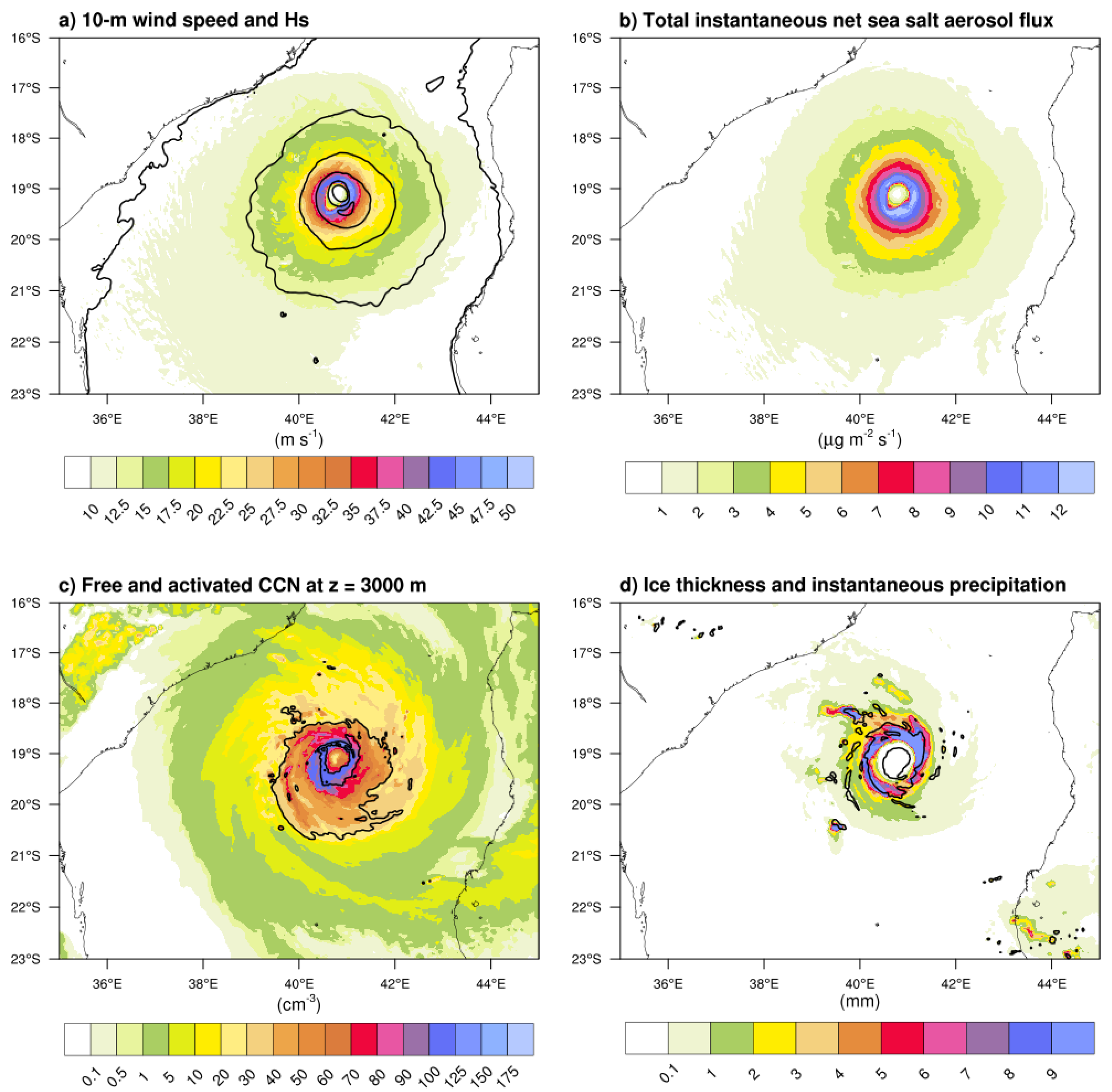
3.3. Tropical Cyclone Fantala (2016)

Fantala (2016) is the second most intense TC ever observed in the SWIO with 10-min sustained wind speed reaching 69 m s${}^{-1}$ on 17 April 2016 at 18 UTC. Fantala moved over and devastated the Farquhar group of Seychelles on 17 April with wind gusts estimated at 96 m s${}^{-1}$. Fantala exhibits a very unusual track turning back twice during its 16 days lifecycle (Figure 2). This uncommon track makes Fantala a perfect candidate to evaluate the impact of air–sea flux parameterization on the storm development.

The simulation of TC Fantala was performed with Meso-NH/SurfEx, WW3, and CROCO on a single domain located between 44.54${}^{\circ }$ E and 67.64${}^{\circ }$ E and between 17.66${}^{\circ }$ S and 4.18${}^{\circ }$ S (Table 1). The simulation starts on 14 April 2016 00 UTC and lasts 240 h encompassing the two U-turns of Fantala. The simulation matches the basic configuration described in Section 3.1, but several additional simulations have been performed to investigate the impact of air–sea flux on the evolution of this system. These simulations differ by the degree of OWA coupling and the air–sea flux parameterization (

Table 2. Summary of the simulations of TC Fantala. A, OA, and OWA stand for Atmosphere, Ocean–Atmosphere, and Ocean–Wave–Atmosphere simulations, respectively.

Simulation	Meso-NH/SurfEx	WW3	CROCO	Air–Sea Flux Param.
A-COARE3	X	-	-	COARE3 [47]
OA-COARE3	X	-	X	COARE3 [47]
OA-ECUME	X	-	X	ECUME [48]
OA-ECUME6	X	-	X	ECUME6 [48]
OA-MOON	X	-	X	MOON [74]
OA-ANDREAS	X	-	X	ANDREAS [75]
OA-WASP	X	-	X	WASP [64]
OWA-WASP	X	X	X	WASP [64]

).

Six different air–sea flux parameterizations available in SurfEx have been tested in this study and are basically described hereinafter. The COARE3.0 parameterization [47] is derived from COARE2.6 [85] which was developed from observations of the TOGA-COARE field campaign [86] in the North Pacific. An important update of COARE3.0 is the new formulation of the roughness length that increases when the wind speed exceeds 10 m s${}^{-1}$. However, this parameterization is mainly valid for wind speeds lower than 20 m s${}^{-1}$ due to the lack of observations for high wind conditions. The wave effect is considered through the roughness length [87]. The WASP (Wave Age Stress dependant Parameterization) parameterization [64] is based on the COARE3.0 parameterization but the roughness length computation has been modified to consider the sea state. Since different mechanisms are involved at weak (<5 m s${}^{-1}$), moderate (5–20 m s${}^{-1}$), and high (>20 m s${}^{-1}$) wind speeds, a piecewise continuous description is adopted to describe the Charnock parameter. It enables the representation of the observed decrease of the drag coefficient in strong wind conditions. The ECUME and ECUME6 parameterizations [48] are built upon in-situ air–sea fluxes from different field campaigns. While ECUME is tailored for low to moderate winds, high wind conditions are considered in ECUME6. The turbulent exchange coefficients are computed directly from observations which makes the wave impossible to consider in the roughness length computation. The ANDREAS parameterization [75] is the only parameterization that intends to take into account the effect of sea sprays on sensible and latent heat fluxes through their evaporation in the atmospheric boundary layer. However, this parameterization only uses data up to wind speed of 25 m s${}^{-1}$. Finally, the MOON parameterization [74] is based on wind–wave coupled numerical simulations of ten TCs. A new expression of the roughness length has been derived that limits its increase as soon as the wind speed exceeds 12.5 m s${}^{-1}$.

Whatever the parameterization of air–sea flux used, the simulated tracks are close to the best-track (Figure 2). As soon as the ocean–atmosphere coupling is activated, the position of the U-turns is well simulated, whether in terms of timing (less than 2 h and 6 h deviation from the best-track for the first and second U-turns, respectively) or in terms of position (less than 20 km and 100 km for the first and second U-turns compared to the best-track). The choice of the air–sea flux parameterization has then little impact on the simulated track. This confirms that Fantala’s track is mainly determined by large-scale flow. Nevertheless, after the second U-turn, the coupled ocean–atmosphere simulation with WASP parameterization (OA-WASP, grey line in Figure 2a) differs from the others. The wave field used for this parameterization is a function of the 10-m wind only and is not realistic in this simulation: the coupling with a wave model is necessary if this parameterization is used as shown by the green line in Figure 2 (OWA-WASP). It must also be noted that in case of the atmosphere-only simulation (A-COARE3, blue line in Figure 2a), the position of the first U-turn differs by more than 6 h and 100 km from the timing and position analyzed in the best-track.

Concerning the intensity of the modeled TC (Figure 2b), the choice of the air–sea flux parameterization can have a significant impact. The forced simulation (A-COARE3, blue line) produces a system that remains too intense compared to the best-track despite the two U-turns. It is clear that the A-COARE3 simulation is not able to capture the storm weakening (between 18 April 06 UTC and 19 April 00 UTC) after the first U-turn unlike the other simulations that use an ocean–atmosphere coupled model. This is explained by the absence of cooling under the cyclone. This simulation is a perfect example of the need for ocean–atmosphere coupling to correctly simulate the evolution of TC intensity. Apart from the forced simulation, the other simulations capture the overall trend of intensity variation even if they are not able to reproduce the maximum intensity on 18 April (910 hPa). The OA-ANDREAS simulation (pink line) produces the most intense system, and the closest to the best-track, during the first five days. The other simulations remain relatively close with differences of up to 30% with the best-track.

To quantify the effect of these parameterizations on turbulent fluxes and indirectly on TC intensity, the momentum fluxes, the drag coefficient ($C_d$), and the latent and sensible heat fluxes as a function of the 10-m wind speed are shown on Figure 3 when Fantala reaches its maximum intensity (18 April 2016 at 00 UTC), before its first U-turn. The four parameters show variability for a given 10-m wind speed: this is explained by the effect of the stability of the atmosphere and waves on the turbulent fluxes which varies from one grid point to another.

For the momentum flux (Figure 3a) and the drag coefficient (Figure 3b), all simulations show a similar average value up to 10-m wind speed ∼30 m s${}^{-1}$, which corresponds to the domain of validity of these parameterizations. From 30 m s${}^{-1}$, the average values of the momentum flux and of the drag coefficient start to diverge depending on which parameterization is used. The COARE3.0 parameterization (blue and orange dots and segments) has a drag coefficient that increases with the 10-m wind speed ($C_d$ = 2.6 and 3.0 for 10-m wind speed of 40 and 50 m s${}^{-1}$, respectively) and produces the strongest momentum fluxes (8.5 m${}^2$ s${}^{-2}$ for 10-m wind speed of 50 m s${}^{-1}$). Observations under strong wind conditions show a saturation of the drag coefficient and even a decrease when the wind speed exceeds 40 m s${}^{-1}$ [88]. As expected, the COARE3.0 parameterization does not behave realistically in strong wind conditions. It must be noted that the ocean–atmosphere coupling (OA-COARE3) tends to slightly reduce the momentum flux and the drag coefficients for wind speeds above 37.5 m s${}^{-1}$ when compared to the atmosphere only simulation (A-COARE3). The five other parameterizations reproduce the saturation of the drag coefficient. WASP shows the lowest momentum flux and drag coefficient for wind speeds above 30 m s${}^{-1}$: the momentum flux does not exceed 4.5 m${}^2$ s${}^{-2}$ on average for 10-m wind speed of 50 m s${}^{-1}$, while the drag coefficient reaches a mean minimum of 1.5 for 10-m wind speed of 45 m s${}^{-1}$. The MOON and ANDREAS parameterizations are relatively close in strong wind conditions. For 10-min wind speed of 40 m s${}^{-1}$, the drag coefficient does not exceed 2.35 and 2.1 for ANDREAS (pink dots and segments) and MOON (maroon dots and segments), respectively. The ECUME (purple dots and segments) and ECUME6 (red dots and segments) parameterizations show relatively similar behavior in strong winds, with a decrease of the drag coefficient. For 10-m wind speed of 40 m s${}^{-1}$, the drag coefficient is about 1.65 for these two parameterizations. It thus produces the lowest momentum flux in high wind conditions (∼3.7 m${}^2$ s${}^{-2}$ for 10-m wind speed of 50 m s${}^{-1}$), more than half of the momentum flux encountered in the A-COARE3 simulation. However, the ECUME and ECUME6 parameterizations do not allow for the representation of the waves in the drag coefficient, while this coefficient has been shown to vary depending on the wave’s age [87].

The sensible and latent heat fluxes simulated with the different parameterizations show very large differences for 10-m wind speeds higher than 20 m s${}^{-1}$ (Figure 3c,d). In OA-ANDREAS, both the latent and sensible heat fluxes show large standard deviation (for example, for a 10-m wind speed of 40 m s${}^{-1}$, the latent and sensible heat fluxes are 500 ± 650 W m${}^{-2}$ and −100 ± 270 W m${}^{-2}$, respectively). The latent heat fluxes in OA-ANDREAS are located in the middle of all the latent heat fluxes simulated by the other parameterizations, while the sensible heat fluxes are the lowest with negative mean values for 10-m wind speed higher than 30 m s${}^{-1}$. As for the momentum flux, the A-COARE3 simulation exhibits the largest sensible and latent heat flux with mean values reaching 1000 and 200 W m${}^{-2}$, respectively, for 10-m wind speeds of 40 m s${}^{-1}$. For 10-m wind speeds of 40 m s${}^{-1}$, the coupling with a 3D ocean model reduces dramatically the sensible and latent heat flux (500 and 40 W m${}^{-2}$, respectively, in OA-COARE3). The other simulations exhibit a similar behavior in terms of heat fluxes, except OA-ECUME that diverges from the other simulations (OA-ECUME6, OA-MOON, OA-WASP, OWA-WASP) for wind speeds higher than 45 m s${}^{-1}$ and behaves like OA-COARE3.

As already shown (e.g., [89]), the choice of the air–sea flux parameterization affects the intensity of the cyclone. However, in the case of TC Fantala, the effect of 3D coupling with the ocean has more impact on the intensity after the first U-turn while the choice of the air–sea flux parameterization is essential before the first U-turn. A more advanced analysis is going on to fully understand the air–sea interactions in this complex TC.

3.4. Tropical Cyclone Idai (2019)

In order to demonstrate the importance of consistently considering atmospheric, oceanic, and wave parameters, the OWA coupled system was used to forecast the intense tropical cyclone Idai (2019). TC Idai landed on the region of Beira (Mozambique) on 15 March 2019 (Figure 4a). TC Idai developed during the 2019 regional field campaign and was captured by the Sentinel 1A / 1B acquisitions. The simulation of TC Idai was performed with Meso-NH, WW3, and CROCO on a single domain covering the Mozambique Channel (Table 1). The aerosol–microphysics–radiation interaction described in Section 2.2 is used herein. Aerosol analysis from CAMS (https://atmosphere.copernicus.eu/ accessed on 27 May 2021) [73] are used as initial and boundary conditions of the aerosol and microphysics schemes in Meso-NH as described in Hoarau et al. [33]. The simulation starts on 11 March 2019 00 UTC and lasts 96 h, until TC Idai makes landfall in the region of Beira.

Figure 4 shows the track and intensity of TC Idai as analyzed in the RSMC La Réunion best-track and simulated by Meso-NH/WW3/CROCO. The modeled track matches very well the best-track during the first 48 h (Figure 4a). On 13 March at 00 UTC, the cyclone in the model starts to accelerate which causes a landfall occurring 6 h in advance compared to the best-track. Despite a 7 hPa underestimation at the initial state, the model manages to represent the overall intensity tendency during the first 42 h (Figure 4b). Idai experienced an eyewall replacement cycle on 12 and 13 March which is not captured by the model leading to an overestimation of the intensity. On 14 March at 00 UTC, Idai reached a maximum of intensity (940 hPa) rather well reproduced by the model (948 hPa). During the last 12 h of the simulation, the intensity collapses due to the 6-hour delay in landfall.

Figure 5 shows horizontal cross sections of TC Idai on 12 March 2019 at 18 UTC simulated by the OWA system. At this date, Idai moves to the west, and its intensity is analyzed at 966 hPa by RSMC La Réunion vs. 962 hPa for the modeled TC. The 10-m wind speed (Figure 5a) exceeds 40 m s${}^{-1}$ all around the eyewall and exhibits two maxima (45 m s${}^{-1}$) at the south-western and at the north-eastern sides of the system. The significant wave height ($H_S$) exceeds 8 m all over the eyewall. Its maximum (10.5 m) is located in the southeastern region of the cyclone (i.e., in the right-front area relative to the cyclone track). $H_S$ values higher than 6 m extend over more than 300 km from the center of the cyclone, i.e., over the most part of the Mozambique channel. The strong surface winds and the high $H_S$ are the main parameters involved in the emission of sea salts aerosols. Sea salt aerosol mass flux higher than 10 μg m${}^{-2}$ s${}^{-1}$ is found in the eyewall at 20 m above sea level (asl) (Figure 5b). Values higher than 12 μg m${}^{-2}$ s${}^{-1}$ are located in the southern part of the eyewall where the maximum wind speed and wave height are encountered. The sea salt aerosol mass flux remains significant (>1 μg m${}^{-2}$ s${}^{-1}$) in the region where the 10-m wind speed and $H_S$ exceeds 10 m s${}^{-1}$ and 6 m, respectively. These values are probably underestimated since the parameterization of sea salt emission used in SurfEx [58] mainly considers the generation of submicronic sea salt particles. Supermicron particles are also generated but there are large uncertainties concerning their generation function (see Figure 6 in [90]). However, due to their large size, even if their number concentration is low, their contribution to the mass flux is important. In the ORILAM aerosol scheme, sea salt aerosols with dry diameter greater than 80 nm represent the CCN concentration reported in Figure 5. At 3000 m asl, high number concentration (between 30 and 125 cm${}^{-3}$) of available CCN is modeled in the inner core of the system (Figure 5c). These concentrations are strongly inhomogeneous due to the balance between the sea salt aerosol emission, the vertical transport, and the precipitation scavenging that occurs within the convective cells. Maximum values of activated CCN (∼10 cm${}^{-3}$) are found in the eyewall at this altitude. During the 2-month field campaign, the Boreal unmanned airborne system equipped with meteorological, aerosol, sea state, and turbulence instruments, made several flights in a large area around La Réunion [15]. Boreal measurements showed aerosol concentrations (diameter > 0.3 μm) in the range 50–150 cm${}^{-3}$, increasing with wind speed and wave height (see Figure 16 in [15]). This range of aerosol concentrations was sampled for wind speed between 2.2 and 13.5 m s${}^{-1}$, wave height between 2 and 3.7 m, and below 200 m asl. At 60 m asl, the coupled simulation displays available CCN concentrations between 100 and 150 cm${}^{-3}$ in the region with wind speed ∼13 m s${}^{-1}$ and wave height ∼3.5 m (not shown) which is comparable to observed values. The total ice thickness is higher than 9 mm in the south-western and north-eastern part of the eyewall (Figure 5d). Instantaneous precipitation higher than 10 mm h${}^{-1}$ is found colocated with the high value of total ice thickness in the eyewall, showing ice phase precipitation in this region.

As shown in Bousquet et al. [15], one important achievement of RNR-CYC lied in the collection of numerous space-borne synthetic aperture radar (SAR) observations within TC developing in the SWIO. As shown in the following, such data can be particularly useful to evaluate TC simulations made in the frame of the project but also to improve RSMC La Réunion real-time or post-event analyses of TC intensity and improve model forecast from assimilating SAR observations into high-resolution NWP systems [91]. During TC Idai, two exploitable SAR images were collected directly within the core of the storm, including one slightly before its landfall in Beira, on 14 March 2019 at 16:05 UTC. This SAR image (Figure 6a) locates the center of TC Idai 90 km to the east of Beira. The retrieved surface wind field shows wind speed values in the eyewall between 35 and 46 m s${}^{-1}$, with a reduced region with maximum wind speed of 46 m s${}^{-1}$ in the northeastern part of the eyewall. On 14 March at 18 UTC, the minimum sea level pressure and the maximum 10-min sustained wind speed were estimated by the best-track from RSMC La Réunion at 955 hPa and 42 m s${}^{-1}$, respectively. Due to a faster translation speed in the simulation compared to the best-track from 13 March at 00 UTC, the simulated TC is located ∼80 km offshore the Mozambique coast on 4 March around 14 UTC. The modeled system is ∼6 h in advance and lands slightly too south (∼20 km) compared to the observations (Figure 5a). The OWA simulation at 13 UTC produces higher wind speed in the eyewall (>46 m s${}^{-1}$, with a maximum of 60 m s${}^{-1}$; Figure 6b) than the SAR retrieval at 16 UTC. However, the 34 m s${}^{-1}$ wind extension is similar in the simulation and the SAR retrieval (90–100 km). Despite a landing in Mozambique a few hours in advance and with a slightly overestimated intensity, the OWA system is able to reproduce the overall evolution of TC Idai during this 4 day simulation. However, the model was not able to capture the eyewall replacement cycle. This deficiency will be investigated, in particular the potential impact of the microphysics parameterization on the eyewall replacement cycle development [92,93].

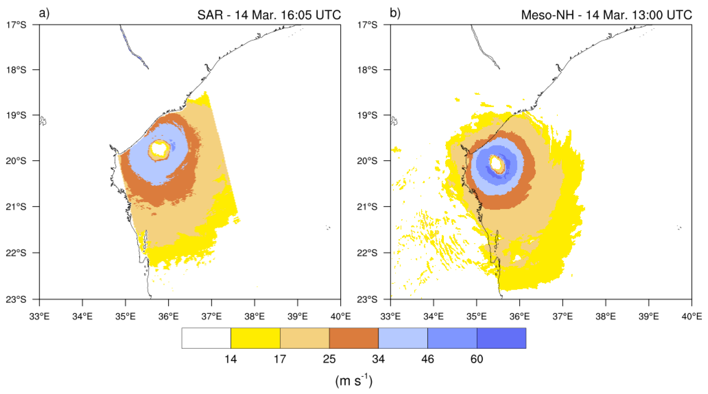
3.5. Tropical Cyclone Herold (2020)

3.5.1. Storm Description and Model Simulations

The intense tropical cyclone Herold (2020) initiated as a tropical depression located north-east of Madagascar on 12–13 March 2020. This system, the second most intense storm of the 2019–2020 TC season in the SWIO basin, initially moved towards Madagascar while slowly intensifying before stopping off-shore the coast on 14 March, where it remained stationary for about 24 h (Figure 7). It then turned around to head south-east and underwent a rapid intensification to reach ITC stage in the morning of 17 March, with 10-min averaged sustained winds of ∼46 m s${}^{-1}$ and wind gusts of up to 64 m s${}^{-1}$. The intensification phase of TC Herold was sampled by one of the two space-borne SAR deployed onboard ESA’s Sentinel-1 satellites and two of the sea turtles deployed in RNR-CYC (see Part 1, [15]). Although it did not impact inhabited territories, TC Herold is thus a particularly interesting case to evaluate the potential of the novel observations deployed in this project.

TC Herold was simulated for 126 h with the OA coupled system AROME/NEMO from 13 March 2020 at 12 UTC. This coupled model, which prefigures the future operational NWP system that will soon be used by RSMC La Réunion for TC forecasting in the SWIO, was run for four periods of 48 h, respectively initialized on March 13 (HR1), 14 (HR2), 15 (HR3), and 16 (HR4) at 12 UTC, with ocean cycling every 24 h (i.e., runs HR2/3/4 start from the ocean state of the 24 h forecast of the previous coupled run). For HR1, NEMO was initialized from Mercator-Ocean operational model (also known as Glo12), which also provided lateral boundary conditions every day. AROME was initialized from ECMWF’s IFS operational NWP system, which also provided lateral boundary conditions every 6 h. In order to reduce the model spin up and be able to already produce small scale features at initiation time $T_0$ in the model, ECMWF large-scale atmospheric fields (temperature, wind, humidity, and surface pressure) valid at $T_0$ were combined with a 6-h AROME forecast initialized at $T_0-6$ h [94].

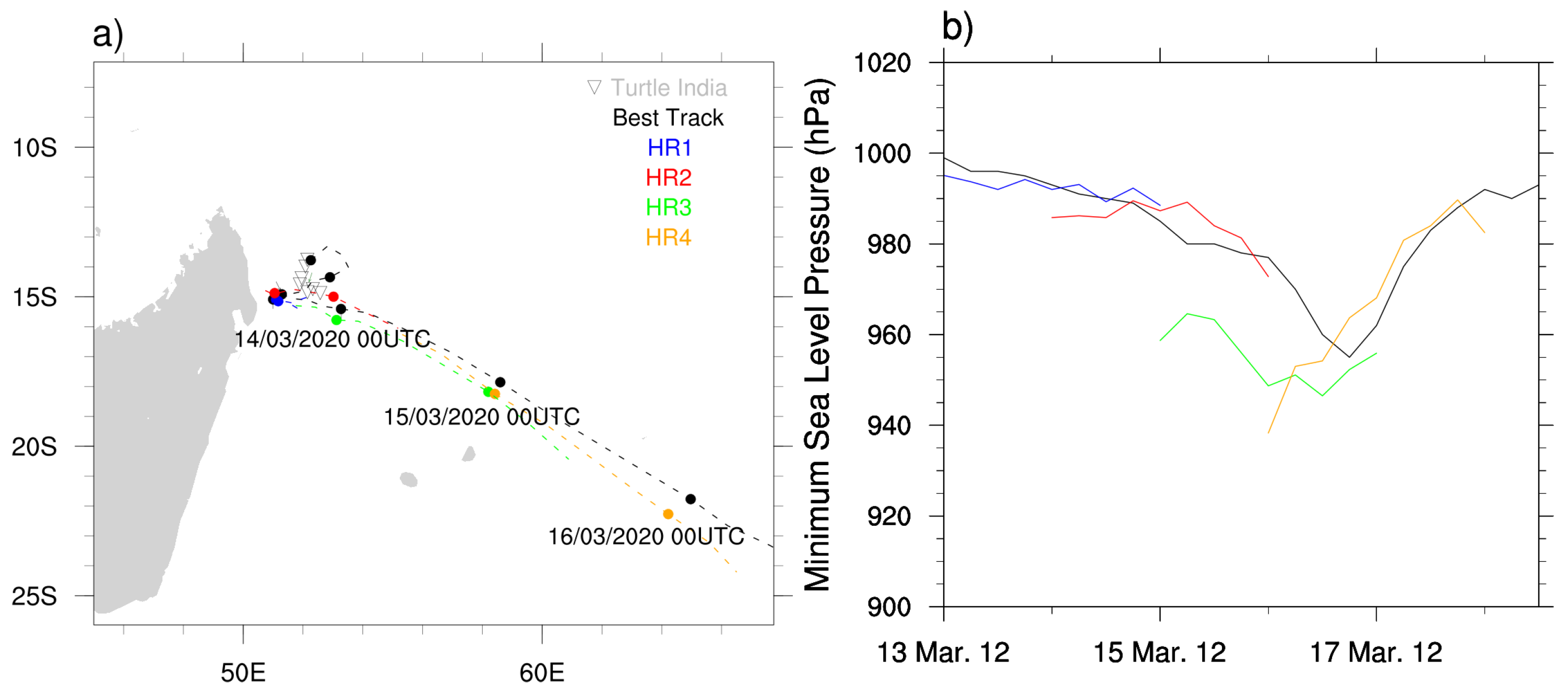
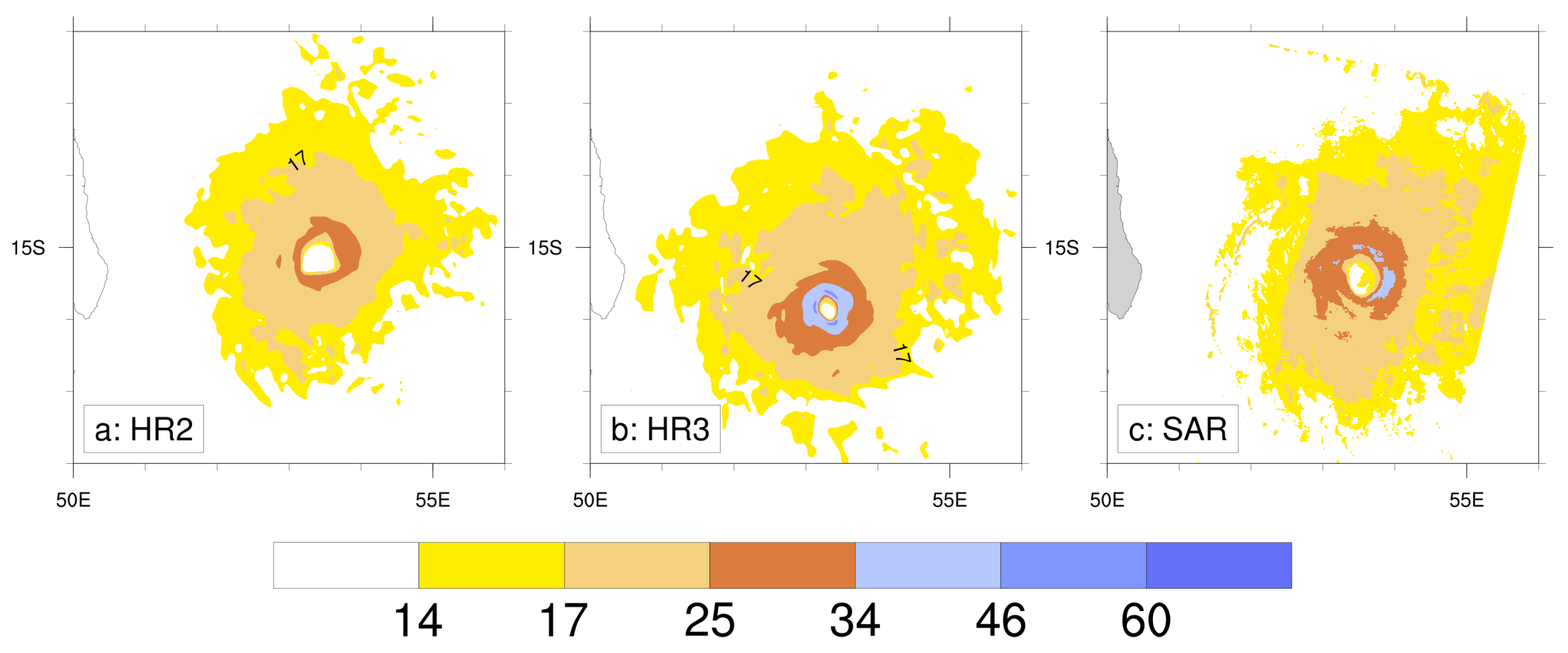
3.5.2. TC Track and Intensity Forecasts

Figure 7 shows the track and intensity (MSLP) of TC Herold as analyzed in RSMC La Réunion best-track and simulated by AROME/NEMO between 13 and 18 March 2020. Runs HR1 (blue line) and HR2 (red line) show good agreement with best-track data both in terms of trajectory and intensity, meaning that the coupled model was able to correctly reproduce the cyclogenesis of the system. For run HR3 (green line), the storm intensity simulated by AROME/NEMO is however significantly overestimated following an overestimation of the MSLP of ∼25 hPa at initialization time. The mean rate of intensification over time is nevertheless relatively consistent with that observed in the best-track (∼25 hPa in 36 h), as is the time when the system reached its maximum intensity (947 hPa on 17 March at 00 UTC vs. 955 hPa on 17 March at 06 UTC). For the last run (HR4, yellow line), the intensity at initialization time is even more erroneous, with an error in initial MSLP of nearly −35 hPa with respect to best-track data. This strong initial bias is nevertheless quickly cancelled, with modeled intensities beginning to precisely match best-track data after 18 h of simulation. The initial positions of the storm in the two latter runs are also slightly shifted southwards (∼20 km) with respect to best-track data with positioning errors slightly increasing over time to reach ∼80 km at the end of the simulations. Despite these errors, the simulation of TC Herold by AROME/NEMO can be considered as satisfactory. Hence, the coupled model is shown to simulate the cyclogenesis and the first smooth intensification phase of the TC with little discrepancies (runs HR1 and HR2). Despite a significant overestimation of the initial TC intensity in runs HR3 and HR4, the model is also able to gradually adjust itself to eventually match reference measurements.

As mentioned previously, comparisons to best-track data allow for the evaluation of the performance of the model in a broad sense, but SAR data collected in RNR-CYC represent a rare opportunity to more precisely evaluate intensity and structure forecasts over the open ocean as well as to refine comparisons with RSMC La Réunion analyses. In this regard, a comparison between SAR-derived observations made in TC Herold on 16 March 2020 at 02 UTC, i.e., more or less when the storm reached TC intensity (33 m s${}^{-1}$), and simulated surface winds at the same time are shown in Figure 8.

According to SAR-derived wind data (Figure 8c), the eye of the system at observation time was more or less circular with a diameter of ∼40 km, but the eyewall was not yet well structured and was showing a weakness in the southern quadrants. The maximum intensity was observed in the eastern quadrant of the eyewall with surface wind speed of ∼34 m s${}^{-1}$. Corresponding 10-m surface winds inferred from model simulations HR2 (38-h forecast lead time) and HR3 (14-h forecast lead time) are shown in Figure 8a,b, respectively. In good agreement with pressure data shown in Figure 7, the structure and intensity of the TC simulated in run HR2 show good consistency with satellite data. The simulated TC eye has both proper dimension and position, and maximum simulated surface winds (∼32 m s${}^{-1}$) are located in the eastern quadrant of the eyewall. While the 34 m s${}^{-1}$ wind extension (brown colour, hurricane force) is slightly more compact in the simulation, the 25 m s${}^{-1}$ (beige colour, storm force) and 17 m s${}^{-1}$ (yellow colour, gale force) wind extensions both match observations very well. As expected from Figure 7, stronger discrepancies can be noticed for run HR3 (Figure 8b). Compared to SAR data, the location of the storm center is then shifted southwards by about 40–50 km and surface wind values are significantly higher, with maximum wind speed of ∼46 m s${}^{-1}$ all the way around the eye (vs. 34 m s${}^{-1}$ in SAR data). The TC eye simulated by the model is also significantly smaller than in the SAR observations and appears completely enveloped by the eyewall, which is indicative of a more organized and intense system. Despite significantly stronger winds near the core of the system, hurricane, storm, and gale force wind extensions nevertheless match observations quite well.

Such differences in behavior between successive model runs are not uncommon but do nevertheless pose problems to TC forecasters who need relatively stable forecasts over time to make their predictions. While the comparisons with the best track data might suggest that the model run HR3 is unrealistic, the comparison with SAR-derived observations tempers this impression and shows that the overall structure of the system was actually well simulated by the AROME/NEMO modeling system.

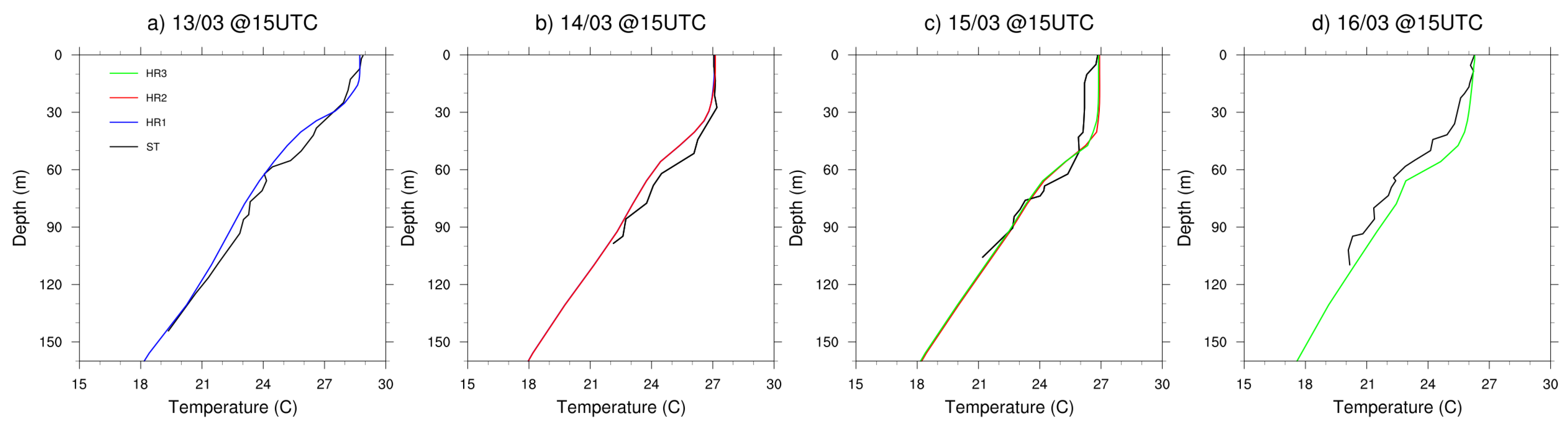
3.5.3. Ocean Temperature Forecasts

Because Earth observing satellites cannot provide SST measurements below TCs due to their associated large cloud cover, a precise validation of ocean model temperature forecasts in cyclonic conditions necessarily requires the availability of in-situ data. As oceanic sensors such as ARGO drifters or moored buoys are sparse in the SWIO, biologging data collected by sea turtles (ST) in the frame of RNR-CYC provide a fantastic possibility to investigate potential changes in surface and subsurface ocean temperature fields under cyclonic conditions. Two of the sea turtles equipped with temperature-depth ARGOS tags released during this program have been able to collect temperature data within or in the immediate vicinity of TC Herold [15]. One animal (ST Tom) has been located a few hundreds km away from the storm for about one week (allowing to sample the overall oceanic environment away from the TC core), and the second one (ST India) remained trapped for about 4 days (13–16 March) in the immediate vicinity of the TC core. While surface temperature data collected by ST India during this period can be used to investigate the temporal evolution of the SST field in the vicinity of TCs (see Figure 10 in [15]), vertical profiles of ocean temperature reconstructed from sea turtles observations also provide a rare opportunity to investigate the performance of coupled ocean–atmosphere models in cyclonic conditions.

Figure 9 presents comparisons between temperature profiles simulated by the AROME/ NEMO coupled system and observed by ST India from 13 to 16 March at 15 UTC. In order to reconstruct ocean temperature profiles from ST-borne observations, temperature-depth measurement pairs collected every 5 min by ST India were aggregated over a period of 3 h centered on 15 UTC. NEMO temperature profiles forecasted from the three model runs encompassing this 4-day period (HR1-3) were extracted at the same time at the grid point closest to the observations. Knowing that sea turtles move at most 2 to 3 km per hour [39], one can thus consider that all sea turtles data used to reconstruct a given vertical profile are collected within the same NEMO column (1/12${}^{\circ }$ horizontal resolution).

As expected, the SST in the vicinity of the TC core is found to decrease significantly during the investigated 72-h intensification period of the storm. The evolution of SST, which dropped from 29 ${}^{\circ }$C on 13 March (Figure 9a) to 26 ${}^{\circ }$C on 16 March (Figure 9d), was well captured in the three model runs. On 13 (Figure 9a, run HR1, blue line) and 14 (Figure 9b, run HR2, red line) March, the observed vertical temperature profiles were also well reproduced by the coupled model, especially in the ocean mixed layer (OML, ∼0–50 m depth on average). The next two days, important discrepancies can however be noticed compared to ST observations. On 15 March (Figure 9b), temperatures are overestimated by ∼1 ${}^{\circ }$C throughout the OML in both runs HR2 and HR3 (green line). As the initialization of ocean fields in simulation HR3 comes from NEMO HR2 outputs valid only 3 h before, observed similar profiles are expected, but these differences are further exacerbated 24 h later (HR3, 27-h forecast lead time). Based on these comparisons, the coupled system is able to properly simulate the surface cooling in the vicinity of the TC but does not seem able to reproduce the temperature drop in the OML during the rapid intensification period of the system. This behavior may be related to an insufficient vertical resolution of the model or to a too strong mixing. Additional simulations of TCs for which ST-borne measurements will be available should be performed to extend the evaluation of the oceanic part of the modeling platform.

4. Climate Projection of Tropical Cyclone Activity in the SWIO

It is commonly accepted that the predicted increase in TC intensity will be related to the increase in atmospheric moisture content resulting from higher SSTs [7,95,96,97,98]. However, no real consensus exists yet regarding the evolution of TC frequency and the underlying physical processes in the context of global warming. Bengtsson et al. [99], Bengtsson et al. [100] and Sugi [101] hypothesized that the number of cyclogenesis in the future will mostly depend on changes in large-scale upward mass flux driven by synoptic circulation. Emanuel et al. [102] and Emanuel [103] suggested that the decrease in TC frequency could be rather related to an increase in the saturation deficit in the middle troposphere as well as temperature modulation in the upper troposphere.

Most recent studies that investigate the impact of global warming on frequency, intensity, and precipitation of tropical storms and cyclones are based on the analysis of climate simulations carried out within the framework of the 5th phase of the Coupled Model Interception Project (CMIP5). As the spatial resolution of CMIP5 experiments is generally too coarse (1${}^{\circ }$ at best) to accurately capture the full life cycle of low-pressure tropical systems, such simulations are not suitable for studying the early stages of the development of TCs in a future climate [104,105]. Although the next phase of the CMIP project (also known as CMIP 6), which includes a few model runs at 50 km, will open up new perspectives on this subject, some climate centers have already begun to conduct high-resolution climate experiments (ranging from 6 to 50 km in horizontal grid spacing) to assess the evolution of cyclonic activity on a regional scale as well as to investigate potentially different trends from one cyclonic basin to another, (e.g., [10,12,13,106]). The results of these studies have mostly confirmed those obtained from CMIP5 models and pointed to a general decrease in TC frequency together with a more or less significant increase in TC intensity and, in some cases, TC-related precipitation [10].

Indeed, while regional and global climate models enable identifying the favored regions of cyclogenesis and occurrence of tropical storms and cyclones at the basin scale, a better spatial resolution and more advanced physical schemes are needed to reproduce the intensification mechanisms and the behavior of tropical systems at landfall. One of the goals of the climate component of RNR-CYC was thus to evaluate the future evolution of TC activity in the SWIO. While high-resolution simulations performed with global models are used to anticipate the global evolution of the TC activity [13], a pseudo global warming procedure is implemented in the coupled OWA model described in Section 2 to evaluate the modifications of the TC structure and impacts in a modified oceanic and atmospheric environment [67].

Cattiaux et al. [13] used high-resolution experiments performed with a rotated-stretched configuration of Météo-France Coupled Global Climate Model (CNRM-CM) to estimate projected changes in cyclonic activity over the South Indian Ocean near the end of the century. The model predicted a 20% decrease in TC frequency together with an increase of TC intensity and a slight shift of TC trajectories towards the poles, as already observed in previous studies [107,108]. In the following we use the high-resolution global climate simulations already used in Cattiaux et al. [13], and specifically made for RNR-CYC, to investigate potential changes in the frequency and intensity of TCs in the SWIO over the period 2051–2094.

4.1. Data and Methodology

4.1.1. CNRM-CM Model Data

This study is based on present-day (1971–2014, hereafter referred to as ARP-P) and future (2051–2094, ARP-F) atmosphere-only experiments performed by Cattiaux et al. [13] using the CNRM-CM climate model in its rotated-stretched configuration [6,106]. This particular configuration, routinely used by Météo-France for operational forecasting applications in Europe with ARPEGE (the atmospheric component of CNRM-CM), allows increasing horizontal resolution over a given region of interest (the pole) while progressively decreasing it towards the antipode. Here, the pole is placed at (12.5${}^{\circ }$ S, 55${}^{\circ }$ E) and the stretching factor is fixed to 3.5, allowing for a 14-to-30 km effective resolution over the SWIO (see Figure 1 in [13]). The SST used in the ARP-F experiment is prescribed from a member of CNRM-CM5 historical Radiative Concentration Pathway (RCP) 8.5 simulations [109] and is bias-corrected over the reference period using HadISST dataset [110]. The reader is referred to Cattiaux et al. [13] for more information about the methodology and verification of the numerical experiments used in the following. A detailed description of the physics of the CNRM-CM model can also be found in Voldoire et al. [111].

4.1.2. Tracking Algorithms and Model Calibration

The cornerstone for investigating the evolution of TC activity from climate simulations is the capability to efficiently track low-pressure tropical systems produced by the model. In this study we use the tracker proposed by Chauvin et al. [6], which has been designed to reconstruct the full trajectories (i.e., including during the pre-cyclogenesis stage) of simulated TSs and TCs across consecutive time steps from six main criteria (sea-level pressure, 850 hPa vorticity, 10-m wind speed, mean 700–300 hPa temperature, tangential wind, local temperature anomaly). The reader is referred to Chauvin et al. [6], Daloz et al. [112], and Chauvin et al. [106] for more details about this algorithm and to Cattiaux et al. [13] for the values of the empirical thresholds used to analyze the ARP-P and ARP-F experiments.

The distributions (in frequency or intensity) of TC simulated by climate models are generally not calibrated against real data as the main objective of most studies is usually to compare between present and future climate in a relative way. Such calibration procedure can nevertheless be useful to discuss the evolution of TC activity with respect to “real world” intensity classification. This capability is, for instance, particularly important for decision-makers in order to determine the classes of systems that should be the most severely impacted by climate change (an x percent increase in storm intensity will have a different impact depending on whether it applies to a TS or to a VITC). In the following we apply such calibration to CNRM-CM simulations with the goal to refine the results previously obtained in Cattiaux et al. [13].

The calibration of model data is performed over the 44-year period of reference (1971–2014) using RSMC La Réunion best-track data. This procedure, based on a quantile-to-quantile (QQ) correction, allows one to match simulated distributions of TC frequency (number of days of cyclonic activity) and TC intensity ($V_{MAX}$) to RSMC La Réunion reference distributions. In order to also apply this QQ correction to ARP-F simulation, all simulated storms with $V_{MAX}$ > 70 m s${}^{-1}$ are included in the last quantile. Results of this correction for the present-day simulation are shown in Figure 10.

Based on best-track data, the total number of CS ($V_{MAX}$ ≥ 17 m s${}^{-1}$) that developed in the SWIO over the period 1971-2014 averages ∼9.8 systems per year (

Table 3. Average annual number of CS in the SWIO over the period 1971–2014, as derived from best-track data and ARP-P simulation. Total corresponds to the total number of cyclogenetic storms. TC, ITC, and VITC correspond to the number (percentage) of storms reaching TC, ITC, and VITC intensity, respectively, according to their LMI.

		Total	TC	ITC	VITC
Number (percentage) of storms	Best-track	9.8	2.3 (23.5%)	2.1 (21.5%)	0.5 (5%)
	ARP-P	7.9	1.1 (14%)	0.9 (11%)	1.5 (19%)

). Half of these storms will remain at the stage of MTS or STS while the other half will reach TC intensity ($V_{MAX}$ ≥ 33 m s${}^{-1}$) or higher. According to uncorrected ARP-P (present-day) simulation data, the climate model tends to underestimate the overall number of CS (7.8 vs. 9.8 in best-track data) as well as the overall proportion of storms that reach TC (14% vs. 23.5% in best-track data) and ITC (11% vs. 21.5% in best-track data) intensity. The model, however, significantly overestimates the proportion of very intense systems (19% vs. 5% in best-track data). These discrepancies can also be clearly identified in the probability density function (PDF) of the simulated maximum wind speed (Figure 10a). After the application of the QQ correction, both distributions match remarkably well (Figure 10b).

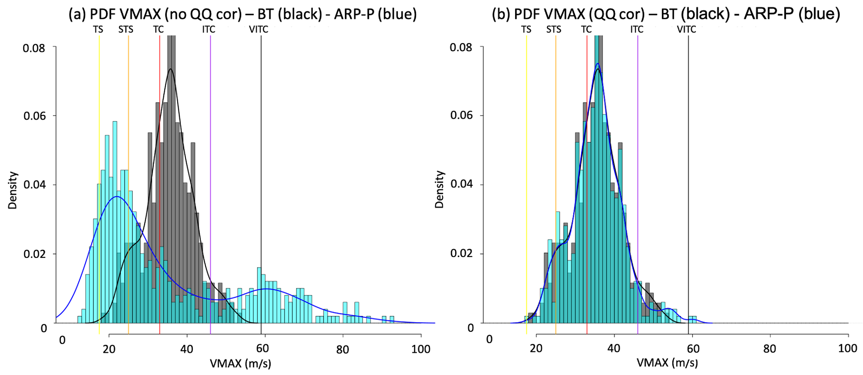
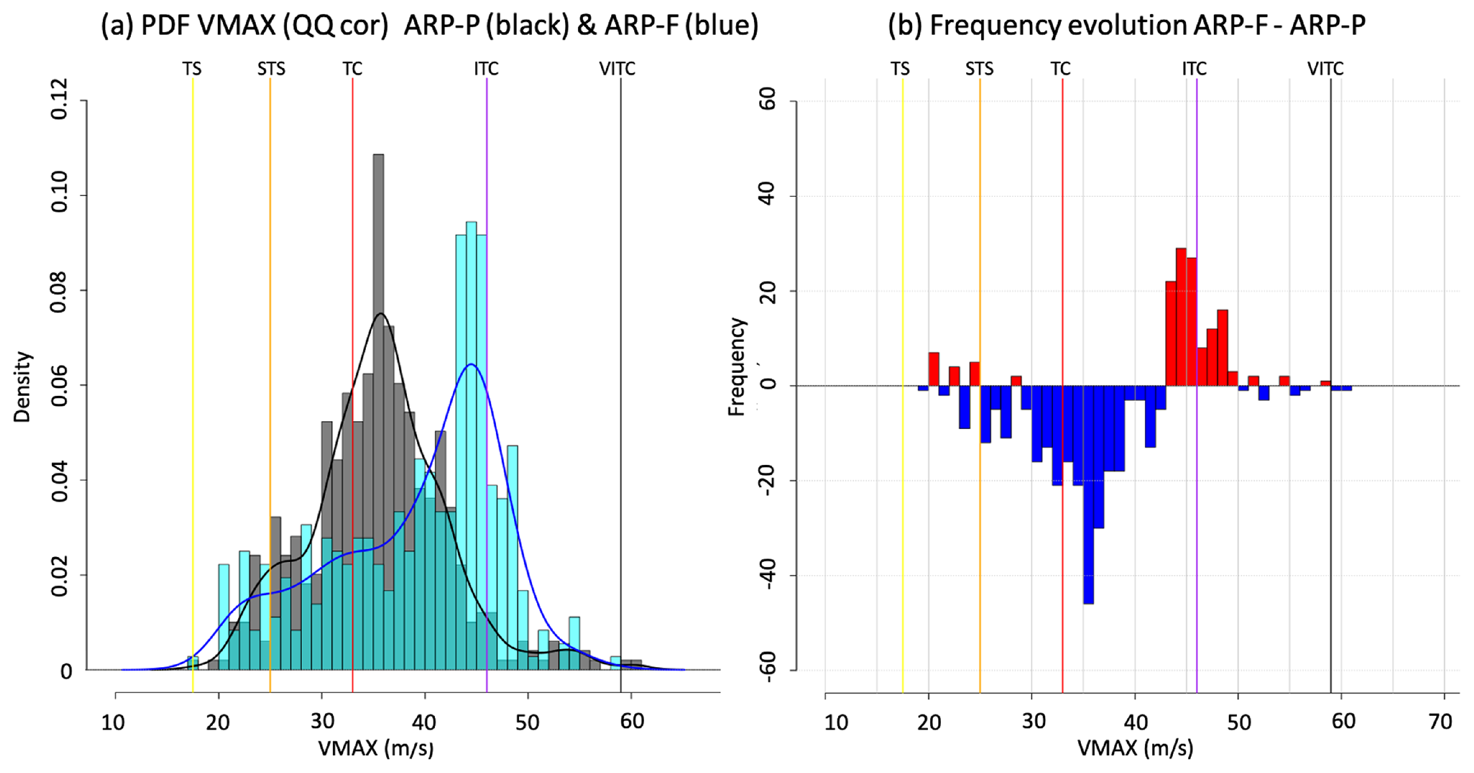
4.2. Simulated Frequency and Intensity of Future TC

After applying a QQ correction to both present- and future-day simulations, one can therefore estimate potential changes in cyclonic activity between the two simulated epochs with respect to “real world” TC classifications. Figure 11a shows the PDF of the $V_{MAX}$ for tracked CS simulated in ARP-F (blue) and ARP-P (grey) simulations, classified by storm intensity category. Through considering all intensity classes, one can note an average frequency decrease of nearly 20–25% between ARP-P and ARP-F simulations. This result is consistent with the previous global analysis of Cattiaux et al. [13] that showed a reduction of the cyclonic season length of about 1 month (20%) between the two simulated epochs. Going into the details, one can notice an overall decrease of the storm intensities for TS and TC categories between the two epochs but also a significant increase for higher intensity systems. The changes in storm frequency (days of cyclonic activity) shown in Figure 11b indicate that the largest decrease in frequency occurs for low-to-moderate intensity systems ($V_{MAX}$ < 42 m s${}^{-1}$). On average, the number of days of cyclonic activity between the two epochs is (i) significantly reduced for TSs (MTS, STS) and lower intensity TCs (TC-, 33 < $V_{MAX}$ < 42 m s${}^{-1}$), which all together represent ∼75% of CS developing in the basin, (ii) significantly increased for higher intensity TC (TC+) and lower intensity ITC (ITC-) systems (42 < $V_{MAX}$ < 50 m s${}^{-1}$), and (iii) globally unchanged for the most intense storms ($V_{MAX}$ > 50 m s${}^{-1}$).

Figure 12a also suggests that storm intensities should be subject to significant changes in the future (plain red line) with respect to present time (plain black line). Hence, one can note an overall decrease of the intensity for all TS with $V_{MAX}$ < 25 m s${}^{-1}$, an increase for all storms with $V_{MAX}$ between 25 m s${}^{-1}$ and 50 m s${}^{-1}$ (i.e., STS, TC, and ITC-), and almost no change for the most intense systems ($V_{MAX}$ > 50 m s${}^{-1}$, ITC+ and VITC). Due to the small sample size for the latter categories, these numbers should however be taken cautiously. Expressing these differences as percentages for each storm category gives a decrease of up to ∼2 m s${}^{-1}$ (∼10%) for MTS and increases of up to ∼1.8 m s${}^{-1}$ (∼5%) for STS, 7.5 m s${}^{-1}$ (∼20%) for TC, and 6 m s${}^{-1}$ (∼14%) for ITC- (42 < $V_{MAX}$ < 50 m s${}^{-1}$). The mean position of the storm LMI, as derived from best-track and model simulations, is also shown in Figure 12b. In the present-time simulation (blue), one can note that the mean latitude of the LMI is shifted southward by ∼0.5${}^{\circ }$ with respect to best-track data (white) and that the dispersion is also larger in the model. This confirms the slight tendency of CNRM-CM to slightly overestimate TC intensification in the southern part of the basin, which was already noticed by Cattiaux et al. [13]. Though comparing the mean latitudes of the LMI in ARP-P (blue) and ARP-F (grey) simulations, one can notice that the location of this maximum is shifted southwards by ∼1.5${}^{\circ }$ (i.e., to ∼22${}^{\circ }$ S) in the future (in good agreement with the previous study of Kossin et al. [107]).

All together, these results provide unprecedented detailed projections of TC activity in the SWIO in the second half of the century and suggest that all storm categories should be impacted differently by climate change:

• MTS should be slightly more frequent, but less intense;
• STS should become less frequent, but more intense;
• Low intensity TC (TC-, 33 < $V_{MAX}$ < 42 m s${}^{-1}$) should be less frequent, but significantly more intense;
• High intensity TC and low intensity ITC (TC+ and ITC-, 42 < $V_{MAX}$ < 50 m s${}^{-1}$) should be more frequent and more intense;
• ITC+ and VITC ($V_{MAX}$ > 50 m s${}^{-1}$) should not experience significant changes.

Because Réunion and Mauritius islands are essentially concerned by STS and TC, these results also suggest that the cyclonic activity during the second half of the century should be significantly enhanced in the Mascarene Archipelago. Thus, despite an overall decrease in frequency of these two storm categories, their increased intensity, which could reach up to 20% for TCs, combined with the migration of the storm LMI near 22${}^{\circ }$ S (which more of less corresponds to the latitude of Réunion and Mauritius islands), could lead to a significant increase of TC-related hazards in these two territories. These results, only based on two simulations, are obviously to be taken with precaution and will have to be confirmed by the analysis of other high-resolution regional or global simulations. In this regard, the use of high-resolution model runs made in the frame of CMIP6 and BRIO (https://www.commissionoceanindien.org/portfolio-items/brio/, accessed on 27 May 2021) should allow one to further evaluate the realism of this scenario (work in progress). Future research work will also focus on the analysis of the differences in large scale environments to investigate possible relationships between the evolution of the atmospheric parameters (wind shear, moisture, vorticity...) and observed changes in TC activity.

In addition, in the frame of RNR-CYC, Thompson et al. [67] used a pseudo global warming method to estimate the projected change of a Bejisa-like TC in the second half of the century with a projected SST warming of 1.1–4.2 ${}^{\circ }$C (RCP 8.5 scenario). Such a TC has the potential to be more intense (+6.5% on average), to reach its LMI 2${}^{\circ }$ further poleward, and with a 33.8% increase of the median rainrate. This preliminary study enabled the building of an initialization and modeling approach that can now be used on several systems, with different climate perturbations. Such complementary km-scale resolution simulations [67] performed with the OWA coupled platform described in Section 2 should be conducted to further document the risk evolution on the inhabited islands of the basin.

5. Conclusions

The RNR-CYC programme consisted of two parts: the development of an observation network in the SWIO [15] conducted in close synergy with the implementation of numerical tools to model and analyze tropical cyclones behavior and impacts in the present and in a context of climate change. The modeling part which was the subject of this paper aimed at developing a unique coupled system to simulate TCs in the SWIO. Not only was the OWA coupling addressed but also a coherent coupling between sea state, wind field, aerosol, microphysics, and radiation was considered. Several cases of TCs that developed in the SWIO were modeled with the full scheme or part of it and evaluated against conventional or original observations like sea-turtles borne measurements [15,39]. These TCs simulations aimed at producing high resolution maps of wind, precipitation, and significant wave height to feed the three other subprograms of ReNovRisk [14]. These model outputs will be made available to the community as open access through the Geosur database development [14] (https://geosur.univ-reunion.fr/web/, accessed on 27 May 2021). These TCs simulations have also underlined several important results. In addition to the need for a 3D ocean–atmosphere coupling to correctly describe the intensity and the structure of ocean surface cooling in the wake of the TC [66], the significant role of sea salt aerosols (as the main source of CCN in TCs) in representing the track, intensity, and structure of TCs has been underlined [33]. The importance of coupling the ocean–atmosphere system with a wave model has also been highlighted to produce sea state coherent with the atmospheric and oceanic fields, which is crucial for sea salt aerosol emission [23] and for certain air–sea flux parameterizations. While further validation is still needed, the simulation of TC Idai presented herein perfectly illustrates the interconnections between the different models and parameterizations. It is the first attempt to simulate a TC with such a high degree of coupling, i.e., coupling between ocean, atmosphere, and wave models associated with an advanced and comprehensive coupling between aerosol, microphysics, and radiation parameterizations. Finally, the AROME/NEMO simulations of TC Herold allowed for the assessment for the first time of the performance of the future coupled TC model to be eventually used by RSMC La Réunion in the SWIO, as well as to evaluate the added value of the observations collected during RNR-CYC to assess more precisely the performance of the oceanic and atmospheric components of this coupled system under cyclonic conditions. Sea turtle borne observations, which will soon be extended to the Mozambique Channel and north-western part of the SWIO basin, appear as a very exciting means to complement oceanic satellite observations and rare in-situ measurements available in the SWIO to evaluate ocean model forecasts within and underneath the OML.

The climate component of RNR-CYC also provided unique climate simulations to assess the evolution of TC activity in the SWIO during the second half of the 21st century and helped in implementing new approaches to accurately estimate the evolution, in terms of intensity and frequency, of the different categories of low-pressure tropical systems in this area. At both ends of the spectrum, it appears that TSs should become less frequent and slightly more intense in the future, while the most intense systems ($V_{MAX}$ > 50 m s${}^{-1}$) should not experience significant changes. Changes, however, appear significantly more important for intermediate intensity systems such as TC and ITC (33 m s${}^{-1}$ < $V_{MAX}$ < 50 m s${}^{-1}$), whose intensity increase could reach up to 20% in the future. Overall, these results suggest that the Mascarene Archipelago, and in particular Réunion and Mauritius islands, should experience a significant increase of TC-related hazards in the medium term. The OWA coupled system developed in the frame of RNR-CYC can be used as a complementary tool of climate model analysis. For example, Thompson et al. [67] used this coupled system to simulate how the characteristics of TC Bejisa could change in response to global warming. This initialization and modeling procedure could be used to simulate a large series of systems for different emission scenarios to analyze the projected impact of tropical storms on the SWIO territories.

The validation of the mesoscale modeling platform will continue based on observations from RNR-CYC [15], new research programs such as the extension of the sea-turtle observing program initiated in RNR-CYC that will allow collecting in-situ ocean data throughout the entire Indian Ocean, and satellite observations, with a multiplication of simulations of TCs with different characteristics in terms of track, intensity, development region, structure, translation speed... Systematic comparisons of ocean, wave and atmosphere model outputs with available observations (e.g., analysis of the seismic noise for swell properties retrieval, temperature and salinity profiles in the upper layer of the ocean from gliders, Global Navigation Satellite System measurements for the integrated water vapor, etc.) on a large number of systems would enable one to propose an optimal configuration of the OWA platform for TC forecasting. As shown in Duong et al. [91], SAR data obtained during RNR-CYC have started being implemented in the 3D-Var assimilation scheme of AROME in its research version. Since AROME analysis can be used as initial and lateral boundary conditions for Meso-NH, improved AROME analysis would also be a benefit to the OWA coupled simulations involving Meso-NH through a better position, intensity, and structure of the vortex in the initial state.

Several improvements are already planned concerning ice microphysics and sea sprays. A key issue concerns the role of sea sprays in air–sea flux and in cloud microphysics and more particularly the sea spray emission function in extreme conditions. We will rely on Boreal unmanned airborne system flights in the environment of TC Joaninha (2019) [15]. Measurements of aerosol concentration, wind, wave height and sea state, SST, and meteorological parameters will enable a better evaluation and calibration of the sea salt aerosol flux. Moreover, new observations in ocean–atmosphere interactions in strong winds and high waves conditions will arise from the Marion Dufresne Atmospheric program (MAP-IO; http://www.mapio.re/, accessed on 27 May 2021) during which numerous instruments loaded onboard the Marion Dufresne vessel will collect data along its routes in the Indian and Southern oceans.

References

1. Neumann, C. Global Guide to Tropical Cyclone Forecasting, WMO Trop. Cyclone Program Rep. TCP-31; World Meteorological Organization: Geneva, Switzerland, 1993; p. 43. [Google Scholar]
2. WMO. Global Guide to Tropical Cyclone Forecasting; WMO: Geneva, Switzerland, 2017. [Google Scholar]
3. Leroux, M.D.; Meister, J.; Mékiès, D.; Dorla, A.L.; Caroff, P. A Climatology of Southwest Indian Ocean Tropical Systems: Their Number, Tracks, Impacts, Sizes, Empirical Maximum Potential Intensity, and Intensity Changes. J. Appl. Meteorol. Climatol. 2018, 57, 1021–1041. [Google Scholar] [CrossRef]
4. Quetelard, H.; Bessemoulin, P.; Cerveny, R.S.; Peterson, T.C.; Burton, A.; Boodhoo, Y. Extreme Weather: World-Record Rainfalls During Tropical Cyclone Gamede. Bull. Am. Meteorol. Soc. 2009, 90, 603–608. [Google Scholar] [CrossRef]
5. Leroux, M.D.; Wood, K.; Elsberry, R.L.; Cayanan, E.O.; Hendricks, E.; Kucas, M.; Otto, P.; Rogers, R.; Sampson, B.; Yu, Z. Recent Advances in Research and Forecasting of Tropical Cyclone Track, Intensity, and Structure at Landfall. Trop. Cyclone Res. Rev. 2018, 7, 85–105. [Google Scholar] [CrossRef]
6. Chauvin, F.; Royer, J.F.; Déqué, M. Response of hurricane-type vortices to global warming as simulated by ARPEGE-Climat at high resolution. Clim. Dyn. 2006, 27, 377–399. [Google Scholar] [CrossRef]
7. Knutson, T.R.; McBride, J.L.; Chan, J.; Emanuel, K.; Holland, G.; Landsea, C.; Held, I.; Kossin, J.P.; Srivastava, A.K.; Sugi, M. Tropical cyclones and climate change. Nat. Geosci. 2010, 3, 157–163. [Google Scholar] [CrossRef] [Green Version]
8. Sugi, M.; Murakami, H.; Yoshimura, J. On the Mechanism of Tropical Cyclone Frequency Changes Due to Global Warming. J. Meteorol. Soc. Jpn. Ser. II 2012, 90A, 397–408. [Google Scholar] [CrossRef] [Green Version]
9. Christensen, J.; Krishna Kumar, K.; Aldrian, E.; An, S.I.; Cavalcanti, I.; de Castro, M.; Dong, W.; Goswami, P.; Hall, A.; Kanyanga, J.; et al. Climate Phenomena and their Relevance for Future Regional Climate Change; Technical Report; Cambridge University Press: Cambridge, UK, 2014. [Google Scholar] [CrossRef]
10. Knutson, T.R.; Sirutis, J.J.; Zhao, M.; Tuleya, R.E.; Bender, M.; Vecchi, G.A.; Villarini, G.; Chavas, D. Global Projections of Intense Tropical Cyclone Activity for the Late Twenty-First Century from Dynamical Downscaling of CMIP5/RCP4.5 Scenarios. J. Clim. 2015, 28, 7203–7224. [Google Scholar] [CrossRef] [Green Version]
11. Knutson, T.; Camargo, S.J.; Chan, J.C.L.; Emanuel, K.; Ho, C.H.; Kossin, J.; Mohapatra, M.; Satoh, M.; Sugi, M.; Walsh, K.; et al. Tropical Cyclones and Climate Change Assessment: Part II: Projected Response to Anthropogenic Warming. Bull. Am. Meteorol. Soc. 2020, 101, E303–E322. [Google Scholar] [CrossRef]
12. Walsh, K.J.E.; McBride, J.L.; Klotzbach, P.J.; Balachandran, S.; Camargo, S.J.; Holland, G.; Knutson, T.R.; Kossin, J.P.; Lee, T.C.; Sobel, A.; et al. Tropical cyclones and climate change. WIREs Clim. Chang. 2016, 7, 65–89. [Google Scholar] [CrossRef]
13. Cattiaux, J.; Chauvin, F.; Bousquet, O.; Malardel, S.; Tsai, C.L. Projected Changes in the Southern Indian Ocean Cyclone Activity Assessed from High-Resolution Experiments and CMIP5 Models. J. Clim. 2020, 33, 4975–4991. [Google Scholar] [CrossRef] [Green Version]
14. Tulet, P.; Aunay, B.; Barruol, G.; Barthe, C.; Belon, R.; Bielli, S.; Bonnardot, F.; Bousquet, O.; Cammas, J.P.; Cattiaux, J.; et al. ReNovRisk: A multidisciplinary programme to study the cyclonic risks in the South-West Indian Ocean. Nat. Hazards 2021, 107, 1191–1223. [Google Scholar] [CrossRef]
15. Bousquet, O.; Barruol, G.; Cordier, E.; Barthe, C.; Bielli, S.; Tulet, P.; Amelie, V.; Fletcher-Dogley, F.; Mavume, A.; Zucule, J.; et al. Impact of tropical cyclones on inhabited areas of the SWIO basin at present and future horizons. Part 1: Overview and observing component of the research program RENOVRISK-CYCLONE. Atmosphere 2021, 12, 544. [Google Scholar] [CrossRef]
16. Bender, M.A.; Ginis, I. Real-Case Simulations of Hurricane–Ocean Interaction Using A High-Resolution Coupled Model: Effects on Hurricane Intensity. Mon. Weather Rev. 2000, 128, 917–946. [Google Scholar] [CrossRef]
17. Sandery, P.A.; Brassington, G.B.; Craig, A.; Pugh, T. Impacts of Ocean–Atmosphere Coupling on Tropical Cyclone Intensity Change and Ocean Prediction in the Australian Region. Mon. Weather Rev. 2010, 138, 2074–2091. [Google Scholar] [CrossRef]
18. Lee, C.Y.; Chen, S.S. Stable Boundary Layer and Its Impact on Tropical Cyclone Structure in a Coupled Atmosphere–Ocean Model. Mon. Weather Rev. 2014, 142, 1927–1944. [Google Scholar] [CrossRef]
19. Mogensen, K.S.; Magnusson, L.; Bidlot, J.R. Tropical cyclone sensitivity to ocean coupling in the ECMWF coupled model. J. Geophys. Res. Ocean. 2017, 122, 4392–4412. [Google Scholar] [CrossRef]
20. Warner, J.C.; Armstrong, B.; He, R.; Zambon, J.B. Development of a Coupled Ocean–Atmosphere–Wave–Sediment Transport (COAWST) Modeling System. Ocean Model. 2010, 35, 230–244. [Google Scholar] [CrossRef] [Green Version]
21. Liu, B.; Liu, H.; Xie, L.; Guan, C.; Zhao, D. A Coupled Atmosphere–Wave–Ocean Modeling System: Simulation of the Intensity of an Idealized Tropical Cyclone. Mon. Weather Rev. 2011, 139, 132–152. [Google Scholar] [CrossRef]
22. Chen, S.S.; Zhao, W.; Donelan, M.A.; Tolman, H.L. Directional Wind–Wave Coupling in Fully Coupled Atmosphere–Wave–Ocean Models: Results from CBLAST-Hurricane. J. Atmos. Sci. 2013, 70, 3198–3215. [Google Scholar] [CrossRef]
23. Pianezze, J.; Barthe, C.; Bielli, S.; Tulet, P.; Jullien, S.; Cambon, G.; Bousquet, O.; Claeys, M.; Cordier, E. A New Coupled Ocean-Waves-Atmosphere Model Designed for Tropical Storm Studies: Example of Tropical Cyclone Bejisa (2013–2014) in the South-West Indian Ocean. J. Adv. Model. Earth Syst. 2018, 10, 801–825. [Google Scholar] [CrossRef] [Green Version]
24. Aijaz, S.; Ghantous, M.; Babanin, A.V.; Ginis, I.; Thomas, B.; Wake, G. Nonbreaking wave-induced mixing in upper ocean during tropical cyclones using coupled hurricane-ocean-wave modeling. J. Geophys. Res. Ocean. 2017, 122, 3939–3963. [Google Scholar] [CrossRef] [Green Version]
25. Andreas, E.L. The Temperature of Evaporating Sea Spray Droplets. J. Atmos. Sci. 1995, 52, 852–862. [Google Scholar] [CrossRef] [Green Version]
26. Andreas, E.L. Sea spray and the turbulent air-sea heat fluxes. J. Geophys. Res. Ocean. 1992, 97, 11429–11441. [Google Scholar] [CrossRef]
27. Wang, Y.; Kepert, J.D.; Holland, G.J. The Effect of Sea Spray Evaporation on Tropical Cyclone Boundary Layer Structure and Intensity. Mon. Weather Rev. 2001, 129, 2481–2500. [Google Scholar] [CrossRef] [Green Version]
28. Bao, J.W.; Fairall, C.W.; Michelson, S.A.; Bianco, L. Parameterizations of Sea-Spray Impact on the Air–Sea Momentum and Heat Fluxes. Mon. Weather Rev. 2011, 139, 3781–3797. [Google Scholar] [CrossRef]
29. Emanuel, K. 100 Years of Progress in Tropical Cyclone Research. Meteorol. Monogr. 2018, 59, 15.1–15.68. [Google Scholar] [CrossRef]
30. Andreae, M.; Rosenfeld, D. Aerosol–cloud–precipitation interactions. Part 1. The nature and sources of cloud-active aerosols. Earth-Sci. Rev. 2008, 89, 13–41. [Google Scholar] [CrossRef]
31. Rosenfeld, D.; Woodley, W.L.; Khain, A.; Cotton, W.R.; Carrió, G.; Ginis, I.; Golden, J.H. Aerosol Effects on Microstructure and Intensity of Tropical Cyclones. Bull. Am. Meteorol. Soc. 2012, 93, 987–1001. [Google Scholar] [CrossRef]
32. Shpund, J.; Khain, A.; Rosenfeld, D. Effects of Sea Spray on Microphysics and Intensity of Deep Convective Clouds Under Strong Winds. J. Geophys. Res. Atmos. 2019, 124, 9484–9509. [Google Scholar] [CrossRef]
33. Hoarau, T.; Barthe, C.; Tulet, P.; Claeys, M.; Pinty, J.P.; Bousquet, O.; Delanoë, J.; Vié, B. Impact of the Generation and Activation of Sea Salt Aerosols on the Evolution of Tropical Cyclone Dumile. J. Geophys. Res. Atmos. 2018, 123, 8813–8831. [Google Scholar] [CrossRef]
34. Trabing, B.C.; Bell, M.M.; Brown, B.R. Impacts of Radiation and Upper-Tropospheric Temperatures on Tropical Cyclone Structure and Intensity. J. Atmos. Sci. 2019, 76, 135–153. [Google Scholar] [CrossRef]
35. Ruppert, J.H.; Wing, A.A.; Tang, X.; Duran, E.L. The critical role of cloud-infrared radiation feedback in tropical cyclone development. Proc. Natl. Acad. Sci. USA 2020, 117, 27884–27892. [Google Scholar] [CrossRef]
36. Zadra, A.; Williams, K.; Frassoni, A.; Rixen, M.; Adames, A.F.; Berner, J.; Bouyssel, F.; Casati, B.; Christensen, H.; Ek, M.B.; et al. Systematic Errors in Weather and Climate Models: Nature, Origins, and Ways Forward. Bull. Am. Meteorol. Soc. 2018, 99, ES67–ES70. [Google Scholar] [CrossRef] [Green Version]
37. Lac, C.; Chaboureau, J.P.; Masson, V.; Pinty, J.P.; Tulet, P.; Escobar, J.; Leriche, M.; Barthe, C.; Aouizerats, B.; Augros, C.; et al. Overview of the Meso-NH model version 5.4 and its applications. Geosci. Model Dev. 2018, 11, 1929–1969. [Google Scholar] [CrossRef] [Green Version]
38. Seity, Y.; Brousseau, P.; Malardel, S.; Hello, G.; Bénard, P.; Bouttier, F.; Lac, C.; Masson, V. The AROME-France Convective-Scale Operational Model. Mon. Weather Rev. 2011, 139, 976–991. [Google Scholar] [CrossRef] [Green Version]
39. Bousquet, O.; Dalleau, M.; Bocquet, M.; Gaspar, P.; Bielli, S.; Ciccione, S.; Remy, E.; Vidard, A. Sea Turtles for Ocean Research and Monitoring: Overview and Initial Results of the STORM Project in the Southwest Indian Ocean. Front. Mar. Sci. 2020, 7, 859. [Google Scholar] [CrossRef]
40. Radnoti, G.; Ajjaji, R.; Bubnova, R.; Caian, M.; Cordoneanu, E.; Emde, K.; Grill, J.D.; Hoffman, J.; Horanyi, A.; Issara, S.; et al. The spectral limited area model ARPEGE/ALADIN. PWRP Rep. Ser. 1995, 7, 111–117. [Google Scholar]
41. Lebeaupin Brossier, C.; Ducrocq, V.; Giordani, H. Two-way one-dimensional high-resolution air–sea coupled modelling applied to Mediterranean heavy rain events. Q. J. R. Meteorol. Soc. 2009, 135, 187–204. [Google Scholar] [CrossRef]
42. Bloom, S.C.; Takacs, L.L.; da Silva, A.M.; Ledvina, D. Data Assimilation Using Incremental Analysis Updates. Mon. Weather Rev. 1996, 124, 1256–1271. [Google Scholar] [CrossRef] [Green Version]
43. Masson, V.; Le Moigne, P.; Martin, E.; Faroux, S.; Alias, A.; Alkama, R.; Belamari, S.; Barbu, A.; Boone, A.; Bouyssel, F.; et al. The SURFEXv7.2 land and ocean surface platform for coupled or offline simulation of earth surface variables and fluxes. Geosci. Model Dev. 2013, 6, 929–960. [Google Scholar] [CrossRef] [Green Version]
44. Noilhan, J.; Planton, S. A Simple Parameterization of Land Surface Processes for Meteorological Models. Mon. Wea. Rev. 1989, 117, 536–549. [Google Scholar] [CrossRef]
45. Masson, V. A Physically-Based Scheme For The Urban Energy Budget in Atmospheric Models. Bound.-Layer Meteorol. 2000, 94, 357–397. [Google Scholar] [CrossRef]
46. Mironov, D.; Heise, E.; Kourzeneva, E.; Ritter, B.; Schneider, N.; Terzhevik, A. Implementation of the lake parameterisation scheme FLake into the numerical weather prediction model COSMO. Boreal Environ. Res. 2010, 15, 218–230. [Google Scholar]
47. Fairall, C.W.; Bradley, E.F.; Hare, J.E.; Grachev, A.A.; Edson, J.B. Bulk Parameterization of Air–Sea Fluxes: Updates and Verification for the COARE Algorithm. J. Clim. 2003, 16, 571–591. [Google Scholar] [CrossRef]
48. Belamari, S. Report on uncertainty estimates of an optimal bulk formulation for surface turbulent fluxes. Marine EnviRonment and Security for the European Area—Integrated Project (MERSEA IP) Deliverable D.4.1.2, 2005. [Google Scholar]
49. Gaspar, P.; Grégoris, Y.; Lefevre, J.M. A simple eddy kinetic energy model for simulations of the oceanic vertical mixing: Tests at station Papa and long-term upper ocean study site. J. Geophys. Res. Ocean. 1990, 95, 16179–16193. [Google Scholar] [CrossRef]
50. Voldoire, A.; Decharme, B.; Pianezze, J.; Lebeaupin Brossier, C.; Sevault, F.; Seyfried, L.; Garnier, V.; Bielli, S.; Valcke, S.; Alias, A.; et al. SURFEX v8.0 interface with OASIS3-MCT to couple atmosphere with hydrology, ocean, waves and sea-ice models, from coastal \hack\newlineto global scales. Geosci. Model Dev. 2017, 10, 4207–4227. [Google Scholar] [CrossRef] [Green Version]
51. Madec, G.; Bourdallé-Badie, R.; Chanut, J.; Emanuela Clementi, E.; Coward, A.; Ethé, C.; Iovino, D.; Lea, D.; Lévy, C.; Lovato, T.; et al. NEMO Ocean Engine. 2019. Available online: https://zenodo.org/record/3878122#.YLBaZaERWUk (accessed on 27 May 2021). [CrossRef]
52. Shchepetkin, A.F.; McWilliams, J.C. The regional oceanic modeling system (ROMS): A split-explicit, free-surface, topography-following-coordinate oceanic model. Ocean Model. 2005, 9, 347–404. [Google Scholar] [CrossRef]
53. Debreu, L.; Marchesiello, P.; Penven, P.; Cambon, G. Two-way nesting in split-explicit ocean models: Algorithms, implementation and validation. Ocean Model. 2012, 49–50, 1–21. [Google Scholar] [CrossRef]
54. Klein, P.; Hua, B.L.; Lapeyre, G.; Capet, X.; Gentil, S.L.; Sasaki, H. Upper Ocean Turbulence from High-Resolution 3D Simulations. J. Phys. Oceanogr. 2008, 38, 1748–1763. [Google Scholar] [CrossRef] [Green Version]
55. Tolman, H.L.; Chalikov, D. Source Terms in a Third-Generation Wind Wave Model. J. Phys. Oceanogr. 1996, 26, 2497–2518. [Google Scholar] [CrossRef] [Green Version]
56. Craig, A.; Valcke, S.; Coquart, L. Development and performance of a new version of the OASIS coupler, OASIS3-MCT_3.0. Geosci. Model Dev. 2017, 10, 3297–3308. [Google Scholar] [CrossRef] [Green Version]
57. Couvelard, X.; Lemarié, F.; Samson, G.; Redelsperger, J.L.; Ardhuin, F.; Benshila, R.; Madec, G. Development of a two-way-coupled ocean–wave model: Assessment on a global NEMO(v3.6)–WW3(v6.02) coupled configuration. Geosci. Model Dev. 2020, 13, 3067–3090. [Google Scholar] [CrossRef]
58. Ovadnevaite, J.; Manders, A.; de Leeuw, G.; Ceburnis, D.; Monahan, C.; Partanen, A.I.; Korhonen, H.; O’Dowd, C.D. A sea spray aerosol flux parameterization encapsulating wave state. Atmos. Chem. Phys. 2014, 14, 1837–1852. [Google Scholar] [CrossRef] [Green Version]
59. Tulet, P.; Crassier, V.; Cousin, F.; Suhre, K.; Rosset, R. ORILAM, a three-moment lognormal aerosol scheme for mesoscale atmospheric model: Online coupling into the Meso-NH-C model and validation on the Escompte campaign. J. Geophys. Res. Atmos. 2005, 110. [Google Scholar] [CrossRef]
60. Tulet, P.; Crahan-Kaku, K.; Leriche, M.; Aouizerats, B.; Crumeyrolle, S. Mixing of dust aerosols into a mesoscale convective system: Generation, filtering and possible feedbacks on ice anvils. Atmos. Res. 2010, 96, 302–314. [Google Scholar] [CrossRef] [Green Version]
61. Vié, B.; Pinty, J.P.; Berthet, S.; Leriche, M. LIMA (v1.0): A quasi two-moment microphysical scheme driven by a multimodal population of cloud condensation and\hack\break ice freezing nuclei. Geosci. Model Dev. 2016, 9, 567–586. [Google Scholar] [CrossRef] [Green Version]
62. Chen, J.P.; Lamb, D. The Theoretical Basis for the Parameterization of Ice Crystal Habits: Growth by Vapor Deposition. J. Atmos. Sci. 1994, 51, 1206–1222. [Google Scholar] [CrossRef]
63. Bailey, M.P.; Hallett, J. A Comprehensive Habit Diagram for Atmospheric Ice Crystals: Confirmation from the Laboratory, AIRS II, and Other Field Studies. J. Atmos. Sci. 2009, 66, 2888–2899. [Google Scholar] [CrossRef] [Green Version]
64. Sauvage, C.; Lebeaupin Brossier, C.; Bouin, M.N.; Ducrocq, V. Characterization of the air–sea exchange mechanisms during a Mediterranean heavy precipitation event using realistic sea state modelling. Atmos. Chem. Phys. 2020, 20, 1675–1699. [Google Scholar] [CrossRef] [Green Version]
65. Pinty, J.P.; Jabouille, P. A mixed-phase cloud parameterization for use in mesoscale non hydrostatic model: Simulations of a squall line and of orographic precipitations. In Proceedings of the the Conference on Cloud Physics, Everett, WA, USA, 17–21 August 1998; pp. 217–220. [Google Scholar]
66. Bielli, S.; Barthe, C.; Bousquet, O.; Tulet, P.; Pianezze, J. The effect of atmosphere-ocean coupling on the structure and intensity of tropical cyclone Bejisa observed in the southwest Indian ocean. Atmosphere 2021, submitted. [Google Scholar]
67. Thompson, C.; Barthe, C.; Bielli, S.; Tulet, P.; Pianezze, J. Projected Characteristic Changes of a Typical Tropical Cyclone under Climate Change in the South West Indian Ocean. Atmosphere 2021, 12, 232. [Google Scholar] [CrossRef]
68. Cuxart, J.; Bougeault, P.; Redelsperger, J.L. A turbulence scheme allowing for mesoscale and large-eddy simulations. Q. J. R. Meteorol. Soc. 2000, 126, 1–30. [Google Scholar] [CrossRef]
69. Bougeault, P.; Lacarrere, P. Parameterization of Orography-Induced Turbulence in a Mesobeta–Scale Model. Mon. Weather Rev. 1989, 117, 1872–1890. [Google Scholar] [CrossRef]
70. Bechtold, P.; Bazile, E.; Guichard, F.; Mascart, P.; Richard, E. A mass-flux convection scheme for regional and global models. Q. J. R. Meteorol. Soc. 2001, 127, 869–886. [Google Scholar] [CrossRef]
71. Gregory, D.; Morcrette, J.J.; Jakob, C.; Beljaars, A.C.M.; Stockdale, T. Revision of convection, radiation and cloud schemes in the ECMWF integrated forecasting system. Q. J. R. Meteorol. Soc. 2000, 126, 1685–1710. [Google Scholar] [CrossRef]
72. Mlawer, E.J.; Taubman, S.J.; Brown, P.D.; Iacono, M.J.; Clough, S.A. Radiative transfer for inhomogeneous atmospheres: RRTM, a validated correlated-k model for the longwave. J. Geophys. Res. Atmos. 1997, 102, 16663–16682. [Google Scholar] [CrossRef] [Green Version]
73. Inness, A.; Ades, M.; Agustí-Panareda, A.; Barré, J.; Benedictow, A.; Blechschmidt, A.M.; Dominguez, J.J.; Engelen, R.; Eskes, H.; Flemming, J.; et al. The CAMS reanalysis of atmospheric composition. Atmos. Chem. Phys. 2019, 19, 3515–3556. [Google Scholar] [CrossRef] [Green Version]
74. Moon, I.J.; Ginis, I.; Hara, T.; Thomas, B. A Physics-Based Parameterization of Air–Sea Momentum Flux at High Wind Speeds and Its Impact on Hurricane Intensity Predictions. Mon. Weather Rev. 2007, 135, 2869–2878. [Google Scholar] [CrossRef] [Green Version]
75. Andreas, E.L.; Mahrt, L.; Vickers, D. An improved bulk air–sea surface flux algorithm, including spray-mediated transfer. Q. J. R. Meteorol. Soc. 2015, 141, 642–654. [Google Scholar] [CrossRef]
76. Tolman, H.L. Alleviating the Garden Sprinkler Effect in wind wave models. Ocean Model. 2002, 4, 269–289. [Google Scholar] [CrossRef]
77. Ardhuin, F.; Rogers, E.; Babanin, A.V.; Filipot, J.F.; Magne, R.; Roland, A.; van der Westhuysen, A.; Queffeulou, P.; Lefevre, J.M.; Aouf, L.; et al. Semiempirical Dissipation Source Functions for Ocean Waves. Part I: Definition, Calibration, and Validation. J. Phys. Oceanogr. 2010, 40, 1917–1941. [Google Scholar] [CrossRef] [Green Version]
78. Hasselmann, S.; Hasselmann, K.; Allender, J.H.; Barnett, T.P. Computations and Parameterizations of the Nonlinear Energy Transfer in a Gravity-Wave Specturm. Part II: Parameterizations of the Nonlinear Energy Transfer for Application in Wave Models. J. Phys. Oceanogr. 1985, 15, 1378–1391. [Google Scholar] [CrossRef] [Green Version]
79. Battjes, J.A.; Janssen, J.P.F.M. Energy Loss and Set-Up Due to Breaking of Random Waves. Coast. Eng. 1978, 569–587. [Google Scholar] [CrossRef] [Green Version]
80. Ardhuin, F.; O’Reilly, W.C.; Herbers, T.H.C.; Jessen, P.F. Swell Transformation across the Continental Shelf. Part I: Attenuation and Directional Broadening. J. Phys. Oceanogr. 2003, 33, 1921–1939. [Google Scholar] [CrossRef]
81. Shchepetkin, A.F.; McWilliams, J.C. Quasi-Monotone Advection Schemes Based on Explicit Locally Adaptive Dissipation. Mon. Weather Rev. 1998, 126, 1541–1580. [Google Scholar] [CrossRef]
82. Large, W.G.; McWilliams, J.C.; Doney, S.C. Oceanic vertical mixing: A review and a model with a nonlocal boundary layer parameterization. Rev. Geophys. 1994, 32, 363–403. [Google Scholar] [CrossRef] [Green Version]
83. Madec, G.; Delécluse, P.; Imbard, M.; Lévy, C. OPA 8.1 Ocean General Circulation Model reference manual. Note Pole Modélisation 1998, 11, 91. [Google Scholar]
84. Lellouche, J.M.; Greiner, E.; Le Galloudec, O.; Garric, G.; Regnier, C.; Drevillon, M.; Benkiran, M.; Testut, C.E.; Bourdalle-Badie, R.; Gasparin, F.; et al. Recent updates to the Copernicus Marine Service global ocean monitoring and forecasting real-time 1/12F high-resolution system. Ocean Sci. 2018, 14, 1093–1126. [Google Scholar] [CrossRef] [Green Version]
85. Fairall, C.W.; Bradley, E.F.; Rogers, D.P.; Edson, J.B.; Young, G.S. Bulk parameterization of air-sea fluxes for Tropical Ocean-Global Atmosphere Coupled-Ocean Atmosphere Response Experiment. J. Geophys. Res. Ocean. 1996, 101, 3747–3764. [Google Scholar] [CrossRef]
86. Webster, P.J.; Lukas, R. TOGA COARE: The Coupled Ocean–Atmosphere Response Experiment. Bull. Am. Meteorol. Soc. 1992, 73, 1377–1416. [Google Scholar] [CrossRef] [Green Version]
87. Oost, W.; Komen, G.; Jacobs, C.; Van Oort, C. New evidence for a relation between wind stress and wave age from measurements during ASGAMAGE. Bound.-Layer Meteorol. 2002, 103, 409–438. [Google Scholar] [CrossRef]
88. Powell, M.D.; Vickery, P.J.; Reinhold, T.A. Reduced drag coefficient for high wind speeds in tropical cyclones. Nature 2003, 422, 279–283. [Google Scholar] [CrossRef]
89. Green, B.W.; Zhang, F. Impacts of Air–Sea Flux Parameterizations on the Intensity and Structure of Tropical Cyclones. Mon. Weather Rev. 2013, 141, 2308–2324. [Google Scholar] [CrossRef] [Green Version]
90. Veron, F. Ocean Spray. Annu. Rev. Fluid Mech. 2015, 47, 507–538. [Google Scholar] [CrossRef]
91. Duong, Q.P.; Langlade, S.; Payan, C.; Husson, R.; Mouche, A.; Malardel, S. C-band SAR Winds for Tropical Cyclone monitoring and forecast in the South-West Indian Ocean. Atmosphere 2021, 12, 576. [Google Scholar] [CrossRef]
92. Willoughby, H.E.; Jin, H.L.; Lord, S.J.; Piotrowicz, J.M. Hurricane Structure and Evolution as Simulated by an Axisymmetric, Nonhydrostatic Numerical Model. J. Atmos. Sci. 1984, 41, 1169–1186. [Google Scholar] [CrossRef] [Green Version]
93. Zhu, S.; Guo, X.; Lu, G.; Guo, L. Ice Crystal Habits and Growth Processes in Stratiform Clouds with Embedded Convection Examined through Aircraft Observation in Northern China. J. Atmos. Sci. 2015, 72, 2011–2032. [Google Scholar] [CrossRef]
94. Bousquet, O.; Barbary, D.; Bielli, S.; Kebir, S.; Raynaud, L.; Malardel, S.; Faure, G. An evaluation of tropical cyclone forecast in the Southwest Indian Ocean basin with AROME-Indian Ocean convection-permitting numerical weather predicting system. Atmos. Sci. Lett. 2020, 21, e950. [Google Scholar] [CrossRef]
95. Trenberth, K.E.; Fasullo, J.; Smith, L. Trends and variability in column-integrated atmospheric water vapor. Clim. Dyn. 2005, 24, 741–758. [Google Scholar] [CrossRef]
96. Trenberth, K.E.; Smith, L.; Qian, T.; Dai, A.; Fasullo, J. Estimates of the Global Water Budget and Its Annual Cycle Using Observational and Model Data. J. Hydrometeorol. 2007, 8, 758–769. [Google Scholar] [CrossRef]
97. Allan, R.P.; Soden, B.J. Atmospheric Warming and the Amplification of Precipitation Extremes. Science 2008, 321, 1481–1484. [Google Scholar] [CrossRef] [Green Version]
98. Chou, C.; Neelin, J.D.; Chen, C.A.; Tu, J.Y. Evaluating the “Rich-Get-Richer” Mechanism in Tropical Precipitation Change under Global Warming. J. Clim. 2009, 22, 1982–2005. [Google Scholar] [CrossRef]
99. Bengtsson, L.; Botzet, M.; Esch, M. Will greenhouse gas-induced warming over the next 50 years lead to higher frequency and greater intensity of hurricanes? Tellus A 1996, 48, 57–73. [Google Scholar] [CrossRef] [Green Version]
100. Bengtsson, L.; Hodges, K.I.; Esch, M.; Keenlyside, N.; Kornblueh, L.; Luo, J.J.; Yamagata, T. How may tropical cyclones change in a warmer climate? Tellus A 2007, 59, 539–561. [Google Scholar] [CrossRef] [Green Version]
101. Sugi, M. Toward Improved Projection of the Future Tropical Cyclone Changes. In Indian Ocean Tropical Cyclones and Climate Change; Charabi, Y., Ed.; Springer: Dordrecht, The Netherlands, 2010; pp. 29–35. [Google Scholar] [CrossRef]
102. Emanuel, K.; Sundararajan, R.; Williams, J. Hurricanes and Global Warming: Results from Downscaling IPCC AR4 Simulations. Bull. Am. Meteorol. Soc. 2008, 89, 347–368. [Google Scholar] [CrossRef]
103. Emanuel, K. Tropical Cyclone Activity Downscaled from NOAA-CIRES Reanalysis, 1908–1958. J. Adv. Model. Earth Syst. 2010, 2. [Google Scholar] [CrossRef]
104. Taylor, K.E.; Stouffer, R.J.; Meehl, G.A. An Overview of CMIP5 and the Experiment Design. Bull. Am. Meteorol. Soc. 2012, 93, 485–498. [Google Scholar] [CrossRef] [Green Version]
105. Camargo, S.J.; Tippett, M.K.; Sobel, A.H.; Vecchi, G.A.; Zhao, M. Testing the Performance of Tropical Cyclone Genesis Indices in Future Climates Using the HiRAM Model. J. Clim. 2014, 27, 9171–9196. [Google Scholar] [CrossRef]
106. Chauvin, F.; Pilon, R.; Palany, P.; Belmadani, A. Future changes in Atlantic hurricanes with the rotated-stretched ARPEGE-Climat at very high resolution. Clim. Dyn. 2020, 54, 947–972. [Google Scholar] [CrossRef]
107. Kossin, J.P.; Emanuel, K.A.; Vecchi, G.A. The poleward migration of the location of tropical cyclone maximum intensity. Nature 2014, 509, 349–352. [Google Scholar] [CrossRef] [Green Version]
108. Holland, G.; Bruyère, C.L. Recent intense hurricane response to global climate change. Clim. Dyn. 2014, 42, 617–627. [Google Scholar] [CrossRef] [Green Version]
109. Voldoire, A.; Sanchez-Gomez, E.; Salas y Mélia, D.; Decharme, B.; Cassou, C.; Sénési, S.; Valcke, S.; Beau, I.; Alias, A.; Chevallier, M.; et al. The CNRM-CM5.1 global climate model: Description and basic evaluation. Clim. Dyn. 2013, 40, 2091–2121. [Google Scholar] [CrossRef] [Green Version]
110. Rayner, N.A.; Parker, D.E.; Horton, E.B.; Folland, C.K.; Alexander, L.V.; Rowell, D.P.; Kent, E.C.; Kaplan, A. Global analyses of sea surface temperature, sea ice, and night marine air temperature since the late nineteenth century. J. Geophys. Res. Atmos. 2003, 108. [Google Scholar] [CrossRef]
111. Voldoire, A.; Saint-Martin, D.; Sénési, S.; Decharme, B.; Alias, A.; Chevallier, M.; Colin, J.; Guérémy, J.F.; Michou, M.; Moine, M.P.; et al. Evaluation of CMIP6 DECK Experiments With CNRM-CM6-1. J. Adv. Model. Earth Syst. 2019, 11, 2177–2213. [Google Scholar] [CrossRef] [Green Version]
112. Daloz, A.S.; Chauvin, F.; Walsh, K.; Lavender, S.; Abbs, D.; Roux, F. The ability of general circulation models to simulate tropical cyclones and their precursors over the North Atlantic main development region. Clim. Dyn. 2012, 39, 1559–1576. [Google Scholar] [CrossRef]
Figure 1. Schematic diagram of the coupling systems in TC numerical modeling. The OWA coupling is shown in black while the coupling inside the atmosphere/surface model is shown with blue, red, and purple colors. Fields exchanged among the atmospheric, wave, and oceanic models are shown in italic black; they are exchanged at intervals defined by the user (typically ∼ 10 min). Fields exchanged among the atmospheric schemes are shown in italic blue and purple; they are exchanged at each time step. In the atmospheric/surface model, the purple color shows schemes, fields, and exchanges that are common to the AROME and Meso-NH models. The schemes, fields, and exchanges that are specific to the Meso-NH model are shown with blue color. The exchanges specific to the AROME model are shown with red color. Adapted from Tulet et al. [14].
Atmosphere 12 00689 g001
Figure 2. (a) Track and (b) intensity defined by the minimum sea level pressure (MSLP, hPa) of TC Fantala between 14 March 2016 00 UTC and 25 March 2016 00 UTC. The best-track is plotted with black lines and stars. The colored lines correspond to the different simulations summarized in Table 2.
Atmosphere 12 00689 g002
Figure 3. (a) Momentum flux (m 2 s 2 ), (b) drag coefficient, (c) latent heat flux (W m 2 ), and (d) sensible heat flux (W m 2 ) vs. 10-m wind speed (m s 1 ). These pairs of values are extracted at each grid point over the whole domain on 18 April at 00 UTC when TC Fantala is at its maximum intensity. The average (colored dot) and standard deviation (colored segments) of each parameter are plotted for each parameterization every 2.5 m s 1 .
Atmosphere 12 00689 g003
Figure 4. (a) Track and, (b) intensity defined by the MSLP (hPa) of TC Idai between 11 March 00 UTC and 15 March 00 UTC. The best-track and the Meso-NH/WW3/CROCO simulations are shown as black and cyan lines, respectively. The city of Beira is displayed with a red circle.
Atmosphere 12 00689 g004
Figure 5. Horizontal cross sections of Idai on 12 March 2019 at 18 UTC, simulated with the Meso-NH/WW3/CROCO OWA coupled system. (a) 10-m wind speed (m s 1 ; colors) and significant wave height H s (2, 4, 6, 8 and 10 m isolines), (b) total instantaneous net sea salt aerosol flux (μg m 2 s 1 ), (c) available (colors) and activated (1 and 10 cm 3 isolines) CCN, and (d) total ice thickness (mm; colors) and instantaneous precipitation (10 mm h 1 isoline). In c) only the contribution of sea salt particles (with dry diameter higher than 80 nm) to CCN is shown.
Atmosphere 12 00689 g005
Figure 6. Horizontal cross sections of TC Idai on 14 March 2019: (a) SAR surface wind speed (m s 1 ) at 16:05 UTC, (b) 10-m wind speed (m s 1 ; colors) at 14:00 UTC simulated with the OWA coupled system.
Atmosphere 12 00689 g006
Figure 7. (a) Track and (b) intensity defined by the MSLP (hPa) of TC Herold. The best-track and the AROME/NEMO simulations are shown as black and color lines, respectively. The positions of ST India are displayed as grey triangles.
Atmosphere 12 00689 g007
Figure 8. 10-m wind field (m s 1 ) below TC Herold on 16 March 2020 at 02 UTC, as inferred from AROME/NEMO simulations initialized on (a) 14 March at 12 UTC (HR2), (b) 15 March at 12 UTC (HR3), and (c) surface wind field (m s 1 ) inferred from SAR-derived data.
Atmosphere 12 00689 g008
Figure 9. Vertical profiles of ocean temperature ( C) valid at 15 UTC on (a) 13, (b) 14, (c) 15 and (d) 16 March 2020, as deduced from observations collected by ST India (black line) and from simulations HR1 (blue line), HR2 (red line) and HR3 (green line). Sea turtle data are aggregated over a 3-h period centered at 15 UTC.
Atmosphere 12 00689 g009
Figure 10. Probability density function (PDF) of the maximum wind speed ( V M A X , m s 1 ) for cyclogenetic storms ( V M A X ≥ 17 m s 1 ) in the SWIO, as derived from best-track (BT) (grey bars and black curve) and ARP-P simulation (cyan bars and blue curve) data (a) prior and (b) after the quantile-to-quantile (QQ) correction. Yellow, orange, red, purple, and black lines indicate TS, STS, TC, ITC, and VITC intensity threshold values, respectively. Note that V M A X values less than 17 m s 1 correspond to the intensity of the tracked storms prior to their cyclogenesis.
Atmosphere 12 00689 g010
Figure 11. (a) As in Figure 10 but for corrected ARP-P (grey bars and curve) and ARP-F (blue bars and curve) simulations. (b) Evolution of the frequency (days of cyclonic activity) of CS between the two simulated epochs as a function of V M A X . Yellow, orange, red, purple, and black vertical lines indicate TS, STS, TC, ITC, and VITC intensity threshold values, respectively.
Atmosphere 12 00689 g011
Figure 12. Mean evolution of the LMI of simulated CS ( V M A X > 17 m s 1 ) between the two epochs. (a) Percentile values as deduced from ARP-P (black) and ARP-F (red) simulations before (dashed) and after (plain) QQ correction. (b) Average latitude of storm LMI, as derived from best-track (white), ARP-P (blue), and ARP-F (grey) data. In (a) yellow, orange, red, purple, and black horizontal lines indicate MTS, STS, TC, ITC, and VITC intensity threshold values, respectively.
Atmosphere 12 00689 g012