Large Roll Vortices Exhibited by Post-Tropical Cyclone Sandy during Landfall

Abstract

Roll vortices are frequent features of a hurricane’s boundary layer, with kilometer or sub-kilometer horizontal scale. In this study, we found that large roll vortices with O (10 km) horizontal wavelength occurred over land in Post-Tropical Cyclone Sandy (2012) during landfall on New Jersey. Various characteristics of roll vortices were corroborated by analyses of Doppler radar observations, a 500 m resolution Weather Research and Forecasting (WRF) simulation, and an idealized roll vortex model. The roll vortices were always linear-shaped, and their wavelengths of 5–14 km were generally larger than any previously published for a tropical cyclone over land. Based on surface wind observations and simulated WRF surface wind fields, we found that roll vortices significantly increased the probability of hazardous winds and likely caused the observed patchiness of treefall during Sandy’s landfall.

1. Introduction

Hurricanes are the costliest natural disasters to affect coastal communities around the globe, causing substantial property and human life losses each year (https://coast.noaa.gov/states/fast-facts/weather-disasters.html, accessed on 1 February 2021). When a hurricane approaches land, the devastating wind often causes extensive structural damage. Interestingly, the wind-caused damage sometimes has a patchy distribution; some areas experience major destruction, whereas surrounding areas are lightly affected [1]. Roll vortices (rolls hereafter) in the hurricane boundary layer are suspected to be responsible for the patchy damage patterns [2]. These organized features consist of vertically overturning circulations, and they are elongated approximately in the hurricane’s tangential wind direction. When rolls are present, they modulate the strength of the surface wind, typically by ±30% in wind speed [3]. Total wind is enhanced in their downdraft regions and reduced in their updraft regions, providing a mechanism for the patchy wind damage under hurricanes. This vertical motion also transports momentum and enthalpy between the surface and the free atmosphere of a hurricane, which plays a key role in modulating hurricane intensity.

Rolls do occur in boundary layers beyond hurricanes; in fact, rolls were originally associated with airmass cloud bands [4,5,6,7]. Furthermore, rolls with different characteristics and driving mechanisms have since been identified and classified [8,9], with multiple types of rolls also identified and classified for hurricanes [10,11,12,13,14,15]. Large eddy simulations have been used to characterize rolls at finer granularity in recent years [16,17,18], and most recently, rolls have even been observed to be associated with high wind bands in extratropical cyclones [19]. Theoretical underpinning for roll formation has been developed by Mourad and Brown [20] and specifically for hurricane environments by Foster [21]. The focus of our work is confined to rolls that occur in hurricane boundary layers beyond their eyewall. The particular novelty of our work is that large rolls were observed over land in the boundary layer of a landfalling storm, Post-Tropical Cyclone Sandy, and the observations were corroborated with two independent types of numerical simulations.

Hurricane Sandy made landfall on New Jersey in 2012 as a post-tropical cyclone (TC) and caused devastating storm surge flooding, extended power outages due to massive treefall, and 72 direct deaths in the continental Unites States, with 20 of them caused by tree blowdown [22]. The patchy nature of extensive treefall was experienced throughout Sandy’s landfall region, from eastern Pennsylvania, across New Jersey, and into southeastern New York and southwestern Connecticut. A small sample of pre-Sandy and post-Sandy treefall patch images was gathered by the authors from Landsat imagery in New Jersey (Figure 1). The treefall patch shape was elongated in the direction of treefall, implying that narrow swaths of higher wind speed caused the treefall therein and lending to the hypothesis that rolls might have occurred. In this work, we present robust evidence of rolls during Sandy’s landfall based on three types of Doppler radar observations and corroborate it with archived output from a 500 m resolution Weather Research and Forecasting (WRF) simulation. The formation mechanism of rolls and their impact on hazardous surface winds are also examined.

2. Data and Model Simulation

2.1. Doppler Radar Observations

Doppler radar data [23] is from the WSR-88D radar station KDIX located at Fort Dix, NJ (marked by star in Figure 2). The center of Post-Tropical Cyclone Sandy traversed southern New Jersey in a west-northwestward direction about 50 km south of the radar site. Full volume radar scans were produced approximately every 6 min, with a minimum elevation angle of 0.5 degree. Both reflectivity and radial velocity data were used, for which range resolutions were 1 and 0.25 km, respectively, with an azimuth resolution of 1 degree for both. Doppler radar measures the motion of precipitation particles in the direction of the radar beam. Hereafter, we refer to the velocity observed by Doppler radar as radar radial velocity, which should be distinguished from the radial velocity of the post-tropical cyclone.

To better reveal roll-induced velocity perturbations, we obtained the residual velocity field using a method similar to Morrison et al. [24]. We considered the mean radar radial velocity as the first harmonic of a Fourier analysis applied to the total radar radial velocity. Radar residual velocity was then obtained by subtracting the first harmonic from the total radar radial velocity. The actual TC-scale wind was not expected to be horizontally uniform within the circular area covered by the conical radar scan. Therefore, the obtained residual velocity not only contained roll-induced velocity perturbations but also asymmetric TC-scale features. Nevertheless, roll-induced velocity perturbations were better revealed in the radar residual velocity field (Figure 3).

To characterize the vertical wind profile during landfall, Doppler radar velocity azimuth display (VAD) wind profile data for Fort Dix, NJ, were analyzed. The wind profiles were calculated by the WSR-88D VAD algorithm [25], which was analogous to that described above, where the mean radar radial velocity was calculated as the first harmonic of a Fourier analysis applied to the total radar radial velocity. The method, however, was applied to each height among a predetermined set of heights above ground. Each of these heights intersected at least one radar elevation angle scan cone at a particular radar range. The mean radar radial velocity was then computed for each range and elevation angle pair that matched the appropriate height above ground. The result was a profile of wind speed and direction data for each radar volume scan, typically recorded every 6 min.

The radar speed and direction data were subsequently converted to radial and tangential wind components relative to Sandy’s storm center and its translation vector. Storm center coordinates were specified using best track data from Blake et al. [22]. Because of the relatively coarse temporal resolution of the observed track (intervals were at most 6 h), storm center coordinates were calculated for every radar 6 min scan time by linear interpolation between best track storm center positions. The storm center translation vector was calculated for each best track storm center position as a mean vector among three track positions centered on a specified location. Analogous to the method used for storm center coordinates, translation vectors were also interpolated for each radar scan time. Finally, storm-centered cylindrical coordinates were used to compute the radial and tangential wind components relative to the translating storm center.

Since the profiles were calculated for the circular intersections of scan cones and height planes, they represent mean velocities for circles of various radii centered on the radar site at Fort Dix, NJ. The middle 50% of the distribution of these radii was in the range of 23–31 km, although the extremes reached 10 and 117 km.

2.2. WRF Simulation

Archived output from a 500 m resolution WRF simulation was used to corroborate the presence and characteristics of roll signatures observed by Doppler radar. Therefore, it was not possible to do any numerical experiments with the WRF simulation, nor modify any of the boundary or surface layer parametrizations to better represent an environment for rolls. Moreover, the fixed resolution of 500 m is known to be capable of manifesting rolls, yet not ideally and fully representing their characteristics, since the resolution resides in the “gray zone” of turbulence simulation [26,27,28], wherein the largest turbulent eddies are explicitly represented but smaller ones are parameterized. Nevertheless, signatures of rolls were exhibited by the WRF simulation whose characteristics agreed reasonably with those of rolls observed by radar. Therefore, we present the WRF-manifested roll signatures as corroborative evidence of roll presence in Sandy’s landfall but draw no significant conclusions from the WRF output because of the caveats described above.

The 96 h simulation was conducted using the Advanced Research WRF (version 3.3.1) initialized at 1200 UTC 26 October 2012 [29] using a horizontal resolution of 500 m. A single domain of size 2660 × 2500 km² (5320 × 5000 grid points) with 150 vertical layers (25 layers below 3 km height) was used without any nests. The time step was 1 s, and initial and boundary conditions were generated from the National Centers for Environmental Prediction Global Forecast System global model initialized at 1200 UTC 26 October 2012, with boundary conditions processed and applied every 6 forecast hours.

The Yonsei University (YSU) planetary boundary layer (PBL) scheme [30], the Noah land model [31], and the MM5 Monin–Obukhov similarity theory [32] surface layer model were used. Although the WRF physics was from a 2013 version, key physics for rolls is the PBL parameterization, which in our case was YSU, which is still being used for WRF simulations of small-scale vortices in TC PBLs for grid resolutions similar to that used herein (e.g., Wu et al. [33]). Cloud physics was modeled using WSM6 6-class microphysics with graupel [34]. Convection parameterization was not used for this high-resolution simulation. Three-hourly outputs of the dataset used herein are archived [35]. The 10 m surface winds diagnosed in WRF were strongly affected by surface roughness length over land, thus we chose to analyze winds at the lowest model layer (centered vertically at about 30 m height).

The WRF simulation closely represented Sandy’s observed landfall time (Figure 4), and the landfall location was only about 20 km south of the actual landfall location. This difference between the observed and simulated landfall location is small compared to (a) the distances between the analyzed roll signatures and the storm center and (b) the dimensions of areas populated by roll signatures, which are typically about 100 km. In addition, we did not use distance to the storm center as any quantitative characteristic of roll vortices. Furthermore, the roll analyses focused on radar observations, and the simulation data were used merely as corroborative evidence of roll presence. Therefore, the 20 km difference between observed and simulated landfall location should not have impacted any quantitative results presented herein.

Perturbation winds were obtained to reveal rolls’ impact on the surface wind distribution and their three-dimensional structure. We first horizontally smoothened the wind field using 100 passes of National Center for Atmospheric Research Command Language’s nine-point WRF two-dimensional field smoother to remove all roll-scale perturbations. Then, the perturbation fields were computed by subtracting the smoothed fields from the original. The obtained perturbations represented only flow features at the spatial scale of rolls or smaller.

2.3. Linearized Roll Vortex Model

The linearized roll model described in Gao and Ginis [36] was used to understand the formation mechanism of rolls exhibited in WRF. The linearized roll model resolves the most unstable normal mode under prescribed mean radial and tangential wind and virtual potential temperature profiles. The magnitude of roll velocities is assumed to be sufficiently small so that nonlinear advection terms are neglected. The rolls in the linear phase grow exponentially with time, but their basic structure remains unchanged. The actual velocity magnitude of the linear-phase rolls at any given time is not important. Therefore, when presenting solutions from the linearized roll model, we normalized the variable by its own maximum value. Area-averaged (50 × 50 km) profiles from WRF were provided to the linearized roll model to obtain the linear-phase roll solutions.

3. Evidence of Rolls in Sandy

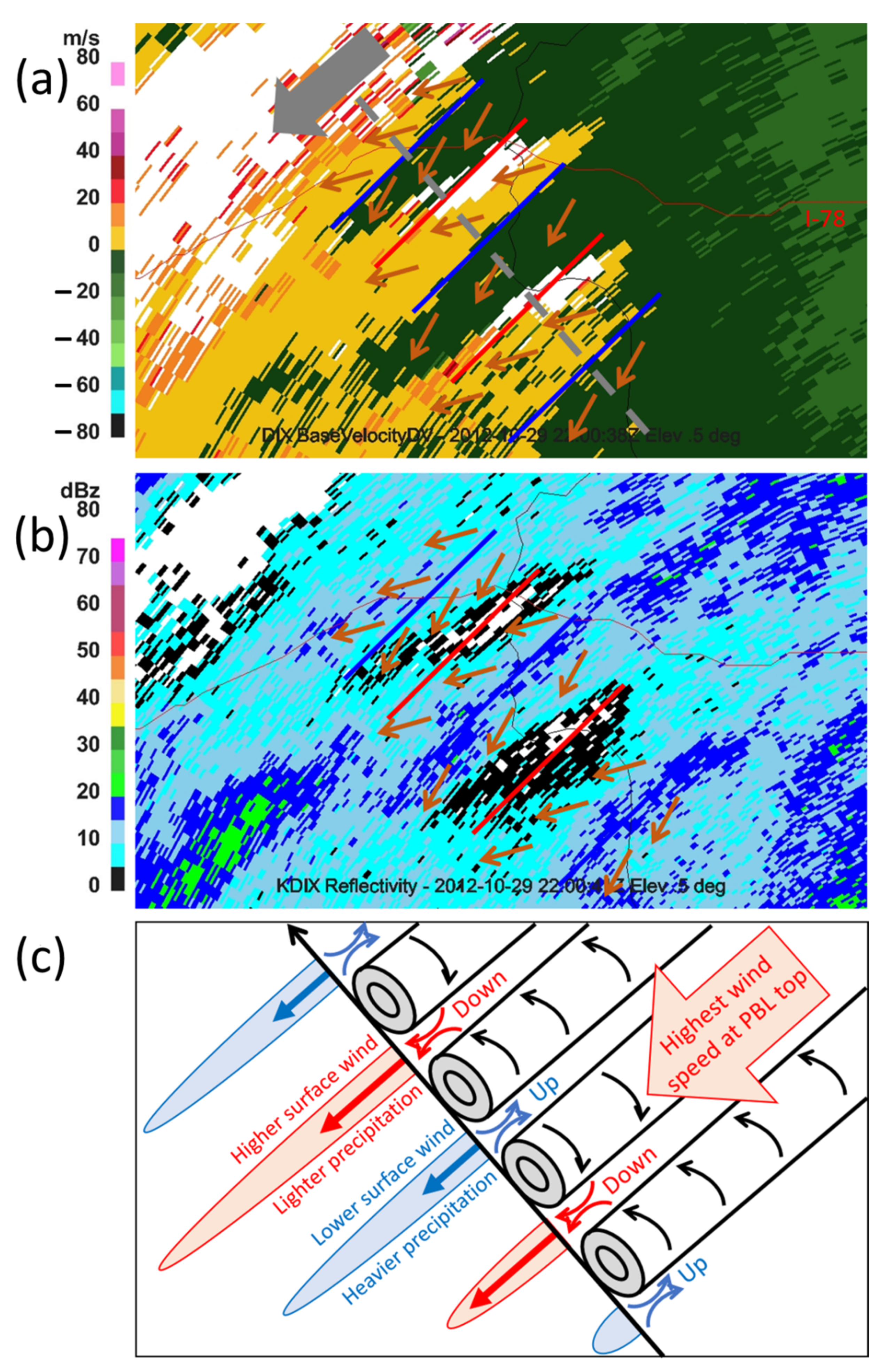
3.1. Radar Observations

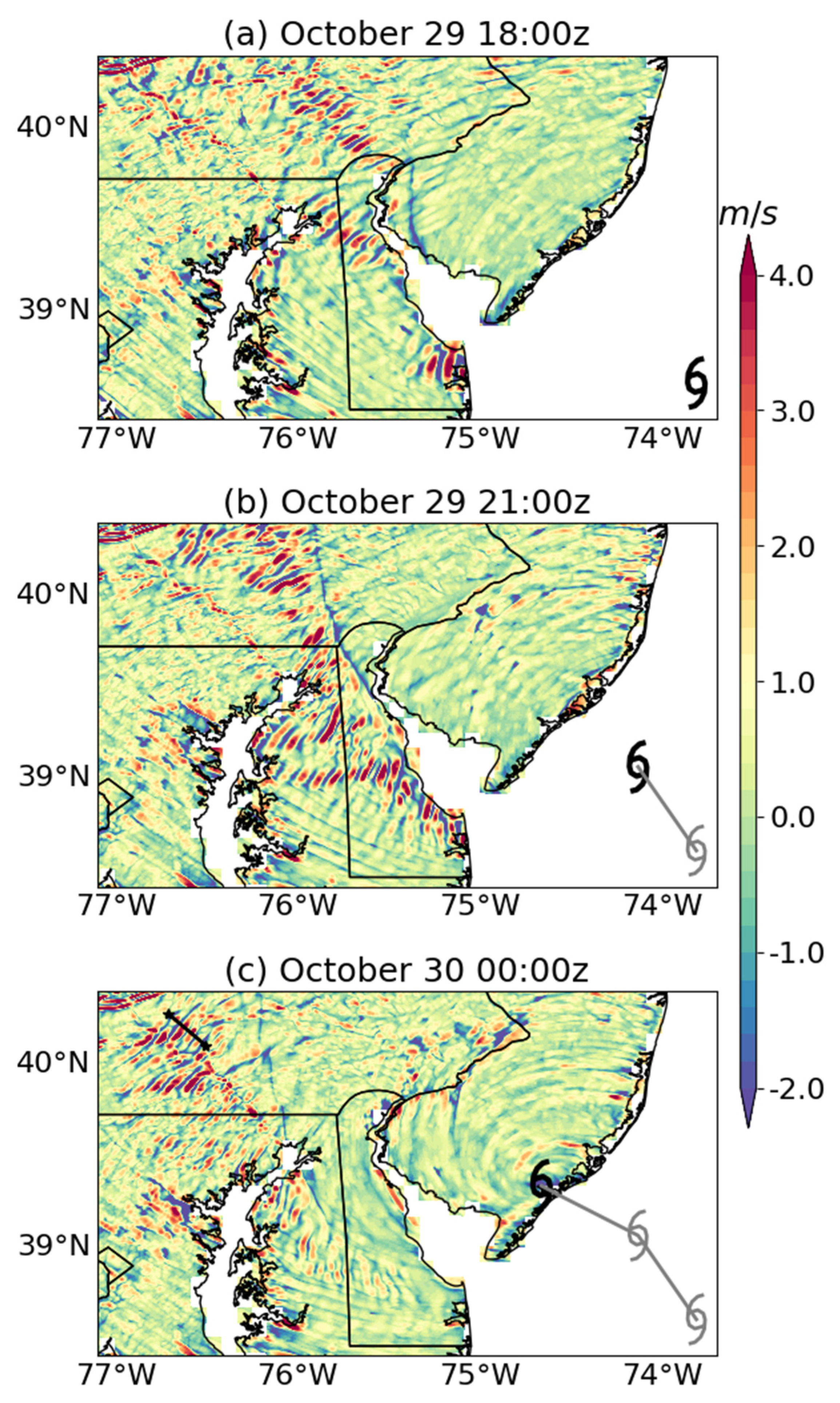
Sandy approached the New Jersey coast as a category 1 hurricane [37] but was reclassified by the National Hurricane Center as a post-tropical cyclone at 2100 UTC 29 October 2012. Landfall occurred near Brigantine, NJ, around 2330 UTC 29 October 2012 with 36 m/s sustained maximum wind and 945 hPa minimum sea-level pressure [22]. Since Sandy’s circulation was rapidly evolving and had become asymmetric by landfall, specifying landfall time under such circumstances is imprecise, so a nominal landfall time of 0000 UTC 30 October 2012 is used herein for convenience when describing features relative to landfall time.

Roll-like signatures were frequently observed by the radar located at Fort Dix, NJ (marked by star in Figure 2), from about 7 h pre-landfall to 6 h post-landfall over a region encompassing parts of New Jersey and eastern Pennsylvania. Figure 2 shows a few consecutive radar images to illustrate the presence of rolls 1 to 2 h prior to landfall. The reflectivity field indicates that deeper and stronger (25–35 dBz) convection occurred in the southwestern portion of each frame, while shallower and weaker (5–20 dBz) precipitation occupied the remainder of the geographical area. The southwestern edge of weaker precipitation represents the westward-advancing warm front, with stronger convection present in advance of the warm front. Roll signatures occurred over a region to the north and east of the deeper and stronger (25–35 dBz) convection. Rolls are distinguishable in radar reflectivity from the chaotic convective cells and turbulence distributed throughout the landfall region by their characteristic elongated linear-shaped features. Longitudinal extent of rolls was typically 50–100 km. The signatures of rolls exhibited in residual velocity images were similar in shape and geographical distribution to those observed in reflectivity images. In regions where rolls existed, alternating lines of enhanced and suppressed reflectivity and residual velocity were apparent. Enhanced and suppressed residual velocities in Figure 2 are consistent with rolls reported in previous studies based on Doppler radar observations [2,3,12,24]. Here, we discovered that rolls can also have an impact on radar reflectivity and thus precipitation intensity.

The vertical circulation of rolls can be inferred from radar radial velocity and reflectivity. To illustrate, a small portion of Figure 2a (black rectangle thereon) is examined in detail in Figure 5. Large-scale wind over this region is approximately in the direction of the thick gray arrow (Figure 5a). If rolls were absent, radar radial velocity would be nearly zero along the plotted radar beam (dashed gray line) because the radar can only detect flow in the direction of the radar beam. However, alternating radar radial velocities were evident along the radar beam, indicating that rolls induced a wind component in the direction of the plotted radar beam. The actual flow (brown arrows) can be qualitatively inferred from the observed radar radial wind. Regions where flow converged (diverged), indicated by blue (red) lines, are areas where strong vertical motion should exist. Indeed, these alternating convergence and divergence zones at 1.5 km height align well with diminished and enhanced precipitation, respectively (Figure 5b). Thus, vertical motion inferred from radar radial velocity is consistent with the alternating features in reflectivity and provides robust evidence of the existence of vertical overturning circulations of rolls. Figure 5c illustrates the roll circulation and its relationship to reflectivity.

The rolls appeared to be grouped into regions, within which roll vortex signatures had similar sizes, orientations, and motions (Figure 2). The longitudinal axes of rolls were oriented roughly parallel to the mean tangential component of the storm’s cyclonic primary circulation (located offshore near the lower right corner of each frame), as found in prior work. As an example, referring to Figure 2e, a roll group comprises the set of alternating red and blue elongated patches oriented along west-southwest to east-northeast axes covering eastern Pennsylvania. The latter axes are the rolls’ longitudinal axes. The roll axes are all linear-shaped rather than arc-shaped, and all linear axes are parallel to each other within each regional group of rolls. Regions that exhibit no linear features, such as northeastern New Jersey, are deemed to be regions without rolls. Propagation of rolls varied, with some propagating colinearly along their longitudinal axis and others propagating at least partially laterally. The manner of propagation, however, was the same within regional groups of rolls (not shown).

Gall et al. [10] and Foster [14] also reported large-scale roll features under tropical cyclones but over water. The large-scale rolls reported here seem distinct from large-aspect ratio roll-like features in Foster [14] because they are linear-shaped rather than arc-shaped as in Foster [14]. In addition, as indicated by the radar images (Figure 2 and Figure 5), the rolls reported here seem to be vertically deeply penetrating rather than capped in the boundary layer. Finally, herein we provide observational insights on the vertical structure of rolls, not just horizonal characteristics.

3.2. WRF Simulation

Rolls identified from radar observations had relatively large spatial scale (further quantified in Section 4.1). Therefore, despite the 500 m WRF resolution and the related caveats described in Section 2.2, the simulation was used to corroborate the presence and qualitative characteristics of the observed roll signatures. The simulation indeed exhibited roll-like signatures similar to observations. Figure 6 displays the simulated perturbation wind speed fields at the lowest model layer over land at 3 h intervals before landfall time. Throughout the geographical domain, wave-like patterns of rolls were evident in the WRF simulation as “footprints” of high and low surface wind speed, which correspond to the descending and ascending arcs of the roll circulation, respectively (Figure 5c). The footprint shapes, orientations, and dimensions were very similar to those of the radar-observed roll signatures, although simulated rolls did not overlap identically with observed rolls in time and place.

4. Roll Size and Formation Mechanism

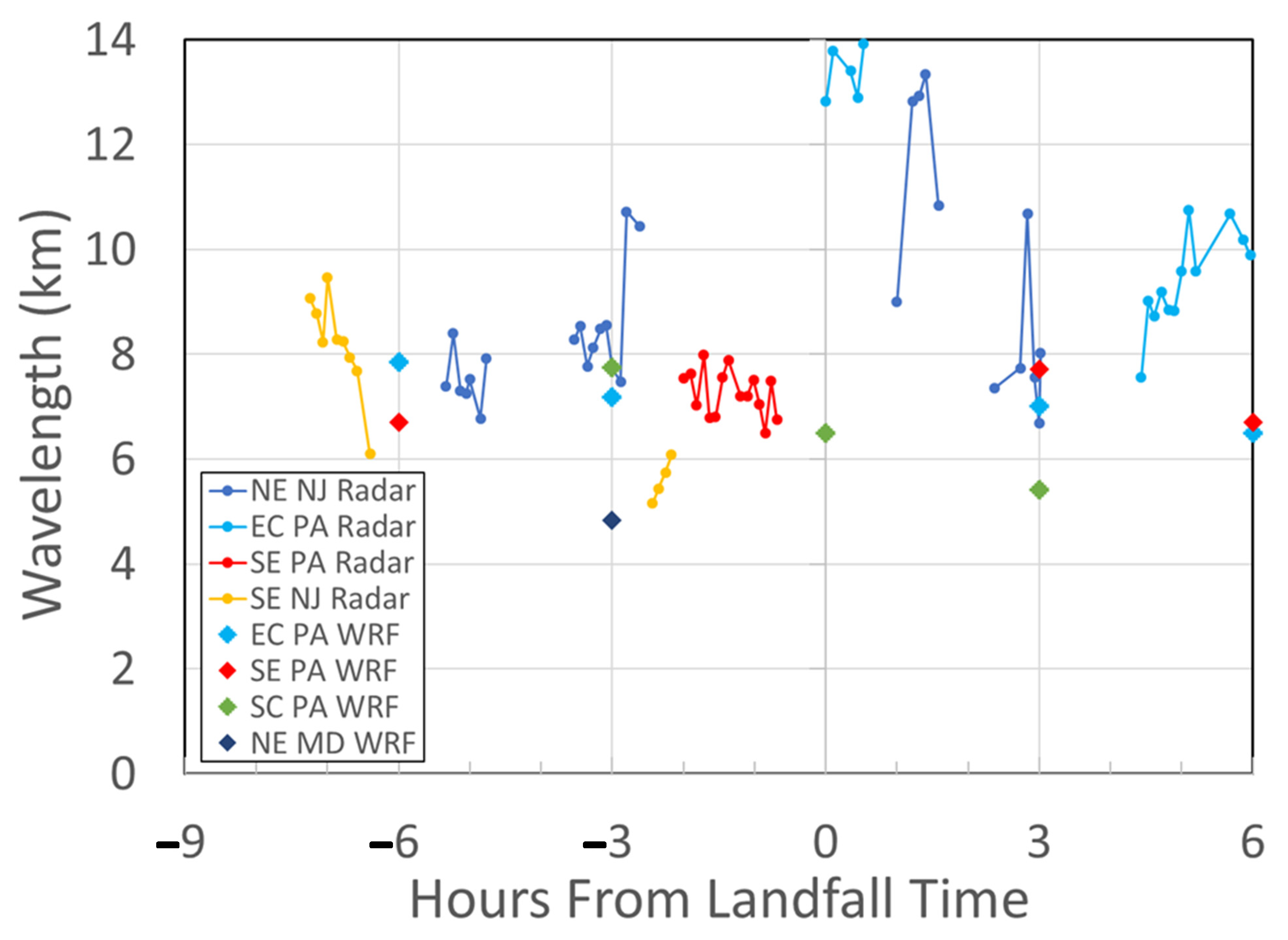
4.1. Horizontal Wavelength

Next, we quantified the spatial scale of rolls using their horizontal wavelength as a metric. We first identified natural regional groupings of rolls that have similar characteristics of size, orientation, and propagation direction. The grouping of rolls, measurement of wavelengths within those groups, and following the groups from one radar scan to another were all done manually, since each group could be clearly identified and followed manually on animations of radar imagery. These groups typically extended over horizontal scales of 50 to 100 km. Wavelength was quantified as average distance between maxima in radar reflectivity for a group of 4 to 8 roll signatures. Typical lifespans of roll groups ranged from 0.5 to 2 h (Figure 7). Roll wavelength from the WRF simulation was obtained in a similar manner, except that it was quantified as distance between maxima in the surface wind speed perturbations. Only rolls presented in three-hourly WRF outputs were analyzed.

Rolls were further classified by their geographical distributions. Radar-observed rolls occurred in four regions (Figure 8a): two were in Pennsylvania, east-central (EC PA) and southeastern (SE PA), and two were in New Jersey, northeastern (NE NJ) and southeastern (SE NJ). The geographical distribution of simulated rolls overlapped partially with the observed ones. Roll signatures were evident in the WRF simulation (Figure 8b) in the two Pennsylvania regions (EC PA and SE PA) where radar exhibited rolls but not evident in the two New Jersey regions (NE NJ and SE NJ). In addition, simulated rolls existed in south-central Pennsylvania (SC PA) and northeastern Maryland (NE MD).

Rolls identified from radar observations had wavelengths ranging from 5 to 14 km, with a mean value of 8.6 km (Figure 7). Previous studies based on radar observations have commonly indicated that rolls have kilometer or subkilometer scales [2,3,12,24]. The linear-shaped rolls observed in this study were therefore significantly larger than those previously reported for a tropical cyclone over land.

Diamonds in Figure 7 show that rolls in the WRF simulation consistently possessed large horizontal scales (which ranged from 5 to 8 km), although they were somewhat smaller than the observed rolls. As noted in Section 2.2 and by Pantillon et al. [19], the simulation’s resolution of 500 m may not suffice to fully resolve rolls of this size, so the wavelengths measured from the WRF simulation must be used with caution. Moreover, because we were not able to pursue any simulation sensitivity analyses of potentially important effects on roll characteristics, such as surface roughness and PBL parameterization, we cannot rule out that the close resemblance of roll signatures manifested by WRF with those observed by radar was coincidental. However, our radar results showed that rolls that were observed over land during TC landfall could be substantially larger than those reported previously.

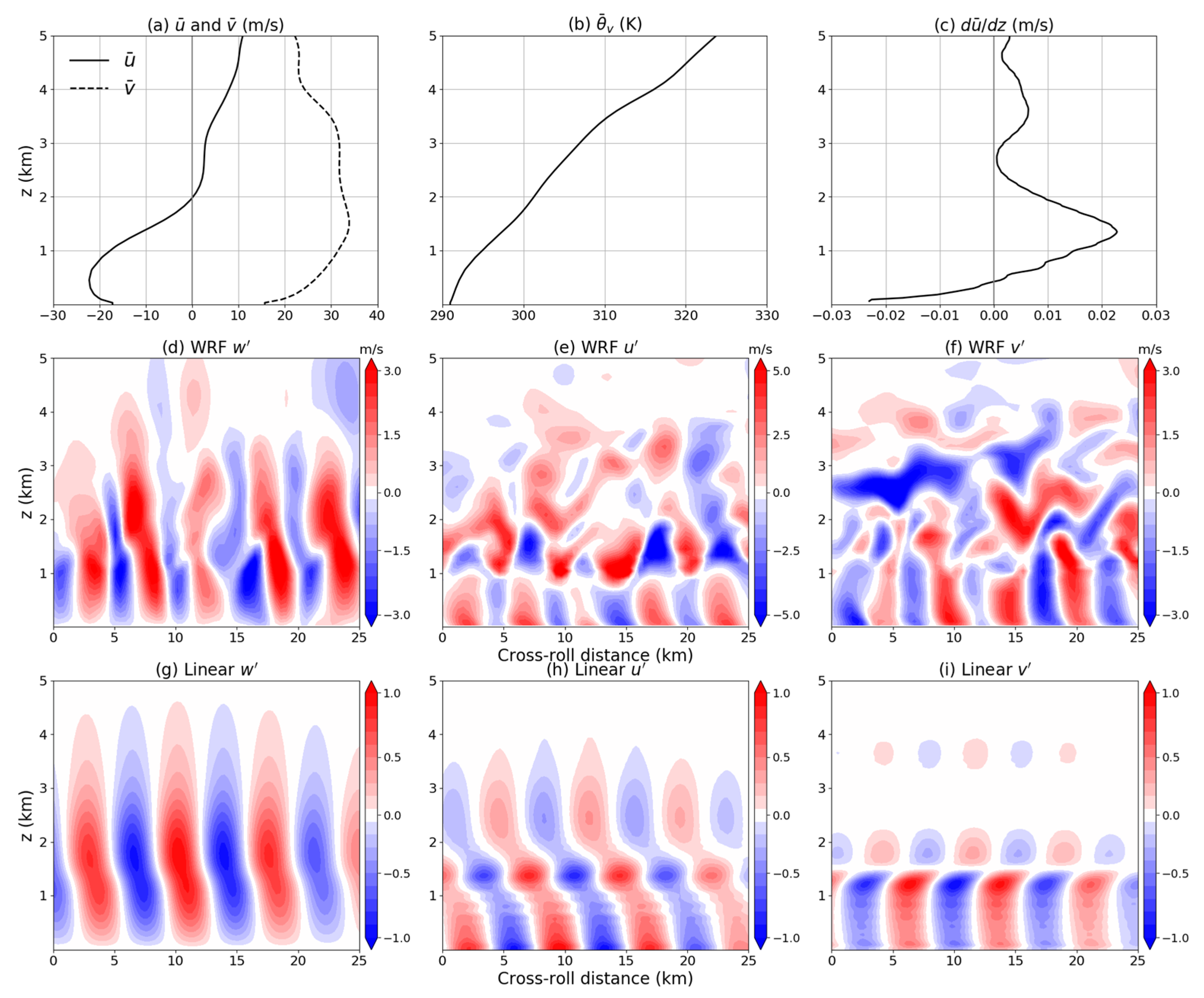
4.2. Roll Structure and Formation Mechanism

The WRF simulation reproduced the gross features of rolls exhibited in observations and thus offered an opportunity to explore the roll formation mechanism. Figure 9 illustrates an example of the simulated roll structure along a cross section in the TC radial direction, together with mean flow profiles obtained as a 50 × 50 km area mean. Rolls were characterized by deep-penetrating overturning circulations reaching up to 4 km height (Figure 5d–e). Alternating tangential wind perturbations were associated with overturning circulations (Figure 9f). All of these features were consistent with the typical structure of rolls inferred from previously reported radar observations (e.g., Morrison et al. [24]), idealized models (e.g., Gao and Ginis [36]), and large eddy simulation studies (e.g., Wang and Jiang [38]), except that the spatial scale of rolls reported herein was much larger.

The rolls under hurricane conditions are commonly thought to be driven by the dynamical instability associated with the radial wind distribution. Therefore, we further examined whether this was the case for the larger-scale rolls identified here. The mean environment in the roll formation region was typically characterized by negative surface heat flux and a stable near-surface stratification (Figure 9b), suggesting that the rolls were not forced by surface buoyancy fluxes. The mean radial wind was characterized by an inflection point, where radial wind shear reached a maximum value (Figure 9c), implying that rolls were formed by the inflection-point instability associated with radial wind [21,36]. The radial wind shear had a noticeably deep layer with positive shear (~2 km vertically; Figure 9c). Gao and Ginis [39] found that the roll spatial scale is proportional to shear layer depth (SLD), defined as the depth of the layer over which vertical shear of the radial wind component is positive. The large rolls described here were therefore possibly due to the deep shear layer.

To validate this hypothesis, we obtained the linear-phase rolls with the linearized roll model (Section 2.3) driven by the mean flow profiles (Figure 9a–c). The linear roll solution was not expected to resemble exactly those in observations or in a full-physics simulation since nonlinear terms were not considered. Nevertheless, the solution from the linearized roll model (Figure 9g–i) exhibited many features similar to those of the WRF simulation (Figure 9d–f). In addition, the spatial scale of rolls was consistent with, although somewhat larger than, that from WRF. This supports the hypothesis that large-scale rolls manifested by the WRF simulation were formed due to the inflection point instability associated with the deep radial shear layer.

4.3. Mean Environment

The horizontal distribution of SLD showed that the deep radial shear layer (~2 km thick) existed over land in the WRF simulation (Figure 10). The deep shear under Sandy during the landfall period was likely responsible for the large rolls observed. The formation of the deep shear layer could be due to the warm front or wind structure changes during landfall. To show that the simulated deep wind shear layer is not an artifact, we next examined the radar VAD wind profiles at Fort Dix, NJ, to explore the temporal variation in the observed radial and tangential wind profiles north of the storm center as it traversed southern New Jersey.

Sixteen hourly VAD wind profiles were examined beginning at 1500 UTC 29 October 2012, which spanned 9 h before to 6 h after landfall. Radar wind profile observations require precipitation echoes, and they reached at least a height of 7 km throughout the 15 h time span of the hourly profiles, except for the 2200–0100 UTC interval, wherein their tops dropped to as low as 2.4 km at 2300 and 0000 UTC. Figure 11a shows two sets of wind profiles selected as the earliest examined (1501 UTC) and the maximum depth of the layer of positive radial wind shear (1903 UTC, per discussion below on Figure 11b). Three plots are shown on each frame: storm-motion-corrected radial and tangential wind components and vertical shear of the radial wind component. The profiles clearly show the strong, deep inflow below 2 km elevation (blue), the strong maximum tangential wind component near 1.5 km elevation (red), and the deep layer of positive radial wind shear (gray).

Figure 11a illustrates that both the layer depth and maximum magnitude of the inward radial velocity increased over the 4 h between the two sets of profiles. Therefore, time series of these variables are plotted in Figure 11b,c, where the time scale is in hours relative to landfall time, analogous to that for Figure 7. The blue plot in Figure 11b shows the radial wind SLD as defined in Figure 4b of Gao and Ginis [38], i.e., the vertical extent of positive radial wind shear. Note that for times after 0100 UTC, there was no inward wind component despite positive shear at these times. The red plot shows the distance of the storm center from the radar VAD observation site as Sandy traversed west-northwestward across southern New Jersey. The airstream bands at the bottom of the plot denote the periods during which the radar site was within the southward-advancing cold conveyor belt (CCB) airstream (left blue band), the southwestward-advancing warm conveyor belt (WCB) airstream (pink band), and the northwestward-advancing CCB secluding airstream (right blue band). Figure 11c shows the maximum inward radial velocity. As in Figure 11b, after 0100 UTC, there was no inward wind component, which is why no points are plotted there.

Interestingly, various features of the pair of time series plots corresponded to Sandy’s airstreams. The maximum SLD at 5 h before landfall (Figure 11b) and the maximum tangential velocity (not shown) both occurred while the radar site was under the stronger convection of the southwestward-advancing warm frontal zone. Prior to that time, the radar site was in the northerly CCB airstream. Furthermore, the profile’s radial shear at this time exhibited a secondary maximum at 4 km elevation, which was above the primary maximum at 1.4 km and which contributed to the large vertical extent of positive radial shear. Perhaps this double feature and deep SLD is due to the WCB airstream overrunning the CCB airstream or possibly simply due to the deeper convection at the warm frontal zone. Finally, the highest inflow layer velocities (Figure 11c) and tops (not shown) occurred while the radar site was within the southwestward-flowing WCB. The inflow layer maximum speed dropped dramatically approaching landfall time as the warm core became fully secluded by the cold airstream; by an hour after landfall, low-level inflow was absent. Finally, there was an elevated positive radial wind shear layer between 1.9 and 3.2 km elevation during 2 to 6 h after landfall time.

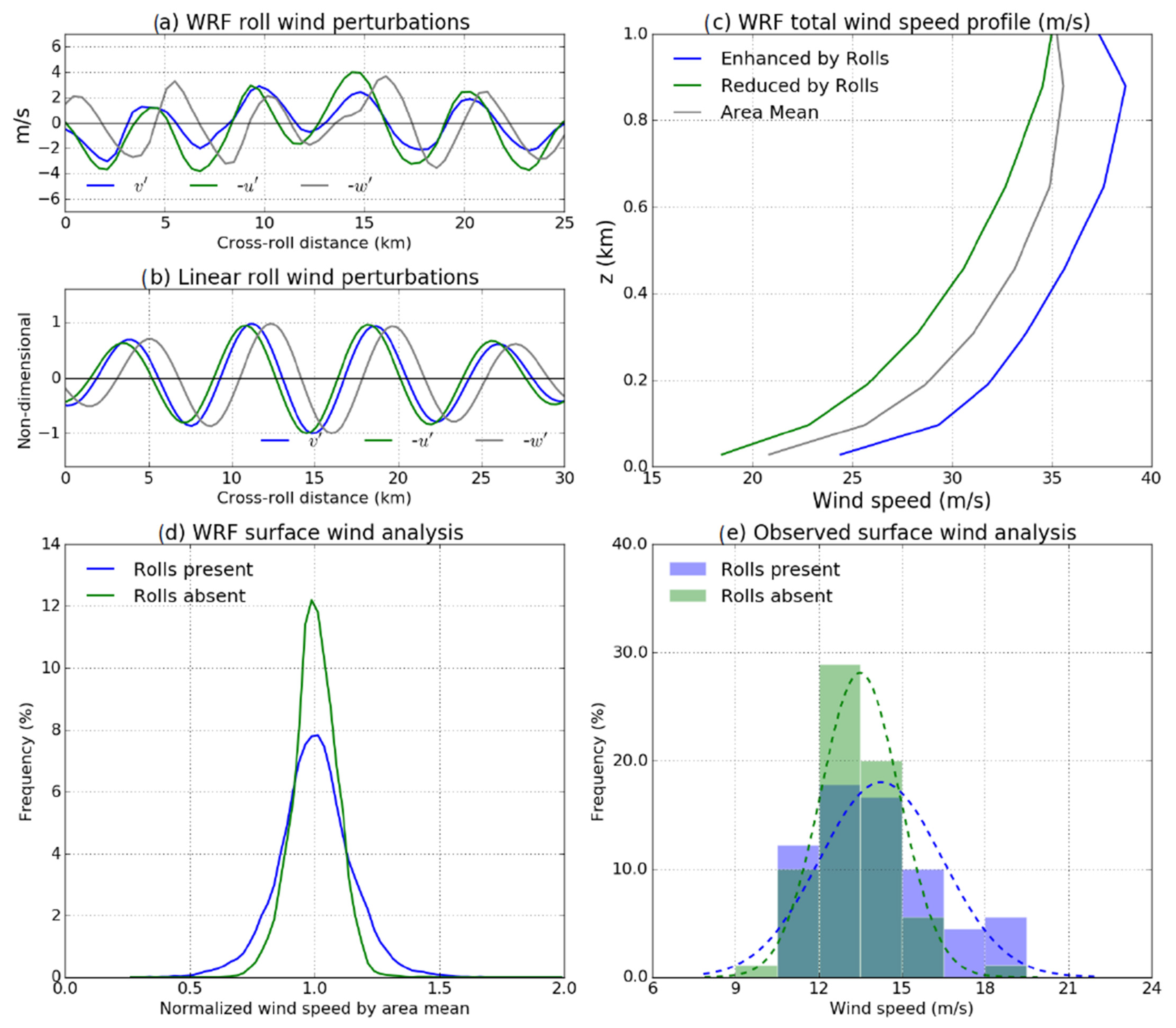
5. Impact of Rolls on Surface Wind Speed

Here, we quantified the impact of rolls on the probability of hazardous surface winds based on the WRF simulation and best available observations collected during Sandy’s landfall. We began with examining the distribution of surface wind perturbations across the rolls as seen in the WRF simulation. Interestingly, as shown in Figure 12a, areas where surface tangential winds were enhanced (positive v′) approximately overlapped with the areas with enhanced surface radial wind (negative u′). This indicated that the roll-induced tangential and radial wind perturbations acted in concert to contribute to total surface wind speed enhancement. The peak of enhanced total wind speed was shifted to the storm-center side of peak downdrafts. Such a distribution is consistent with results from the linearized roll model (Figure 12b). Due to the deep extent of rolls, their impact on total wind speed was persistent over height in the PBL (below 1 km height; Figure 12c).

It is expected that there is significantly increased likelihood for some regions to experience more hazardous winds when rolls are present. We next quantified the roll contribution to the likelihood of surface wind speed noticeably exceeding the regional mean speed based on the WRF surface wind field. For this purpose, we analyzed and compared the surface wind field over regions with rolls and over neighboring regions with similar mean wind speed but lacking roll signatures (Figure 8b). Prior to calculating probability density functions (PDFs), the wind speed for each region was normalized by the regional mean value so that regional wind speed data could be aggregated into a single set. Figure 12d shows PDFs of normalized surface wind speed in regions with and without rolls. Roll regions had noticeably wider distributions and higher maximum wind speeds than non-roll regions. Quantitatively, WRF output indicated that it was about 30 times more likely for the wind speed to exceed 40% above mean speed in roll regions compared to non-roll regions. Thus, the WRF surface wind fields illustrated that when rolls were present, they contributed to a broader wind speed probability distribution and significantly increased the likelihood of higher, more hazardous wind speeds.

When rolls laterally propagate, they modulate the wind speed observed at a fixed location. However, observing wind speed periodicity caused by rolls is very challenging as it requires high-frequency measurements at the location experiencing laterally propagating rolls. During Sandy’s landfall period, only the NOAA Automated Surface Observing System [40] station located at Teterboro, NJ, satisfied this requirement, i.e., propagating rolls occurring at Teterboro when 1 min observations were available there. Furthermore, only a single pair of 1 h windows, within which one clearly exhibited roll signatures and the other clearly did not, was available for analysis. Thus, the histograms of 10 m wind speed (2 min mean) measured at Teterboro during these two nonconsecutive one-hour windows shown in Figure 12e, one with propagating rolls and one without, are intended only as an illustrative example of the possible impact of propagating rolls on wind speed observations at a fixed location. These two periods have similar mean wind speed (14.2 and 13.5 m/s, respectively) but are separated by 3 h in time, so causes of the differences in wind speed distributions beyond roll propagation, such as structural changes in the storm, cannot be ruled out.

6. Summary

One important aspect of hurricane research is forecasting and understanding wind damage during hurricane landfall. Boundary layer rolls act as an important mechanism in transporting high momentum air downward and causing localized elongated damage swaths. Characterizing rolls and mechanisms that drive them is also important for improving hurricane intensity forecasts because hurricane intensification is impacted by roll vortices’ transport of momentum and enthalpy vertically through the hurricane boundary layer. Given that the current understanding of rolls is restrained by the limited availability of direct observations, this work builds upon prior observational case studies by contributing new observational evidence for an uncommon case of large-scale rolls that occurred over land during the late stage of TC extratropical transition. Specifically, we highlighted the occurrence of large-scale rolls over land during landfall of Post-Tropical Cyclone Sandy. Many roll characteristics from radar reflectivity, radar velocity, and surface wind speed observations were corroborated by the 500 m resolution WRF simulation. The spatial scale of rolls (5–14 km horizontal wavelength) determined from radar observations was larger than any previously published for a tropical cyclone over land. Radar reflectivity showed analogous alternating lines of diminished and enhanced precipitation implicitly found to be associated with the downward and upward portions of the roll circulations, respectively.

The 500 m resolution WRF simulation exhibited similar roll features over land. High-speed surface wind footprints were exhibited in the WRF simulation, which were associated with roll downdrafts. Analyses of surface wind speed in WRF and limited in situ observations consistently showed that rolls significantly increased the likelihood of hazardous winds near the ground and likely contributed to patchy treefall observed throughout Sandy’s landfall region.

Quantifying and characterizing rolls for this case study was limited to the types of analyses reported herein by the availability of observations and the use of archived WRF simulation output. Surface wind observations were limited by both storm-caused data outages and observation temporal resolution, while vertical profile observations were limited by absence of such observational sites in the landfall region. Although the archived WRF simulation did use a high resolution 500 m grid spacing and reproduced many of the features of the observed rolls, the spacing was admittedly marginal for reproducing rolls having wavelengths comparable to the observed wavelengths of 5–14 km. Moreover, the use of archived simulation output prevented conducting simulation sensitivity studies.

The large size of tropical cyclone rolls reported here is consistent with the shear layer depth parameter of Gao and Ginis [39] that drives roll spatial scale. The large shear layer depth of radial wind in the WRF simulation may be attributable to Sandy’s high latitude, the strong warm front, or wind structure changes during landfall. The roles of these possible mechanisms and characteristics in contributing to the large size of rolls in Sandy will be studied in subsequent analyses using large eddy simulations.

References

1. Greenberg, C.H.; McNab, W. Forest disturbance in hurricane-related downbursts in the Appalachian mountains of North Carolina. For. Ecol. Manag. 1998, 104, 179–191. [Google Scholar] [CrossRef]
2. Wurman, J.; Winslow, J. Intense Sub-Kilometer-Scale Boundary Layer Rolls Observed in Hurricane Fran. Science 1998, 280, 555–557. [Google Scholar] [CrossRef] [PubMed]
3. Ellis, R.; Businger, S. Helical circulations in the typhoon boundary layer. J. Geophys. Res. Space Phys. 2010, 115, 06205. [Google Scholar] [CrossRef] [Green Version]
4. Kuettner, J. The Band Structure of the Atmosphere. Tellus 1959, 11, 267–294. [Google Scholar] [CrossRef]
5. Walter, B.A.; Overland, J.E. Observations of Longitudinal Rolls in a Near Neutral Atmosphere. Mon. Weather Rev. 1984, 112, 200–208. [Google Scholar] [CrossRef] [Green Version]
6. Kelly, R.D. Horizontal Roll and Boundary-Layer Interrelationships Observed over Lake Michigan. J. Atmos. Sci. 1984, 41, 1816–1826. [Google Scholar] [CrossRef]
7. Christian, T.W.; Wakimoto, R.M. The Relationship between Radar Reflectivities and Clouds Associated with Horizontal Roll Convection on 8 August 1982. Mon. Weather Rev. 1989, 117, 1530–1544. [Google Scholar] [CrossRef] [Green Version]
8. Etling, D.; Brown, R.A. Roll vortices in the planetary boundary layer: A review. Bound.-Layer Meteorol. 1993, 65, 215–248. [Google Scholar] [CrossRef]
9. Young, G.S.; Kristovich, D.A.R.; Hjelmfelt, M.R.; Foster, R.C. Rolls, Streets, Waves, and More: A Review of Quasi-Two-Dimensional Structures in the Atmospheric Boundary Layer. Bull. Am. Meteorol. Soc. 2002, 83, 997–1001. [Google Scholar] [CrossRef]
10. Gall, R.; Tuttle, J.; Hildebrand, P. Small-scale spiral bands observed in Hurricanes Andrew, Hugo, and Erin. Mon. Wea. Rev. 1998, 126, 1749–1766. [Google Scholar] [CrossRef]
11. Nolan, D.S. Instabilities in hurricane-like boundary layers. Dyn. Atmos. Oceans 2005, 40, 209–236. [Google Scholar] [CrossRef]
12. Lorsolo, S.; Schroeder, J.L.; Dodge, P.; Marks, F. An Observational Study of Hurricane Boundary Layer Small-Scale Coherent Structures. Mon. Weather Rev. 2008, 136, 2871–2893. [Google Scholar] [CrossRef]
13. Zhang, J.A.; Katsaros, K.B.; Black, P.G.; Lehner, S.; French, J.R.; Drennan, W.M. Effects of Roll Vortices on Turbulent Fluxes in the Hurricane Boundary Layer. Boundary-Layer Meteorol. 2008, 128, 173–189. [Google Scholar] [CrossRef]
14. Foster, R. Signature of Large Aspect Ratio Roll Vortices in Synthetic Aperture Radar Images of Tropical Cyclones. Oceanography 2013, 26, 58–67. [Google Scholar] [CrossRef]
15. Ito, J.; Oizumi, T.; Niino, H. Near-surface coherent structures explored by large eddy simulation of entire tropical cyclones. Sci. Rep. 2017, 7, 3798. [Google Scholar] [CrossRef] [Green Version]
16. Zhu, P. Simulation and parameterization of the turbulent transport in the hurricane boundary layer by large eddies. J. Geophys. Res. Space Phys. 2008, 113, D17. [Google Scholar] [CrossRef]
17. Nakanishi, M.; Niino, H. Large-Eddy Simulation of Roll Vortices in a Hurricane Boundary Layer. J. Atmos. Sci. 2012, 69, 3558–3575. [Google Scholar] [CrossRef]
18. Green, B.W.; Zhang, F. Idealized Large-Eddy Simulations of a Tropical Cyclone–like Boundary Layer. J. Atmos. Sci. 2015, 72, 1743–1764. [Google Scholar] [CrossRef] [Green Version]
19. Pantillon, F.; Adler, B.; Corsmeier, U.; Knippertz, P.; Wieser, A.; Hansen, A. Formation of Wind Gusts in an Extratropical Cyclone in Light of Doppler Lidar Observations and Large-Eddy Simulations. Mon. Weather Rev. 2019, 148, 353–375. [Google Scholar] [CrossRef]
20. Mourad, P.D.; Brown, R.A. Multiscale Large Eddy States in Weakly Stratified Planetary Boundary Layers. J. Atmos. Sci. 1990, 47, 414–438. [Google Scholar] [CrossRef] [Green Version]
21. Foster, R.C. Why Rolls are Prevalent in the Hurricane Boundary Layer. J. Atmos. Sci. 2005, 62, 2647–2661. [Google Scholar] [CrossRef]
22. Blake, E.S.; Kimberlain, T.B.; Berg, R.J.; Cangialosi, J.P.; Beven, J.L., III. Tropical Cyclone Report: Hurricane Sandy; Tech. Rep. AL182012; NOAA/National Hurricane Center: Miami, FL, USA, 2013; 157p.
23. NOAA National Weather Service (NWS) Radar Operations Center. NOAA Next Generation Radar (NEXRAD) Level 2 Base Data. Products N0U, N0Q. 1991. Available online: https://www.ncei.noaa.gov/access/metadata/landing-page/bin/iso?id=gov.noaa.ncdc:C00345 (accessed on 18 June 2019).
24. Morrison, I.; Businger, S.; Marks, F.; Dodge, P.; Businger, J.A. An Observational Case for the Prevalence of Roll Vortices in the Hurricane Boundary Layer. J. Atmos. Sci. 2005, 62, 2662–2673. [Google Scholar] [CrossRef] [Green Version]
25. Chrisman, J.N.; Smith, S.D. Enhanced velocity azimuth display wind profile (EVWP) function. In Proceedings of the 34th Conference on Radar Meteorology, Williamsburg, VA, USA, 5–9 October 2009. [Google Scholar]
26. Wyngaard, J.C. Toward numerical modeling in the “terra incognita”. J. Atmos. Sci. 2004, 61, 1816–1826. [Google Scholar] [CrossRef]
27. Haupt, S.E.; Kosovic, B.; Shaw, W.; Berg, L.K.; Churchfield, M.; Cline, J.; Draxl, C.; Ennis, B.; Koo, E.; Kotamarthi, R.; et al. On Bridging A Modeling Scale Gap: Mesoscale to Microscale Coupling for Wind Energy. Bull. Am. Meteorol. Soc. 2019, 100, 2533–2550. [Google Scholar] [CrossRef]
28. LeMone, M.A.; Angevine, W.M.; Bretherton, C.S.; Chen, F.; Dudhia, J.; Fedorovich, E.; Katsaros, K.B.; Lenschow, D.H.; Mahrt, L.; Patton, E.G.; et al. 100 Years of Progress in Boundary Layer Meteorology. Meteorol. Monogr. 2019, 59, 9.1–9.85. [Google Scholar] [CrossRef]
29. Johnsen, P.; Straka, M.; Shapiro, M.; Norton, A.; Galarneau, T. Petascale WRF simulation of Hurricane Sandy: Deployment of NCSA’s Cray XE6 Blue Waters. In Proceedings of the SC13: International Conference for High Performance Computing, Networking, Storage and Analysis, Denver, CO, USA, 17–21 November 2013; IEEE: New York, NY, USA, 2014. [Google Scholar]
30. Hong, S.-Y.; Noh, Y.; Dudhia, J. A New Vertical Diffusion Package with an Explicit Treatment of Entrainment Processes. Mon. Weather Rev. 2006, 134, 2318–2341. [Google Scholar] [CrossRef] [Green Version]
31. Skamarock, W.C.; Klemp, J.B.; Dudhia, J.; Gill, D.O.; Barker, D.M.; Wang, W.; Powers, J.G. A Description of the Advanced Research WRF Version 3; NCAR Technical Note NCAR/TN-475+STR; National Center for Atmospheric Research: Boulder, CO, USA, 2008. [Google Scholar]
32. Zhang, D.; Anthes, R.A. A High-Resolution Model of the Planetary Boundary Layer—Sensitivity Tests and Comparisons with SESAME-79 Data. J. Appl. Meteorol. 1982, 21, 1594–1609. [Google Scholar] [CrossRef]
33. Wu, L.; Liu, Q.; Li, Y. Tornado-scale vortices in the tropical cyclone boundary layer: Numerical simulation with the WRF–LES framework. Atmos. Chem. Phys. Discuss. 2019, 19, 2477–2487. [Google Scholar] [CrossRef] [Green Version]
34. Hong, S.Y.; Lim, J.O.J. The WRF single-moment 6-class microphysics scheme (WSM6). J. Korean Meteor. Soc. 2006, 42, 129–151. [Google Scholar]
35. Schiavone, J.A.; Johnsen, P.J. High resolution WRF simulation of Hurricane Sandy (2012) wind during landfall. Zenodo 2020. [Google Scholar] [CrossRef]
36. Gao, K.; Ginis, I. On the Generation of Roll Vortices due to the Inflection Point Instability of the Hurricane Boundary Layer Flow. J. Atmos. Sci. 2014, 71, 4292–4307. [Google Scholar] [CrossRef] [Green Version]
37. Simpson, R.H. The hurricane disaster potential scale. Weatherwise 1974, 27, 169–186. [Google Scholar]
38. Wang, S.; Jiang, Q. Impact of vertical wind shear on roll structure in idealized hurricane boundary layers. Atmos. Chem. Phys. Discuss. 2017, 17, 3507–3524. [Google Scholar] [CrossRef] [Green Version]
39. Gao, K.; Ginis, I. On the Characteristics of Linear-Phase Roll Vortices under a Moving Hurricane Boundary Layer. J. Atmos. Sci. 2018, 75, 2589–2598. [Google Scholar] [CrossRef]
40. NOAA National Climatic Data Center. 1-Minute ASOS Data. 2019. Available online: ftp://ftp.ncdc.noaa.gov/pub/data/asos-onemin/ (accessed on 12 May 2018).
Figure 1. Landsat images comparing the treefall pattern after Sandy’s landfall with those before landfall at two locations: Bridgewater and Somerset, NJ. Arrow length and direction indicate treefall patch extent and treefall direction, respectively. Map data ©2013 Google.
Atmosphere 12 00259 g001
Figure 2. Roll signatures in observations during Sandy’s landfall period obtained by WSR-88D radar located at Fort Dix, NJ. All radar scans are at an elevation angle of 0.5 degree, which is the lowest angle available. Radar location is indicated by the black star. Distance from Sandy’s center is shown as contour lines (100 to 250 km with an interval of 50 km). Figure (a,c,e,g) shows radar residual velocity at 2200, 2217, 2233, and 2254 UTC 29 October 2012, respectively. Figure (b,d,f,h) shows reflectivity at 2200, 2217, 2233, and 2254 UTC, respectively. The color bar for reflectivity is chosen to emphasize roll features. The height above ground of the measured wind component increases with distance from the radar site, from about 0.7 km height near the roll features in southwestern New Jersey to about 3.9 km at the northwestern edge of the roll features over eastern Pennsylvania.
Atmosphere 12 00259 g002
Figure 3. A demonstration of Fourier analysis of the radar radial velocity. (a) The total radar radial velocity. (b) Comparison between the total radar radial velocity and the first harmonic obtained using the Fourier analysis at a radius of 25 km. (c) The radar residual velocity obtained by subtracting the first harmonic from the total radar residual velocity.
Atmosphere 12 00259 g003
Figure 4. Comparison of actual and simulated storm center tracks. Red lines denote actual track based on National Hurricane Centre (NHC) best track data [22], and blue lines denote Weather Research and Forecasting (WRF)-simulated track indicated by the position of the minimum sea level pressure.
Atmosphere 12 00259 g004
Figure 5. The radar (a) radial velocity and (b) reflectivity for the region identified by the black rectangle on Figure 2a,b. The radar site is located about 80 km southeast of the region shown. Elevation of the radar scan within this region is about 1.5 km height. The approximate mean wind direction is indicated by the thick gray arrow. Yellow (green) in (a) indicates a flow component away from (toward) the radar site. Brown arrows in (a,b) indicate, qualitatively, the horizontal flow direction inferred from the radar radial velocity. Blue (red) lines in (a,b) indicate areas of convergence (divergence). Figure (c) shows a conceptual diagram of rolls. Elliptical cylinders represent rolls, and the curved red (blue) arrows between rolls represent downward (upward) motions. The red and blue shaded patches indicate impacts of rolls on total surface wind speed and precipitation.
Atmosphere 12 00259 g005
Figure 6. The WRF wind speed perturbations at about 30 m height before Sandy’s landfall time. Red (blue) indicates enhanced (diminished) wind speed. Tropical cyclone symbols indicate the storm center, with the bold symbol denoting storm center location at the time of each frame. Only wind speed perturbations over land are shown to highlight the presence of roll perturbations over land. Figure (ac) shows WRF wind speed perturbations at 1800 UTC 29 October 2012, 2100 UTC 29 October 2012, and 0000 UTC 30 October 2012, respectively.
Atmosphere 12 00259 g006
Figure 7. The roll wavelengths quantified based on radar observations (points and solid lines) and from Weather Research and Forecasting (WRF) simulation (diamonds) for regions where rolls were prevalent and plotted versus time relative to landfall time.
Atmosphere 12 00259 g007
Figure 8. Regions used for roll wavelength measurements shown in Figure 7 and for WRF surface wind speed probability density function (PDF) analysis discussed in Section 5. (a) Regions used for radar-observed wavelength analysis. (b) Regions used for WRF roll wavelength and wind speed PDF analysis, where solid (dashed) lines denote 50 × 50 km regions exhibiting the presence (absence) of rolls. Line colors identify the WRF time steps.
Atmosphere 12 00259 g008
Figure 9. Simulated roll structure at 0000 UTC 30 October 2012 for transect line shown in Figure 6c. The radial (u) and tangential (v) wind components are projected onto storm-centered cylindrical coordinates. Figure (ac) shows area-averaged vertical profiles of horizontal velocity components, virtual potential temperature, and radial wind shear, respectively, from the WRF simulation. Figure (df) shows cross sections of vertical, radial, and tangential velocity perturbations associated with rolls, respectively. Figure (gi) shows cross sections analogous to those shown for WRF except that they are from the linearized roll model. The cross sections extend outward from the storm center so the 0 and 25 km end points represent the east-northeast (ESE) and west-northwest (WNW) transect end points, respectively.
Atmosphere 12 00259 g009
Figure 10. The radial wind shear layer depth (SLD) as simulated in WRF at 0000 UTC 30 October 2012.
Atmosphere 12 00259 g010
Figure 11. Vertical wind profiles observed at Fort Dix, NJ, by the Doppler radar using its velocity azimuth display (VAD) algorithm. (a) Vertical profiles of radial (blue) and tangential (red) wind components relative to the moving storm center and of the vertical shear of the radial wind component (gray). Units of the latter are 0.001/s. (b) Time series of hourly observations of radial wind shear layer depth (blue), top of radar echoes (yellow), and distance of storm center from radar site (red) with units in km/100. Horizontal colored bands above time scale denote when the radar site was within CCB (blue) and WCB (pink) airstreams. (c) Similar to (b) except that blue represents maximum inward radial velocity and storm distance units are km/10.
Atmosphere 12 00259 g011
Figure 12. Impact of rolls on total surface wind speed. (a) The roll-induced tangential (v′) and radial (u′) wind speed perturbations at the lowest model level (approximately 30 m height) and the roll vertical velocity at 1 km height (w′) corresponding to the WRF cross sections shown in Figure 9d–f. Note the signs of u′ and w′ are reversed to better reveal the phase difference relative to v′. (b) Similar to (a) but from the linearized roll model as shown in Figure 9g–i. The three wind components from the linear model are normalized by their maximum values, respectively. (c) Representative profiles of total wind speed at the grid points where surface wind speed is enhanced and reduced by rolls in WRF, respectively. The gray line shows area mean profile for comparison. The data used for the analysis in (ac) are the same as in Figure 9. (d) Probability density functions of surface wind speed in areas with and without rolls estimated from the WRF simulation (areas shown in Figure 8b). (e) Histograms of 10 m height wind observations measured at the National Oceanic and Atmospheric Administration (NOAA) Automated Surface Observing System station at Teterboro, NJ, during the periods with (blue color) and without (green color) propagating rolls. The overlapped areas are indicated by the dark color.
Atmosphere 12 00259 g012
Publisher’s Note: MDPI stays neutral with regard to jurisdictional claims in published maps and institutional affiliations.