Article

El Niño-Southern Oscillation and Indian Ocean Dipole Modes: Their Effects on South American Rainfall during Austral Spring

by
Mary T. Kayano
1,*,
Wilmar L. Cerón
2,
Rita V. Andreoli
3,4,
Rodrigo A. F. Souza
3,
Itamara P. Souza
3,4 and
Teresita Canchala
5
1
Coordenação Geral de Ciências da Terra, Instituto Nacional de Pesquisas Espaciais, Avenida dos Astronautas, 1758, São José dos Campos 12227-010, SP, Brazil
2
Department of Geography, Faculty of Humanities, Universidad del Valle, Calle 13 # 100-00, Cali P.O. Box 25360, Colombia
3
Escola Superior de Tecnologia, Universidade do Estado do Amazonas, Avenue Darcy Vargas, 1200, Parque 10 de Novembro, Manaus 69065-020, AM, Brazil
4
Programa de Pós-Graduação em Clima e Ambiente, Instituto Nacional de Pesquisa da Amazonia/Universidade do Estado do Amazonas, Avenue André Araújo, 2936, Manaus 69060-001, AM, Brazil
5
Water Resources Engineering and Soil Research Group, School of Natural Resources and Environmental Engineering, Universidad del Valle, Calle 13 # 100-00, Cali P.O. Box 25360, Colombia
*
Author to whom correspondence should be addressed.
Atmosphere 2021, 12(11), 1437; https://doi.org/10.3390/atmos12111437
Submission received: 2 October 2021 / Revised: 26 October 2021 / Accepted: 27 October 2021 / Published: 30 October 2021
(This article belongs to the Special Issue Atmospheric Teleconnection)

Abstract

:
This paper examines the effects of the tropical Pacific Ocean (TPO) and Indian Ocean Dipole (IOD) modes in the interannual variations of austral spring rainfall over South America (SA). The TPO mode refers to the El Niño-Southern Oscillation (ENSO). The isolated effects between IOD and TPO were estimated, events were chosen from the residual TPO (R-TPO) or residual IOD (R-IOD), and the IOD (TPO) effects for the R-TPO (R-IOD) composites were removed from the variables. One relevant result was the nonlinear precipitation response to R-TPO and R-IOD. This feature was accentuated for the R-IOD composites. The positive R-IOD composite showed significant negative precipitation anomalies along equatorial SA east of 55° W and in subtropical western SA, and showed positive anomalies in northwestern SA and central Brazil. The negative R-IOD composite indicated significant positive precipitation anomalies in northwestern Amazon, central–eastern Brazil north of 20° S, and western subtropical SA, and negative anomalies were found in western SA south of 30° S. This nonlinearity was likely due to the distinct atmospheric circulation responses to the anomalous heating sources located in longitudinally distinct regions: the western tropical Indian Ocean and areas neighboring Indonesia. The results obtained in this study might be relevant for climate monitoring and modeling studies.

1. Introduction

It is well known that the El Niño-Southern Oscillation (ENSO) teleconnections strongly modulate the interannual rainfall variability over South America (SA) through an atmospheric bridge in the tropics via anomalous Walker and local Hadley cells [1], and in the subtropics and extratropics via Rossby wave train patterns [2,3]. During El Niño (EN), an anomalous dry–wet rainfall dipole between the northern–northeastern and southeastern SA, and during La Niña (LN), reversed dipole nodes have been documented as typical ENSO-related rainfall anomaly patterns over SA [4,5]. However, the rainfall anomaly patterns over SA register spatiotemporal variations during the ENSO cycle [4,5,6,7,8], with marked seasonal differences [9]. In particular, during austral spring, the ENSO-related rainfall anomalies feature a dipole between central–eastern Brazil and southeastern SA [9,10,11]. Besides the ENSO-induced Rossby wave train pattern [3], this dipole is modulated by regional systems, such as the subtropical jet stream [12] and South American Low-Level Jet (SALLJ) [1]. In general, the anomalous circulation and rainfall patterns during the EN and LN events are reversed [9].
Nevertheless, the interannual rainfall variability over SA may also be influenced by the climate variability modes of the tropical Indian Ocean (TIO) [13,14]. One of these modes features a basin-wide sea surface temperature (SST) anomaly pattern (Indian Ocean basin-wide—IOBW), and the other features a zonal dipolar structure between the western TIO and the areas off the coasts of Java and Sumatra Islands (Indian Ocean Dipole—IOD). The IOD shows weak anomalous warming in the western TIO and a cooling of off the coasts of Sumatra and Java Islands during its positive phase, and a reversed SST anomaly pattern during its negative phase [15]. These modes present their largest variability in distinct seasons: the IOBW mode during austral summer and autumn [16,17] and the IOD mode during austral winter and spring [15,18].
The TIO modes are closely linked to the ENSO, with EN (LN) inducing a warm (cold) IOBW event [19], and the positive (negative) IOD and the EN (LN) co-existing in the same years [20,21]. Both modes play an important role in regional and remote climate variability [13,15,22,23,24]. One of the remote regions affected by these modes is SA. The IOBW affects the South American climate through the Walker cell and Rossby wave train teleconnection pattern [13,14]. Taschetto and Ambrizzi [13] provided modeling and diagnostic evidence that the warm IOBW event strengthens the EN-related atmospheric circulation and rainfall anomalies over SA and contributes to the persistent dryness over northeastern Brazil (NEB) during austral autumn. Meanwhile, Kayano et al. [14] found opposite effects of the EN and warm IOBW in the rainfall over NEB during austral summer, with EN causing anomalous dryness.
Moreover, the IOD mode affects the rainfall variability in eastern and southeastern SA during austral spring [25], when it has the maximum intensity [15,18]. This relationship occurs through an atmospheric Rossby wave train pattern connecting the TIO and SA across the southern mid-latitude waveguide [25,26], with the positive IOD mode intensifying the South Atlantic subtropical high [25]. Consequently, the associated flow channels moisture from central Brazil to the La Plata Basin, increasing the rainfall in this area and decreasing it along the South Atlantic convergence zone area. The regional anomalous atmospheric circulation pattern is part of the Rossby wave train connecting TIO and SA and holds an equivalent barotropic structure in the subtropics and extratropics. Furthermore, Sena and Magnusdottir [27] provided observational and modeling evidence that indicates that the IOD mode also affects the tropical rainfall in SA, with the positive IOD events increasing the convection along equatorial SA.
The two abovementioned studies [25,27] focused on the IOD events not triggered by the ENSO, and considered the IOD events during the ENSO-neutral years. The argument supporting this approach is that some IOD events are not triggered by the ENSO but by variations in the convection over Indonesia and by the subsurface conditions [28]. Chan et al. [25] considered the positive IOD events of 1961, 1967, 1977, and 1994 as pure IOD events, classified as such by Yamagata et al. [29], in the sense that they developed in non-EN years. Nevertheless, 1977 and 1994 were years with weak EN [30]. In this same vein, Sena and Magnusdottir [27] selected the positive IOD of 1961, 1963, 1967, 2012, and 2017, and the negative IOD of 1901, 1903, 1906, 1912, 1917, 1947, 1958, 1960, 1974, and 1996, which they considered as ENSO-neutral years. Nevertheless, some of these years experienced weak ENSO events, such as the weak 1958 and 1963 EN events, and the 1903, 1917, 1974, and 2017 LN events. Therefore, the results of both analyses might contain some ENSO influence.
In addition, recent studies have shown that IOD and ENSO modes co-exist such that the positive IOD occurs in tandem with EN, and the negative IOD, with the LN [20,21]. Other analyses provided indications that the IOD is induced by the ENSO changes in the low-level winds in the eastern TIO [31]. Zhao and Nigam [31] highlighted that the residual SST anomalies after removing the ENSO effects do not reproduce the IOD structure in the TIO. Furthermore, the relationships between the IOD and ENSO modes might also occur in the inverse direction, with the IOD preceding the ENSO [32]. These results strongly suggest that the climate variability associated with IOD in several areas might also contain the ENSO effects and vice versa.
From the above, it is clear that there are two IOD types: one that is ENSO-independent and occurs during ENSO-neutral years and another one that is closely connected to the ENSO. Concerning the South American climate, the two abovementioned studies [25,27] focused on the first type. Here, we focus on the effects of IOD (ENSO) events on austral spring South American rainfall, but consider the IOD (ENSO) effects without the ENSO (IOD) effects. Therefore, the analysis in this research is distinct from Chan et al.’s [25] and Sena and Magnusdottir’s [27].

2. Materials and Methods

The data sources are the same as those used by Kayano et al. [14]. The SST and precipitation data were obtained from the National Oceanic and Atmospheric Administration extended reconstructed SST version V5 [33,34] and the Global Precipitation Climatology Centre Full Data Reanalysis V2018 version [35,36] datasets. The SST and precipitation data are in 2° and 1° horizontal resolution grids, respectively. The atmospheric variables were extracted from the National Centers for Environmental Prediction/National Center for Atmospheric Research Reanalysis-I Project dataset [37,38]. These data are at eleven standard surface pressure levels from 1000 to 150 hPa in a 2.5° horizontal resolution grid. The zonal and meridional winds plus specific humidity at the first eight lower levels and vertical velocity in pressure coordinates at the first ten lower levels were used. The streamfunction (PSI) data in a Gaussian grid of 192 by 94 points, at sigma levels of 0.8458 and 0.2101 (approximately 850 and 200 hPa), were also used. All data were obtained for the 1951–2016 period. The zonally asymmetric PSI data were used and referred to as PSI850 and PSI200. The vertically integrated moisture flux components and their divergence were obtained using the equations in Peixoto and Oort [39]. This vector is referred to as VIMF. The vertical velocities averaged in the 5° N–5° S sector represent the Walker cell and are referred to as VVEL.
Linearly detrended monthly variables over the 1951–2016 period were calculated in each grid point. Then, the austral spring (September–October–November; SON) averaged values of the variables were obtained. The SON standardized anomaly time series were calculated with the means and standard deviations of the 1951–2016 period. Finally, the SON anomaly time series were subject to a Morlet wavelet bandpass filter (2–7-year) using the procedures described by Torrence and Compo [40]. Therefore, the analysis here is for the interannual time scale.
Following Kayano et al. [14], the ENSO and IOD indices were obtained from the empirical orthogonal function (EOF) analyses of the filtered SON SST anomalies in the tropical Pacific Ocean (TPO; 30° N, 30° S, 110° E, and 70° W) and TIO (26° N, 26° S, 30° E, and 120° E) during the 1951–2016 period. The EOF analyses were calculated separately in each oceanic sector. The first variability mode of these analyses will be shown to represent the ENSO and IOD modes. The corresponding principal component (PC) time series were used as the indices to describe the temporal variations of these modes and referred to as TPO and IOD indices, respectively. In the EOF analysis, the covariance matrix and North et al. [41] criterium to test the separation of the eigenvalues were used, whereas the eigenvectors were displayed as correlation patterns. The statistical significance of the correlations was assessed using the Student’s t-test with 66 degrees of freedom and a 95% confidence level [42].
Unlike Kayano et al. [14], who based their analysis on partial correlations, the present paper is mainly based on the composite analysis of selected events. In order to examine the isolated effects between the ENSO and IOD in the rainfall and atmospheric circulation over SA, the residual IOD (R-IOD) index was obtained using linear regression (least-squares method) of the IOD index without the TPO index effects. Then, the positive (negative) R-IOD events were selected as the seven positive (negative) R-IOD index values with the largest modules. Seven years for positive and negative events correspond approximately to the 90th and 10th percentiles, respectively, in a time series with 66 years. Composites were calculated from the residual variable anomalies, obtained by removing the TPO effects using linear regression. Similarly, the residual TPO (R-TPO) index, the TPO index without the IOD effects, and the corresponding seven positive (negative) R-TPO events were selected. Then, composites of residual variables were calculated. In this case, residual variables refer to those obtained by removing the IOD effects. For conciseness, the word ‘residual’ before the variables is omitted whenever possible.
The selections of IOD (TPO) events using R-IOD (R-TPO) were equivalent to using the PC time series corresponding to the EOF variability mode that represented the IOD (TPO) mode in the residual SST anomalies in the TIO (tropical Pacific). We performed the EOF analysis using the residual SST anomalies in the TIO (tropical Pacific) to confirm this statement. The first EOF mode for the TIO (tropical Pacific) represents the IOD (TPO) (Figures not shown). This means that there was an IOD (TPO) component in the residual SST anomalies without the TPO (IOD) effects in the TIO (tropical Pacific). The analysis in this research focused on the effects of this IOD (TPO) component on the residual atmospheric and rainfall anomalies in SA without the TPO (IOD) effects.
The significance of the composites was tested at a 95% confidence level using the Student’s t-test for the significance of the mean [42].

3. Results

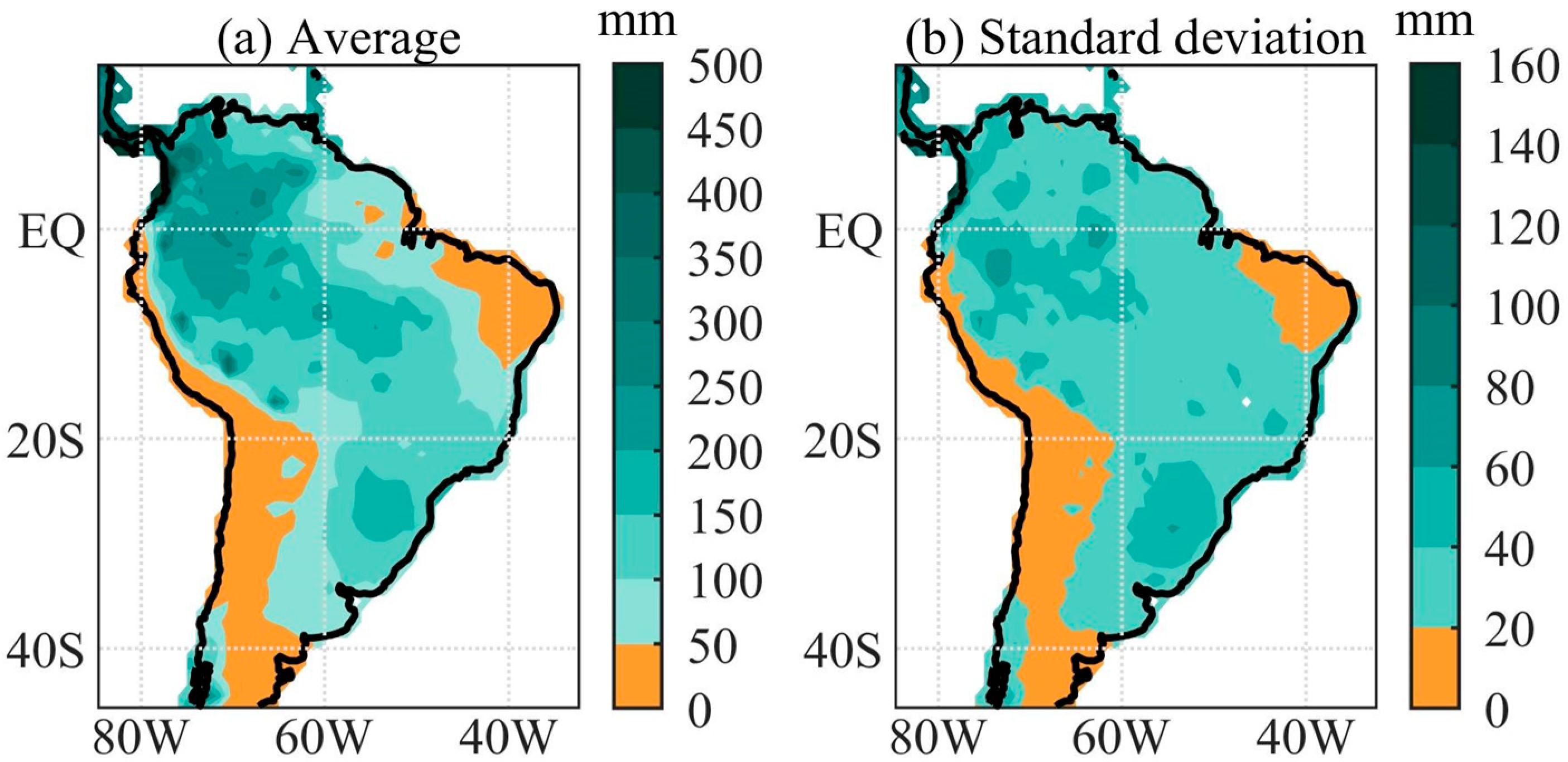
3.1. Austral Spring Rainfall: Climatology and Standard Deviation

Figure 1 discloses the maps of austral spring rainfall climatology and standard deviation. These maps show similar patterns with the lowest averages (less than 50 mm) and standard deviations (less than 20 mm) occurring in almost the same areas, which are along western SA from the equator to central–eastern Argentina and NEB. The largest averages (exceeding 300 mm) were noted in northwestern SA and eastern Amazon, and an average rainfall of between 150 and 200 mm was observed in southern Brazil; standard deviations of between 40 and 60 mm were observed in southern Brazil, northeastern Argentina, northern Uruguay and western Amazonia, and standard deviations above 120 mm were found for the extreme northwestern area of South America (western Colombia).

3.2. EOF Modes of the SST Anomalies in the Tropical Pacific and TIO

Figure 2a depicts the loading pattern of the first EOF mode of the SST anomalies in the tropical Pacific during SON. This mode explained 48% of the interannual austral spring SST variance and was well separated from the other variability modes [41]. For positive PC values, it disclosed the largest positive SST anomalies in the 10° N–10° S band of the central–eastern tropical Pacific (Figure 2a,b). It resembled an SST anomaly pattern previously documented during the developing EN stage [43,44]. The highest positive (negative) values in the first mode PC time series occurred in SON of 1972, 1982, 1987, 1997, and 2009 (1970, 1988, 1995, and 2010) and corresponded to the development of very strong EN (LN) events (Figure 2b). Thus, the PC time series illustrates the interannual variations of the first mode and was used as the ENSO index, referred to as the TPO index.
Figure 2c shows the loading pattern of the first EOF mode of the SST anomalies in the TIO during SON. This mode explained 42% of the interannual SON SST variance, and according to North et al.’s [41] criterium, was well separated from the other modes. It reproduced the SST anomaly features previously described for the positive IOD mode [15]. Indeed, for the positive PC values, this mode disclosed significant positive SST anomalies in the western TIO and the negative ones off the coasts of Java and Sumatra Islands (Figure 2c,d). The PC time series showed interannual oscillations with the highest positive values in the SON of 1972, 1977, 1982, 1997, and 2015, and the equivalent negative values in the SON of 1960, 1964, 1971, 1974, 1975, 1984, 1985, 1996, and 2010 (Figure 2d). The years with the highest positive values coincided with the EN onset years, whereas most years with the highest negative values coincided with the LN onset years (1964, 1971, 1974, 1975, 1984, and 2010). This result confirms previous findings that the positive (negative) IOD and EN (LN) events occur in the same years [20,21]. In some years, the negative IOD (1985 and 1996) events were preceded by LN in the previous year. This result, partway, might reflect the ENSO asymmetry with stronger EN than LN events and longer-lasting LN events than EN events [45]. The significant correlation of 0.74 between the PC time series (Figure 2b,d) of the first EOF variability modes indicates the close relationship between the ENSO and IOD modes. However, this means that ~45% of the TPO and IOD variability modes were totally independent from each other. Then, the R-TPO and R-IOD indices were used to select the corresponding positive and negative events (Table 1).

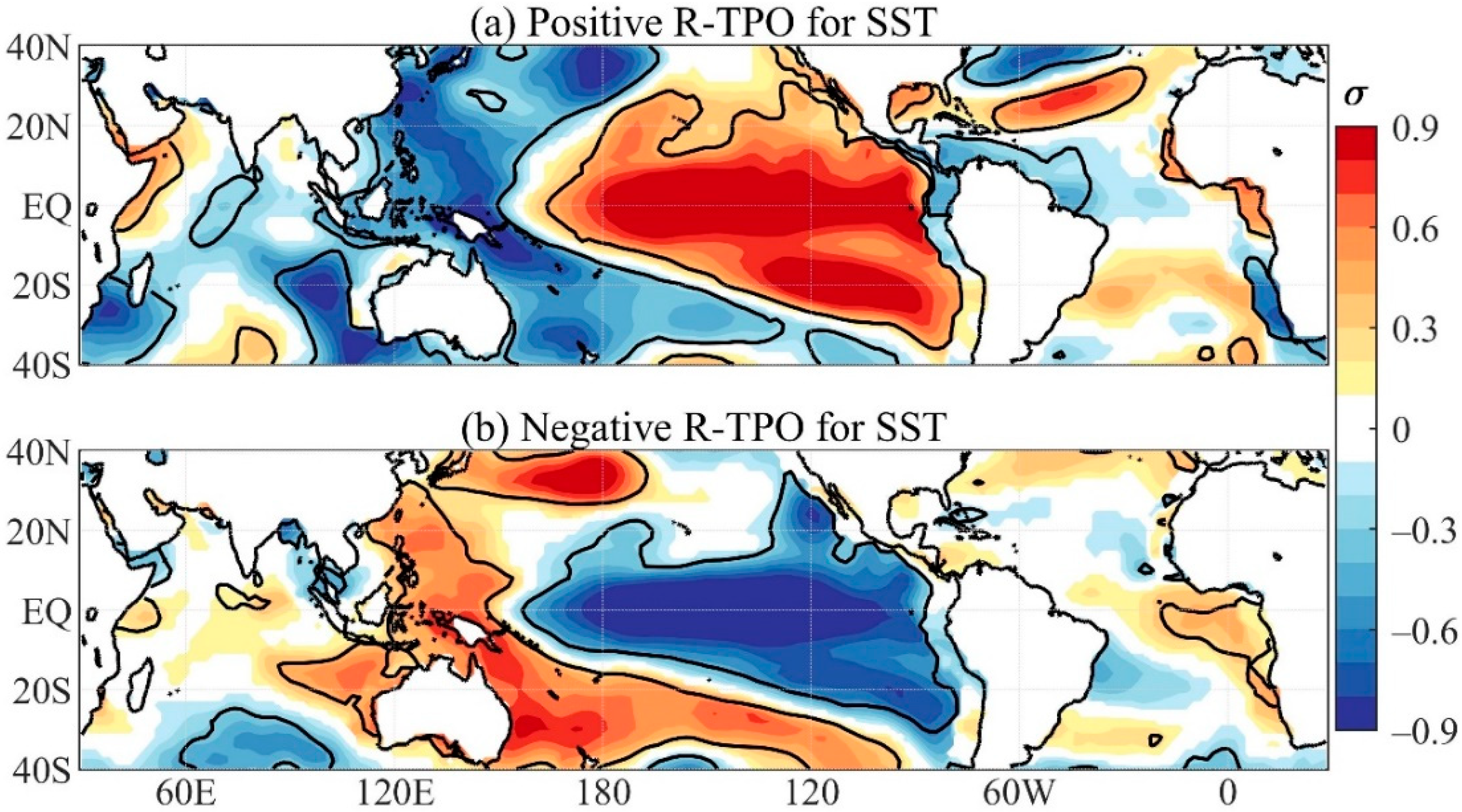
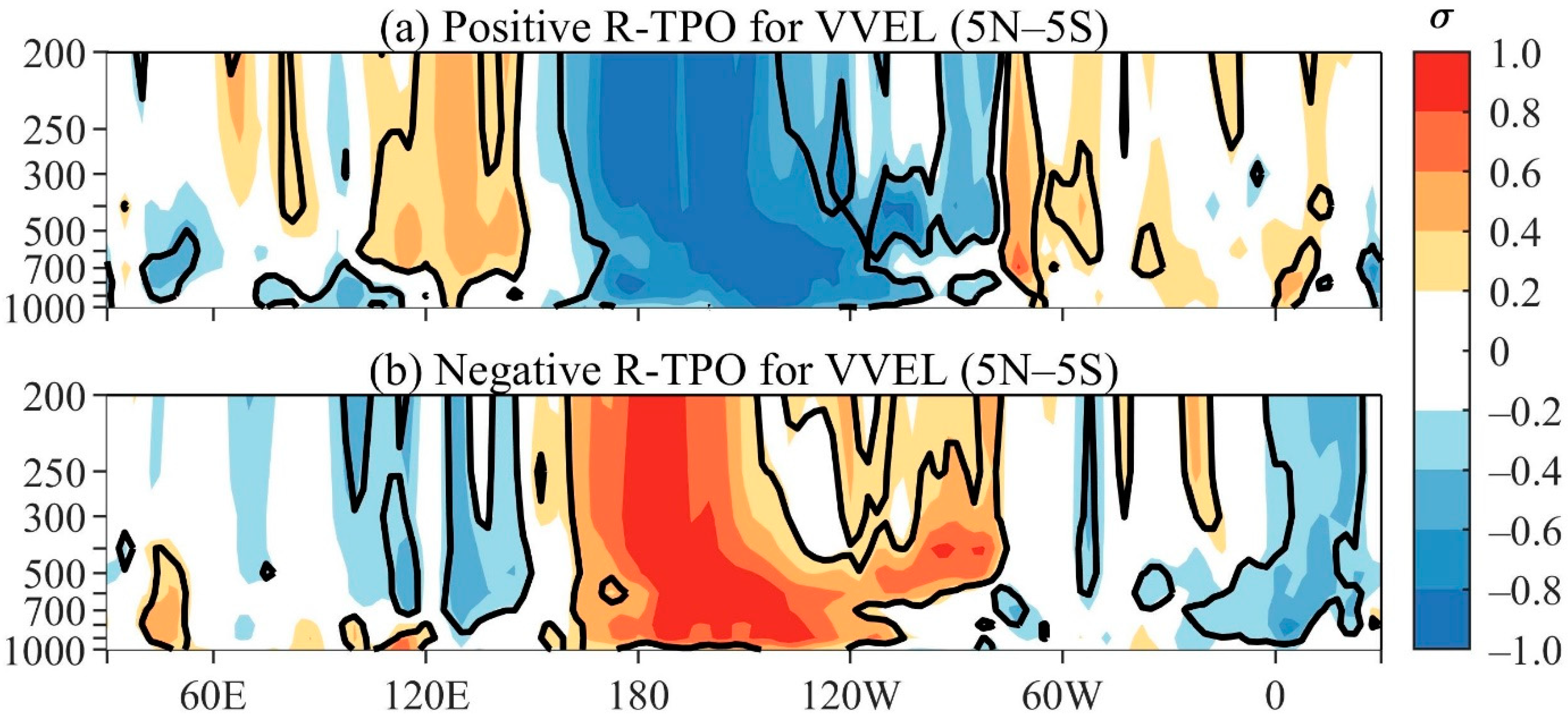
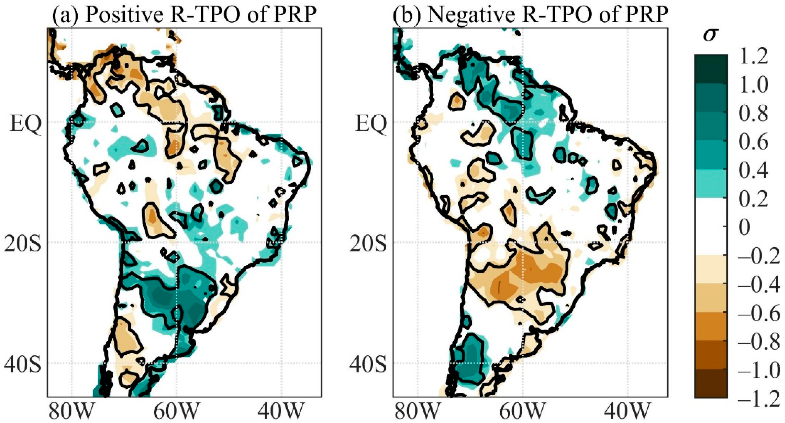
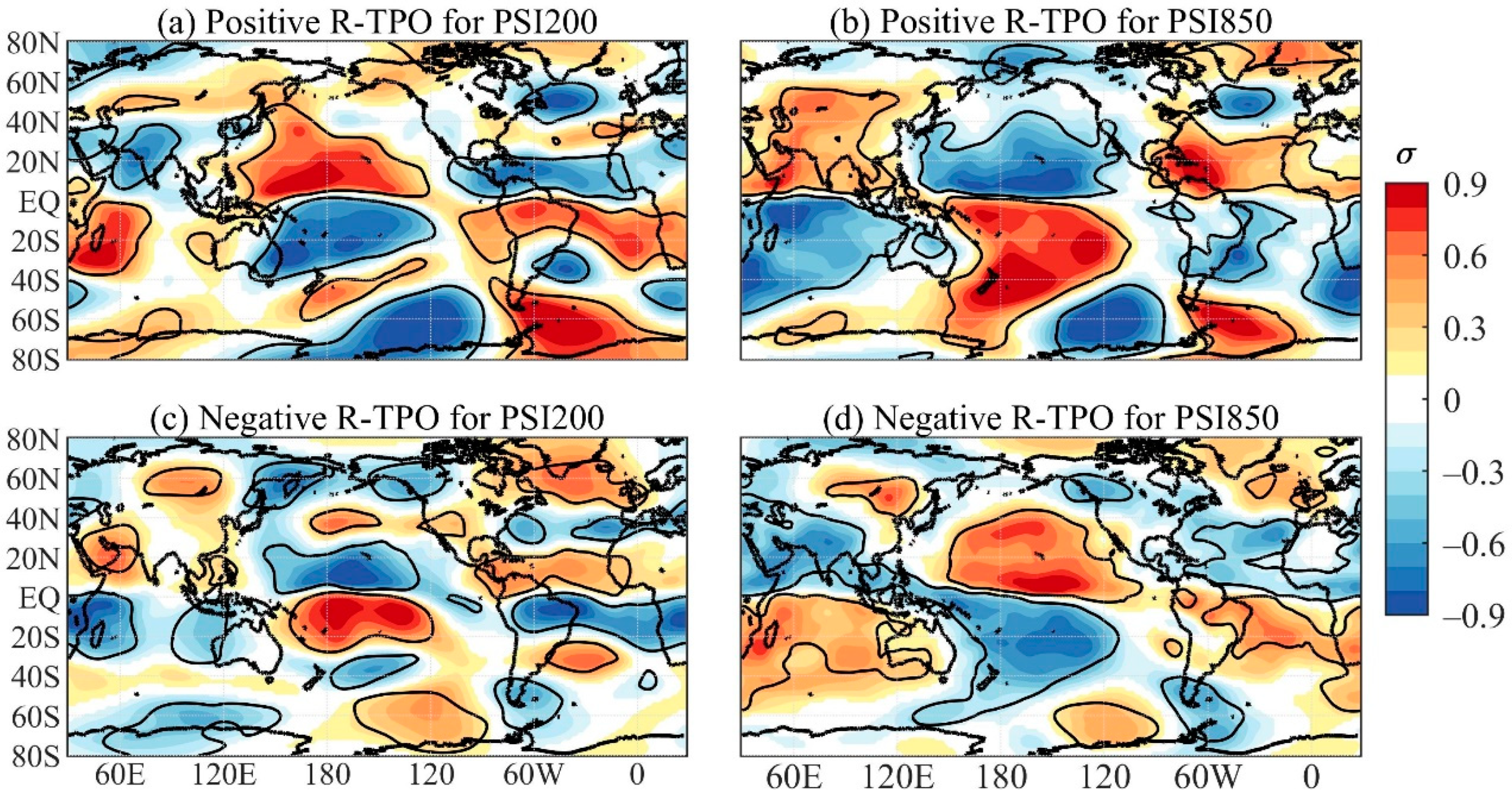
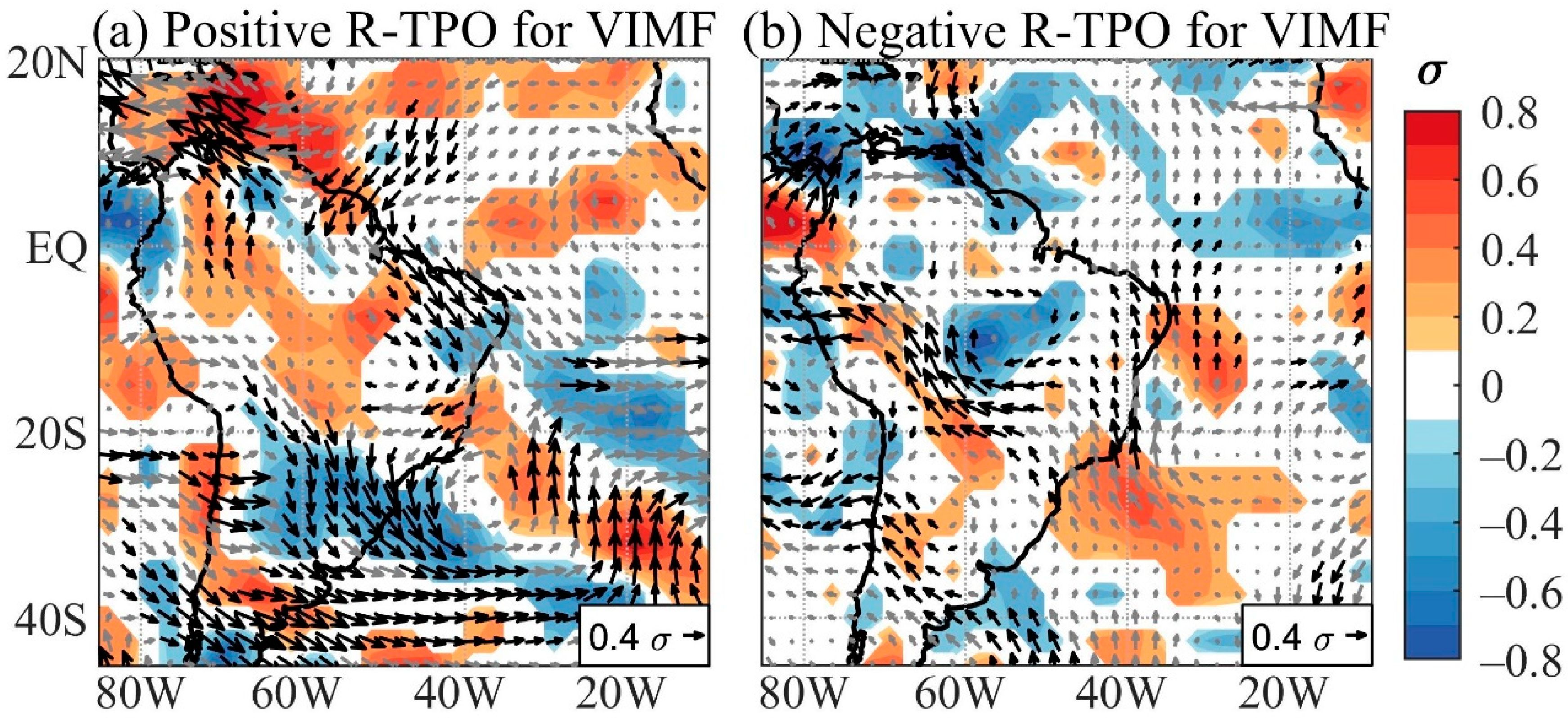
3.3. Residual TPO Composites

The positive and negative R-TPO composites of the residual SST anomalies are disclosed in Figure 3. Both composites featured a prominent pattern with significant opposite sign SST anomalies in the central–eastern tropical Pacific and the equatorial-subtropical western Pacific, significant SST anomalies in small scattered areas in the other tropical Oceans, and no coherent signature of the IOD mode in the TIO (Figure 3a,b). The positive R-TPO composite presented significant positive SST anomalies in the central–eastern tropical Pacific. The positive and negative R-TPO composites featured nearly antisymmetric SST anomaly patterns in the tropical Pacific.
The positive and negative R-TPO composites of residual VVEL anomalies are depicted in longitude vertical cross-sections (Figure 4). Consistent with the corresponding SST anomaly composites (Figure 3a,b), the VVEL anomalies were well-organized along the equatorial Pacific, where the positive and negative R-TPO composites presented nearly antisymmetric patterns (Figure 4a,b). For the positive R-TPO composite, the anomalous Walker cell featured its rising branch over the anomalously warm waters in the central and eastern Pacific (160° E–80° W), and its sinking branch over Indonesia–western Pacific (100° E–150° E) (Figure 3a and Figure 4a). The almost antisymmetric anomalous Walker cell for the negative R-TPO composite disclosed less organized ascending motions in the western side of the 100° E–150° E band (Figure 4b). Additionally, the same sign VVEL anomalies predominantly occurred in the 80° W–30° E band, which were positive for the positive R-TPO composite and negative for the negative R-TPO composite. These anomalies were well-defined, respectively, in the 80° W–40° W and 30° W–30° E bands, thereby without strong antisymmetry in the 80° W–30° E band between the positive and negative R-TPO composites (Figure 4a,b). This feature was particularly noticeable in equatorial SA, where the anomalous sinking motions for the positive R-TPO composite were better organized than the anomalous rising motions for the negative R-TPO composite (Figure 4a,b). In addition, for the positive (negative) R-TPO composite, anomalous rising (sinking) motions were noted in the low to middle tropospheric levels in the 45° E–60° E band (Figure 4a,b).
The positive R-TPO composite of the residual PSI200 (Figure 5a) reflected a Matsuno–Gill-type atmospheric response to the anomalous heating in the eastern tropical Pacific [46,47]. It consisted of pairs of anomalous vortexes in both sides of the equator, which were anticyclones in the central–western Pacific and cyclones in the Indo-Asian and South American–Atlantic–African sectors (Figure 5a). The Pacific–South American (PSA) pattern previously documented for austral summer [2] that connects the western equatorial Pacific and subtropical SA across the Southern Hemisphere (SH) midlatitudes and extratropics was also evident. As part of this pattern, an anomalous anticyclone appeared in the coastal areas of subtropical SA and the surrounding Atlantic (Figure 5a). The corresponding composite of the PSI850 also showed pairs of anomalous vortexes in both sides of the equator, which were better configured and more extensive in the Pacific and African-Indo-Asian regions than in the South American–Atlantic region (Figure 5b). These had a baroclinic structure in the tropics and a nearly equivalent barotropic structure in the subtropics and extratropics. The negative R-TPO composites of the residual PSI200 and PSI850 showed nearly antisymmetric patterns of the corresponding positive R-TPO composites, but the vortexes were slightly weakened and/or their action areas slightly reduced (Figure 5a–d). This feature was particularly noticeable over SA, indicating non-linearity of the R-TPO-associated atmospheric circulations (Figure 5a–d). For the negative R-TPO, it is worth noting an anomalous equivalent barotropic cyclone off the coast of subtropical SA, which was better defined at the upper-level and was part of the Rossby wave train pattern emanating from the central tropical Pacific and following through the SH (Figure 5c,d). Although the SH Rossby wave train pattern was more evident, the Northern Hemisphere (NH) counterpart connecting the equatorial central Pacific and SA was also apparent for both positive and negative R-TPO composites (Figure 5a,c).
The positive R-TPO composite of the residual precipitation presented significant negative anomalies in a northwest–southeast oriented sector extending from Colombia–northwestern Venezuela to southeastern Amazon and in two small areas, one over southeastern Bolivia and the other in central–western SA around 35° S. Moreover, it depicted positive anomalies in a large area, including part of northern and eastern Argentina, most of southern Brazil, and western Uruguay (Figure 6a). The corresponding negative R-TPO composite showed significant positive precipitation anomalies from northwestern Venezuela to central–southern Amazon and in an area over western SA centered at 40° S, and significant negative precipitation anomalies in small, scattered areas of the sector from southeastern Colombia to southern Bolivia and an extensive area mostly west of 55° W, south of 20° S and north of 30° S (Figure 6b). It is worth noting that this latter anomalous dry area was more extensive and located relatively to the north of the anomalous wet area in subtropical SA for the positive R-TPO composite. This result implies that the positive R-TPO and negative R-TPO events affected slightly distinct areas to the south of 20° S.
The positive R-TPO composite of the residual VIMF anomalies featured an anomalous anticyclone over subtropical SA and the surrounding South Atlantic centered at (25° S; 38° W), which transported moisture from central SA and western Amazon into central–southern SA between 20° S and 35° S, where anomalous moisture convergence and positive precipitation anomalies occurred (Figure 6a and Figure 7a). This anticyclone had an equivalent barotropic structure and was part of the SH Rossby wave train pattern associated with anomalous warming in the tropical Pacific (Figure 2a and Figure 5a,b). In addition, anomalous moisture divergence appeared in areas of northwestern SA, central SA between 5° S and 20° S, and a small area in the eastern coast of Brazil (Figure 7a). The moisture divergence in equatorial SA was slightly to the southwest of the area with the largest negative precipitation anomalies (Figure 6a and Figure 7a).
The negative R-TPO composite of the residual VIMF anomalies disclosed an anomalous cyclone in the Atlantic between the equator and 20° S, in whose southwest edge a northwestward flow blew from the subtropical South Atlantic neighboring the area between the southeastern coast of Brazil and Ecuador. The moisture divergence occurred in scattered areas along this flow path where negative precipitation anomalies were noted (Figure 6b and Figure 7b). This cyclone was the remote response, through the Walker cell, to anomalous cooling in the tropical Pacific (Figure 5d). In addition, a cyclone centered over southeastern Amazon induced moisture convergence, which was found to be consistent with positive precipitation anomalies in this area (Figure 6b and Figure 7b).

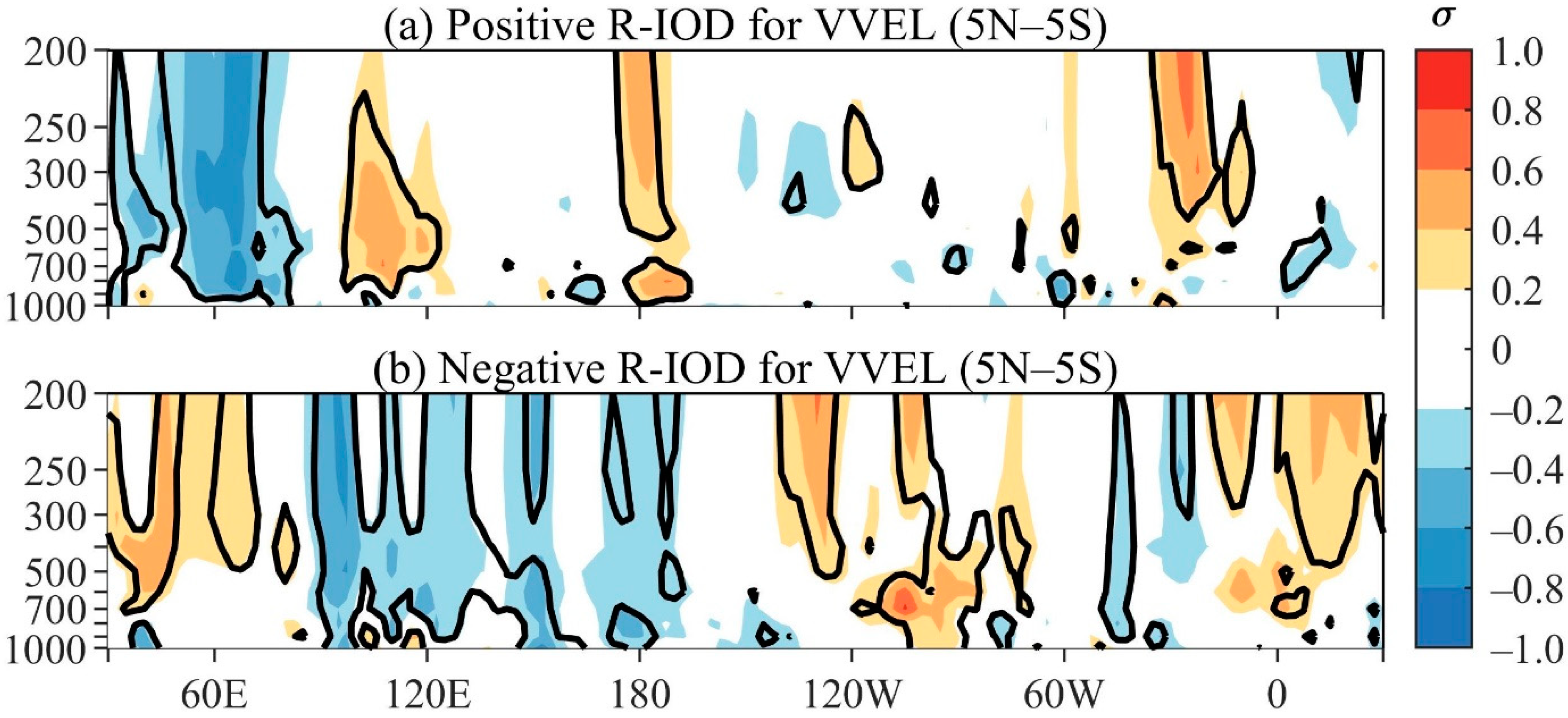
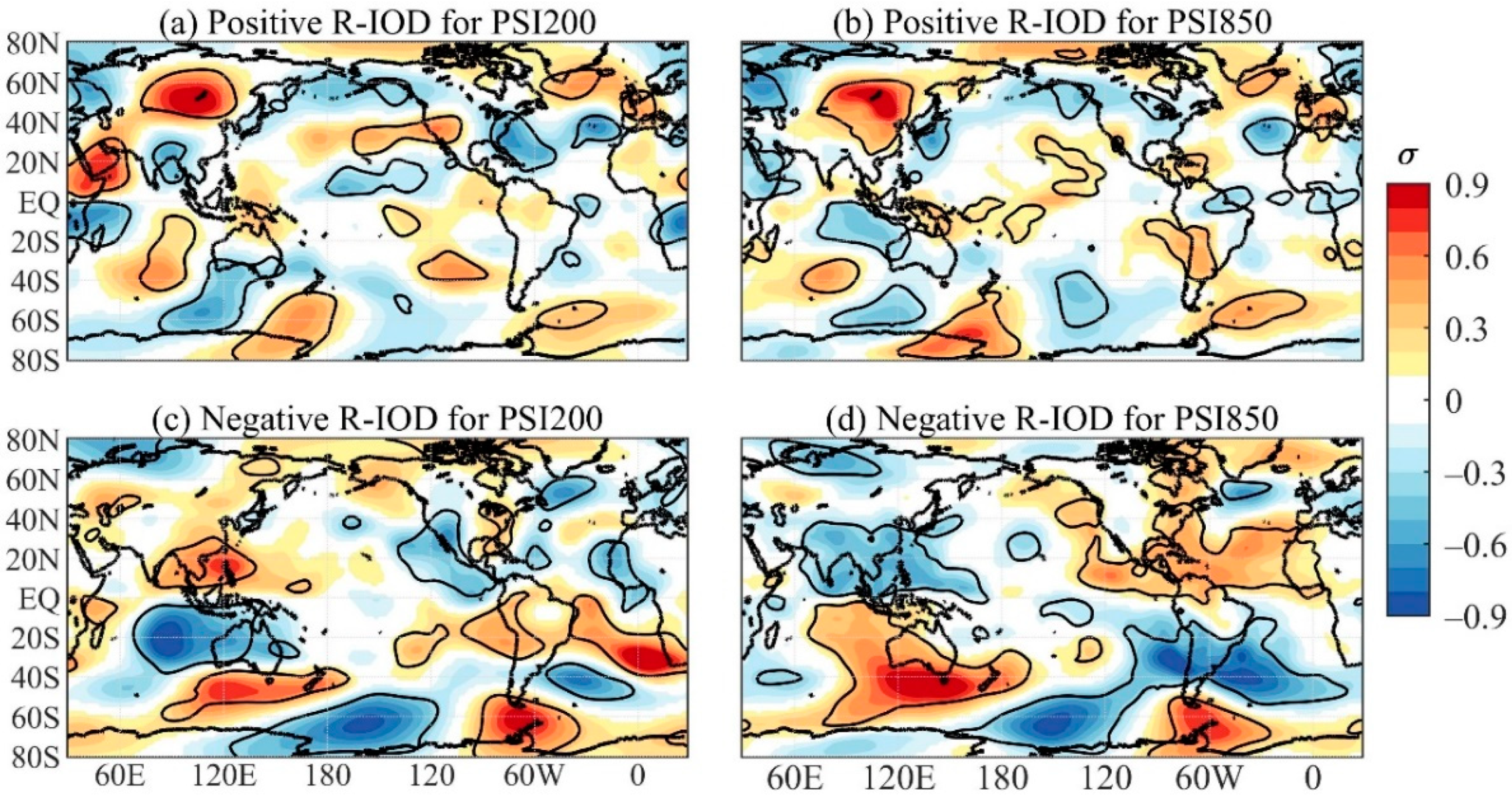
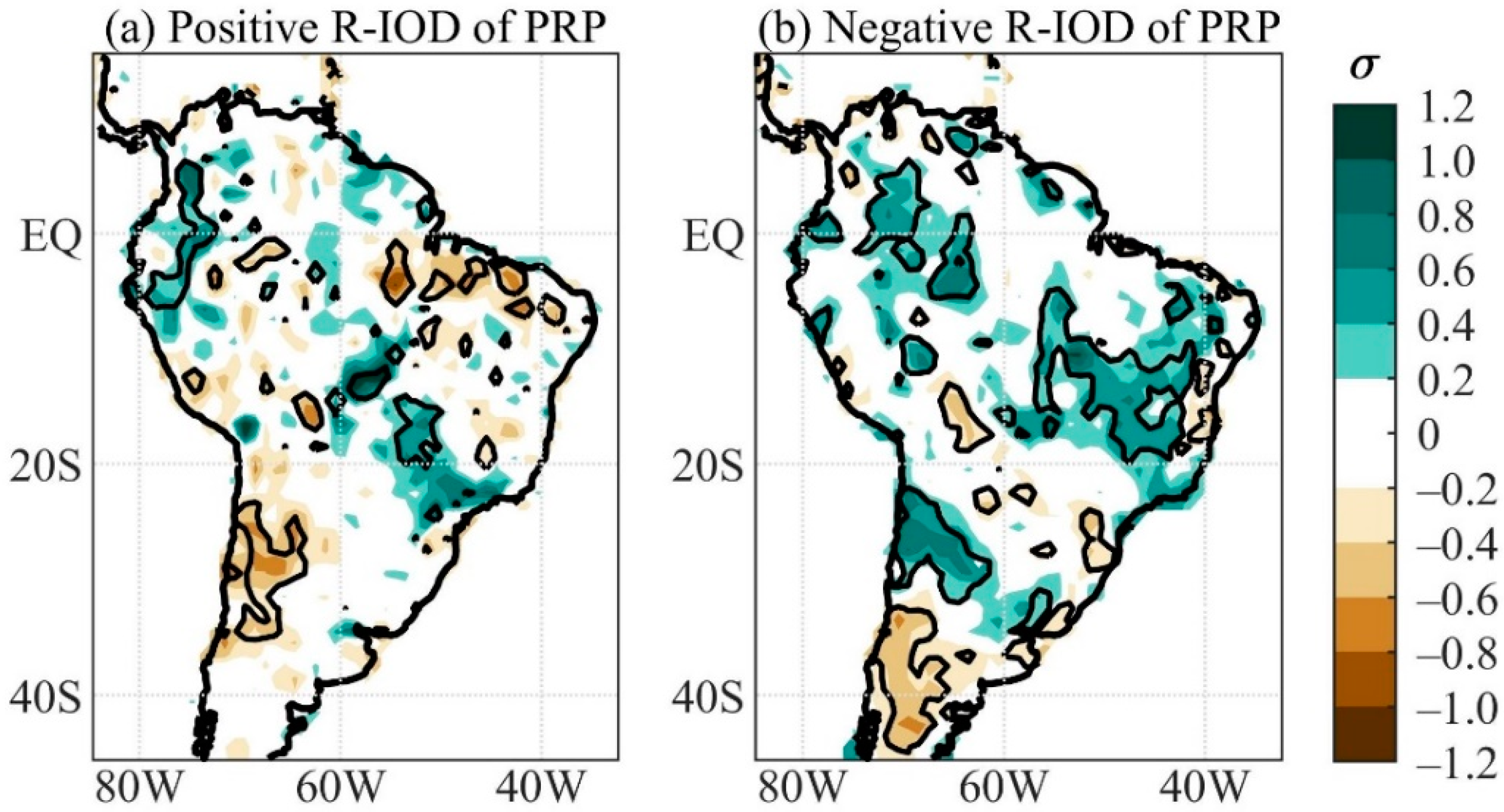
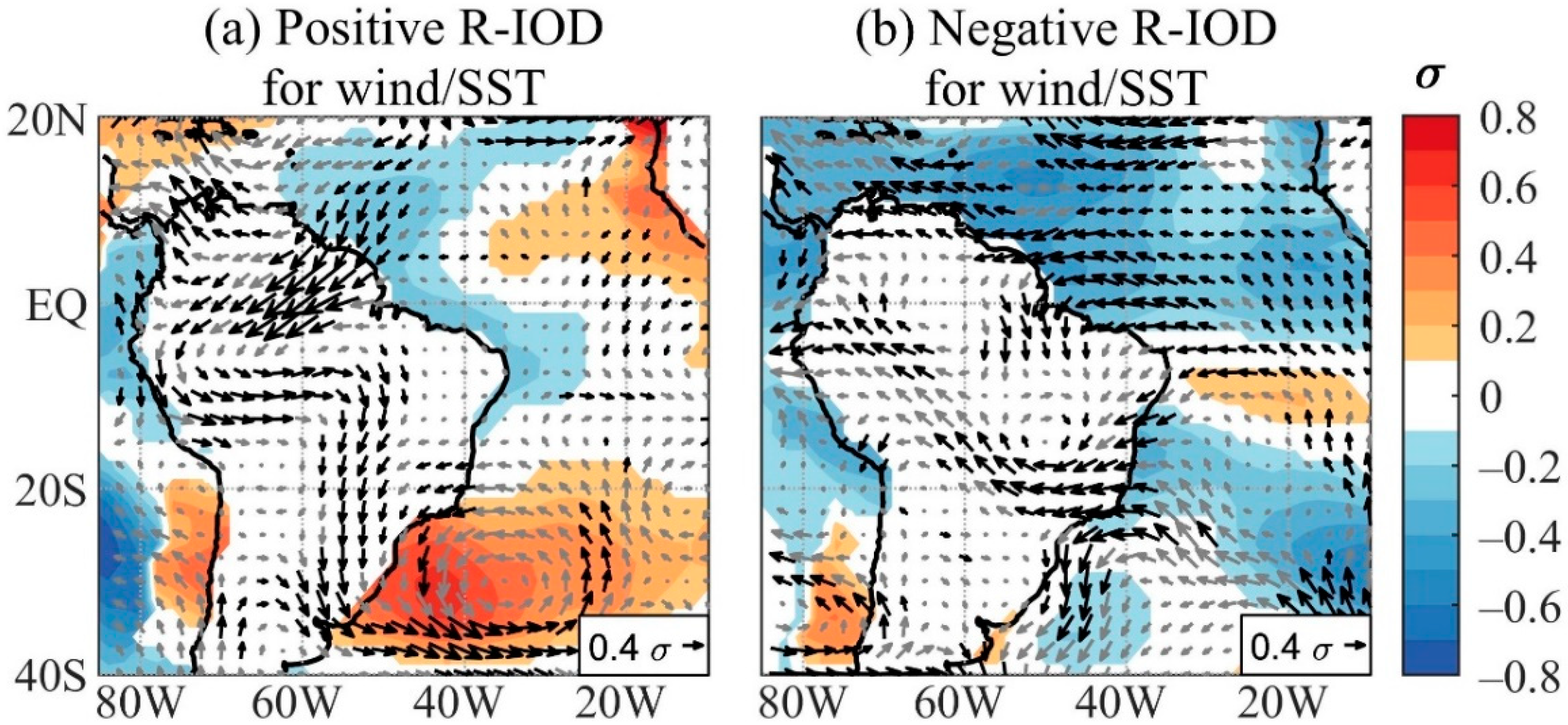
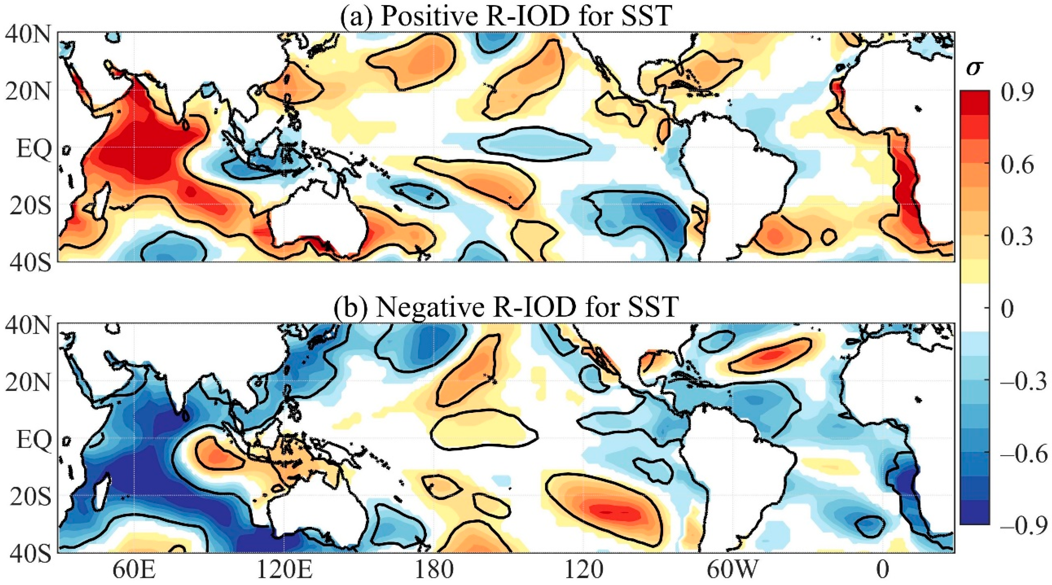
3.4. Residual IOD Composites

Figure 8a,b depict the residual SST anomaly patterns for the positive and negative R-IOD composites, respectively. These patterns showed anomalies of the same sign in an extensive area of TIO, which were positive for the positive R-IOD composite and negative for the negative R-IOD composite, and showed anomalies of the opposite sign off the coasts of Java and Sumatra Islands. These patterns were nearly antisymmetric between the positive and negative R-IOD composites and resembled the positive and negative IOD modes, respectively. For the negative R-IOD composite, pronounced positive SST anomalies were found to the southwest of Sumatra Island (Figure 8b). Outside the TIO, alternating SST anomaly signs occurred in small, scattered areas of the subtropics for positive and negative R-IOD composites. Other areas with significant SST anomalies that deserve to be pointed out included: a negative area along the equatorial Pacific in the 160° W–120° W band for the positive R-IOD composite; a positive area slightly to the north of the equator in the Pacific in the 180° W–130° W band, a negative area in the eastern Pacific approximately between 18° N and 15° S, and a negative area in the western tropical North Atlantic (TNA) south of 20° N for negative R-IOD composite (Figure 8a,b). The SST anomaly patterns for the positive and negative R-IOD composites outside the TIO did not have, in general, tandem correspondences with anomalies of the opposite sign.
The positive and negative R-IOD composites of residual VVEL anomalies are shown in longitude vertical cross-sections along the equator (Figure 9). For the positive R-IOD composite, the VVEL anomalies were well-organized in the TIO longitudes, with anomalous rising and sinking motions, respectively, in the 30° E–85° E and 95° E–120° E bands (Figure 9a). Outside the TIO longitudes, anomalous sinking motions appeared in two narrow bands, one to the east of the dateline, and another in the 30° W–10° W band, with the significant anomalies in this last band limited to the middle and upper tropospheric levels, and very reduced positive VVEL anomalies over the South American longitudes (Figure 9a). For the negative R-IOD composite, significant VVEL anomalies were noted in more extensive bands, with anomalous sinking motions in the middle and upper tropospheric levels of the 15° W–90° E and 150° W–120° W bands and in most tropospheric levels of the 120° W–80° W band, and anomalous rising motions in the 90° E–170° W band and in a narrow band centered at 45° W (Figure 9b). In addition to anomalous rising motions around 45° W, neutral VVEL anomalies predominated in the South American longitudes.
It is worth noting that the largest significant negative VVEL anomalies had a close correspondence with the significant positive SST anomalies along the equatorial western Indian Ocean for the positive R-IOD composite, and in the equatorial eastern Indian Ocean, close to Sumatra coast, for the negative R-IOD composite (Figure 8a,b and Figure 9a,b). For the negative R-IOD composite, although the largest positive SST anomalies manifested to the west of Sumatra Island, positive-to-neutral SST anomalies extended eastward along the equator up to approximately 150° W (Figure 8b). Consistently, the anomalous rising motions extended along the equatorial longitudes from 90° E to 140° E at the most tropospheric levels and from 140° E to 170° W at the low and upper tropospheric levels (Figure 9b).
The positive R-IOD composite of the residual PSI200 anomalies showed a Matsuno–Gill-type atmospheric response to the anomalous heating in the western TIO [46,47] (Figure 10a), consisting of a pair of anomalous anticyclones in both sides of the equator in extreme western TIO and adjacent Africa, and a pair of anomalous cyclones straddling the equator between 20° N and 20° S in the eastern Pacific (180° W–120° W). The outstanding feature was the Rossby wave train pattern induced by the anomalous heating in the western TIO. This pattern emanated from the western TIO, turned southeastward into the Ross Sea, split into two branches around the Amundsen Sea, with one branch turning northeastward to the west of SA and another branch continuing eastward across the Weddell Sea, and induced a weak anomalous anticyclone in the South Atlantic, off the subtropical coast of SA (Figure 10a). The vortexes in the region from the eastern TIO to the southeastern extratropical Pacific presented a meridionally elongated structure. The corresponding composite of the PSI850 did not show a well-configured pair of anomalous vortexes straddling the equator in the Indo-African region; however, the Rossby wave train pattern connecting the western TIO and subtropical SA through the SH was evident (Figure 10b). The PSI850 composite showed an anomalous cyclone over western SA between 20° S and 40° S and the neighboring southeastern Pacific and an anticyclone over eastern Amazon and the surrounding TNA. The positive R-IOD composites of the PSI in both tropospheric levels showed a Rossby wave train pattern connecting TIO and SA through the NH (Figure 10a,b).
The negative R-IOD composite of the residual PSI200 anomalies showed a Matsuno–Gill-type atmospheric response to the anomalous heating in the areas off the coasts of Sumatra and Java Islands [46,47] (Figure 10c), with anomalous vortex couplets, between approximately 35° N and 35° S, straddling the equator; these were anticyclones in the eastern Indo-Asian and western Pacific region, and cyclones in the eastern Pacific and adjacent western SA and Central America. In this case, the most remarkable feature was the Rossby wave train pattern in the SH, whose vortexes were zonally elongated and stronger than those of the positive R-IOD composite (Figure 10a,c). For the negative R-IOD composite, the Rossby wave train pattern extended from the eastern TIO-Indonesian region southeastward into the extratropical southern Pacific Seas, crossed the Bellingshausen Sea, and, in the Weddell Sea, proceeded northeastward into Africa and induced an anticyclone in the South Atlantic centered at (30° W; 40° S) (Figure 10c). The negative R-IOD composite of the residual PSI850 anomalies configured more extensive centers with less horizontal structure than the equivalent composite of residual PSI200 anomalies (Figure 10c,d). Indeed, a pair of low-level anomalous cyclones straddling the equator was noted in the Indo-Asian western Pacific region, with the northern node between the equator and 40° N and the southern node centered to the south of Australia (Figure 10d). Additionally, an anomalous low-level Rossby wave train pattern in the SH was formed by the cyclone to the south of Australia, an anticyclone approximately between the Ross and Amundsen Seas, a cyclone to the south of SA, and, north of this last vortex, a zonally extended anticyclone from eastern Pacific to South Atlantic between 10° S and 50° S (Figure 10d). Finally, an extensive area with low-level anticyclonic circulation was noted in the tropical sector, approximately between the equator and 35° N, extending from the eastern Pacific to the west coast of Africa (Figure 10d).
The vortexes obtained from the composites of the residual PSI200 and PSI850 for the positive R-IOD and negative R-IOD events showed a baroclinic structure in the tropics and a nearly equivalent barotropic structure in the subtropics and extratropics (Figure 10a–d).
The positive R-IOD composite of the residual precipitation anomalies showed significant negative precipitation anomalies in scattered areas along equatorial SA east of 55° W and in subtropical western SA, and showed positive anomalies in a narrow meridional band from western Colombia (south of 7° N) to northern Peru and in scattered areas of central Brazil (Figure 11a). The negative–positive dipole between equatorial SA and central Brazil was further north than that previously presented by Chan et al. [25] for the positive IOD during neutral ENSO years. This difference was due to the distinct data analysis procedures used; in this research, the positive IOD events were selected from R-IOD, and the composites were based on residual precipitation anomalies without the EN effects. For the negative R-IOD composite, significant positive precipitation anomalies predominated in tropical SA, except for small areas in a northwest–southeast oriented band from central–northeastern Bolivia to central–southern Brazil. The largest areas with significant positive anomalies were found in northwestern Amazon, central–eastern Brazil north of 20° S, and western subtropical SA. The largest area with significant negative precipitation anomalies was found in western SA south of 30° S.
The positive R-IOD composite of the residual VIMF and its divergence featured anomalous moisture divergence over the northern coast of Brazil and the adjacent Atlantic, and also in areas of Colombia and northern Peru, and moisture convergence over central–eastern Brazil around 7° S and in southern Brazil, which were associated with an anomalous anticyclone in the South Atlantic centered at (35° W; 30° S) (Figure 12a). The flow associated with this anticyclone in its northern sector extended over the northern coast of Brazil, crossed the Amazon, and then turned southeastward and eastward in northern Peru. It transported moisture into central–eastern and southern Brazil. The moisture divergence–convergence pattern in the northern coast of Brazil and in central–eastern Brazil was consistent with the above-described precipitation anomaly pattern in these areas (Figure 11a and Figure 12a). It is also worth noting that the anticyclone in the subtropical South Atlantic had an equivalent barotropic structure and was part of the Rossby wave train teleconnection patterns connecting the western TIO and SA (Figure 10a). The residual low-level winds showed consistent patterns with those of the VIMF (Figure 12a and Figure 13a). It was, however, noticeable that the low-level divergent area over NEB and in the adjacent equatorial Atlantic justified the moisture divergence in this area (Figure 12a and Figure 13a).
The most outstanding feature of the negative R-IOD composite of the residual VIMF anomalies was a zonally extended anticyclone in the South Atlantic centered at (30° W; 40° S), which was part of SH Rossby wave train pattern associated with the anomalous warming in eastern TIO and the adjacent western Pacific (Figure 10c,d). The flow in the vortex northern edge turned northwestward from the southern coast of Brazil to northern Peru and created areas of moisture divergence along its path, which were coherent with negative precipitation anomalies in these areas (Figure 11b and Figure 12b). Moisture convergence was found in areas north of 20° S of NEB and the surrounding North Atlantic, in central–eastern Brazil, and in small areas of the northern and southwestern Amazon, which were consistent with positive precipitation anomalies (Figure 11b and Figure 12b). Moisture sources seemed to be the subtropical South Atlantic and the TNA, where moisture divergence occurred. This first source connected with the negative R-IOD via the SH Rossby wave train pattern (Figure 10c). The second source seemed to have a more complex relationship with the negative R-IOD, probably through the TIO–equatorial Atlantic connection. A lagged connection existed between the TIO and the equatorial Atlantic via an anomalous Walker cell such that the positive IOD induced Atlantic Niño [48]. This mechanism seemed to occur once the IOD patterns was settled. Here, through an anomalous Walker cell, the negative R-IOD maintained the negative SST in the equatorial Atlantic (Figure 8b) and intensified the easterlies along the Atlantic (longitudes between 20° N and 7° S Figure 13b). Under these conditions, the moisture source remained in the TNA. Additionally, an area of moisture divergence was noted in western SA south of 30° S, which was consistent with negative precipitation anomalies in this same region (Figure 11b and Figure 12b).

4. Discussions and Conclusions

Interannual precipitation variations in SA during austral spring might be modulated by the ENSO [9,10,11] and IOD [25,27] modes. These modes co-exist with simultaneous occurrences of the positive IOD and EN events and negative IOD and LN events [20,21], and they also have close relationships in both directions such that ENSO might induce IOD [31] and vice versa [32]. The relationships between the two modes imply that the IOD-induced climate variability might contain the ENSO effects, and the ENSO-induced climate variability might likewise induce the IOD effects. In addition, there are IOD events that occur during ENSO-neutral years. The effects of this IOD type on South American rainfall during austral spring were previously analyzed [25,27]. Here, the events were selected from the residual indices (R-TPO or R-IOD), and the composites were based on the corresponding residual variables, such that for R-TPO composites, the IOD effects were removed from the variables, and for R-IOD composites, the TPO effects were removed from the variables. Therefore, the present analyses are distinct from those conducted by Chan et al. [25] and Sena and Magnusdottir [27].
The positive R-TPO composite of the residual precipitation featured an anomalous dry–wet rainfall dipole between northern SA (northwest–southeast oriented band from Colombia–northwestern Venezuela to the southeastern Amazon) and part of southeastern SA (northern and eastern Argentina, most of southern Brazil, and western Uruguay) (Figure 6a). The northern dry node was consistent with the sinking motions over equatorial SA that were associated with an anomalous Walker cell (Figure 4a). In addition, the dry–wet dipole was associated with an anomalous equivalent barotropic anticyclone over subtropical SA and the surrounding South Atlantic centered at (25° S; 38° W), which intensified the SALLJ and transported moisture from central SA and western Amazon into central–southern SA between 20° S and 35° S, where anomalous moisture convergence and positive precipitation anomalies occurred (Figure 6a and Figure 7a). These regional atmospheric circulation anomalies were part of the Matsuno–Gill atmospheric response to the anomalous warming in the central and eastern tropical Pacific (Figure 2a) [46,47]. The positive and negative R-TPO composites of the residual precipitation anomalies featured almost antisymmetric patterns in equatorial SA to the north of 7° S, but with the corresponding positive and negative areas to the south of 20° S in slightly distinct positions (Figure 6a,b).
Nevertheless, the nonlinear South American rainfall response to the R-IOD was remarkable (Figure 11a,b). The main reason was that for both positive and negative R-IOD composites, the atmospheric circulation was disturbed by the anomalous heating sources, which were located in the western TIO and off the coasts of Sumatra and Java Islands. The anomalously warmed area in the western TIO was much more extensive than that off the coasts of Sumatra and Java Islands (Figure 8a,b). However, the last anomalously warmed area was contiguous to the maritime continent, where climatologically warm surface waters occur. Thus, the atmospheric circulation anomalies associated with both positive and negative R-IOD composites were strongly driven by the equatorial warmed areas, whose positions were longitudinally distinct between the two composites. These warmed areas induced Matsuno–Gill-type atmospheric responses with distinct associated anomalous Walker cells and Rossby wave train patterns, thus reflecting the nonlinearity of the R-IOD related atmospheric circulation patterns (Figure 9, Figure 10 and Figure 12). Consequently, the R-IOD associated precipitation anomalies presented important nonlinearities. For the positive R-IOD composite, significant precipitation anomalies occurred in small, scattered areas that were negative along equatorial SA east of 55° W and in subtropical western SA, and positive in northwestern SA and central Brazil (Figure 11a). In contrast, for the negative R-IOD composite, significant positive precipitation anomalies predominated in most of tropical SA (Figure 11b).
Comparisons of Figure 1, Figure 6 and Figure 11 indicate that the R-IOD and R-TPO modulated areas with distinct rainfall variabilities. In the equatorial latitudes, the negative R-IOD modulated the areas with the largest rainfall variability in northwestern SA and eastern Amazon, and the negative R-TPO impacted the area with low rainfall variability in northern SA (Figure 1b, Figure 6b and Figure 11b). On the other hand, in the subtropics, both positive and negative R-IOD affected the area with low rainfall variability in western SA, meanwhile both positive and negative R-TPO modulated the area with high rainfall in southern Brazil, northwestern Argentina, and northern Uruguay (Figure 1b, Figure 6 and Figure 11).
The present analysis focuses on austral spring because the IOD is the dominant mode in the TIO during this season, and the canonical EN of Rasmusson and Carpenter’s type [49] peaks in this season. Nevertheless, another EN type, with maximum anomalies in the central Pacific, called Modoki EN [50], reaches its mature stage a few months later than the canonical EN. Several studies have shown that the canonical and Modoki ENSO events have different impacts on South American precipitation [51,52,53]. It is worth recalling that the present analysis does not consider the Modoki ENSO. Therefore, future studies should consider this aspect of the ENSO variability.
One of the most relevant results in this research is the nonlinear precipitation response, that occurred over SA, to the tropical Pacific and TIO forcing when they were considered isolated from each other. Thus, the results from studies using linear approaches such as the EOF or correlation analyses should be taken with caution. The results of the present analysis strongly suggest that monitoring the tropical Indian Ocean during austral spring might be very important for practical purposes.

Author Contributions

Conceptualization—M.T.K., W.L.C. and R.V.A. Methodology—M.T.K., R.V.A. and W.L.C. Software—M.T.K., W.L.C., R.A.F.S. and I.P.S. Validation—M.T.K., R.V.A. and W.L.C. Formal analysis—M.T.K., R.V.A., W.L.C., R.A.F.S., I.P.S. and T.C. Investigation—M.T.K., R.V.A., W.L.C., I.P.S. and T.C. Data curation—M.T.K. and W.L.C. Original draft preparation—M.T.K., R.V.A. and W.L.C. Reviewing and editing—M.T.K., R.V.A., W.L.C., I.P.S., T.C. and R.A.F.S. Visualization—M.T.K. and W.L.C. Supervision—M.T.K. All authors have read and agreed to the published version of the manuscript.

Funding

The Conselho Nacional de Desenvolvimento Científico e Tecnológico (CNPq) of Brazil partially supported the first and third authors under grants 302322/2017-5, and 305611/2019-4, respectively. The second author was partially supported by Project 65146 of the Convocatoria 818 of 2018—Colciencias, IC-21106 from the Universidad del Valle (Cali-Colombia). Support for the National Centers for Environmental Prediction/National Center for Atmospheric Research (NCEP/NCAR) Reanalysis-I Project dataset was provided by the National Oceanic and Atmospheric Administration/Earth System Research Laboratories/Physical Sciences Laboratory (NOAA/ESRL/PSL). Support for the extended reconstructed SST version V5 dataset and for the precipitation GPCC dataset was provided by NOAA/ESRL/PSL. The authors thank the two anonymous reviewers for their helpful comments.

Institutional Review Board Statement

Not applicable.

Informed Consent Statement

Not applicable.

Data Availability Statement

Not applicable.

Conflicts of Interest

The authors declare no conflict of interest. The founding sponsors had no role in the design, analysis, and interpretation of data, in the writing manuscript, or in the decision to publish the results.

References

  1. Zhou, J.; Lau, K.M. Principal modes of interannual and decadal variability of summer rainfall over South America. Int. J. Climatol. 2001, 21, 1623–1644. [Google Scholar] [CrossRef]
  2. Mo, K.C.; Higgins, R.W. The Pacific-South American modes and tropical convection during the Southern Hemisphere winter. Mon. Weather Rev. 1998, 126, 1581–1596. [Google Scholar] [CrossRef]
  3. Paegle, J.N.; Mo, K.C. Linkages between summer rainfall variability over South America and sea surface temperature anomalies. J. Clim. 2002, 15, 1389–1407. [Google Scholar] [CrossRef] [Green Version]
  4. Ropelewski, C.F.; Halpert, M.S. Global and Regional scale precipitation patterns associated with the El Niño-Southern Oscillation. Mon. Weather Rev. 1987, 115, 1606–1626. [Google Scholar] [CrossRef] [Green Version]
  5. Kousky, V.E.; Ropelewski, C.F. Extremes in the Southern Oscillation and their Relationship to Precipitation Anomalies with Emphasis on the South American Region. Rev. Bras. Meteorol. 1989, 4, 351–363. [Google Scholar]
  6. Aceituno, P. On the Functioning of the Southern Oscillation in the South American Sector. Part I: Surface Climate. Mon. Weather Rev. 1988, 116, 505–524. [Google Scholar] [CrossRef] [Green Version]
  7. Kayano, M.T.; Rao, V.B.; Moura, A.D. Tropical circulations and the associated rainfall anomalies during two contrasting years. J. Climatol. 1988, 8, 477–488. [Google Scholar] [CrossRef] [Green Version]
  8. Rao, V.B.; Hada, K. Characteristics of rainfall over Brazil: Annual variations and connections with the Southern Oscillation. Theor. Appl. Climatol. 1990, 42, 81–91. [Google Scholar] [CrossRef]
  9. Grimm, A.M. Interannual climate variability in South America: Impacts on seasonal precipitation, extreme events, and possible effects of climate change. Stoch. Environ. Res. Risk Assess. 2011, 25, 537–554. [Google Scholar] [CrossRef]
  10. Grimm, A.M.; Zilli, M.T. Interannual variability and seasonal evolution of summer monsoon rainfall in South America. J. Clim. 2009, 22, 2257–2275. [Google Scholar] [CrossRef]
  11. De Souza, I.P.; Andreoli, R.V.; Kayano, M.T.; Vargas, F.F.; Cerón, W.L.; Martins, J.A.; Freitas, E.; de Souza, R.A.F. Seasonal precipitation variability modes over South America associated to El Niño-Southern Oscillation (ENSO) and non-ENSO components during the 1951–2016 period. Int. J. Climatol. 2021, 41, 4321–4338. [Google Scholar] [CrossRef]
  12. Grimm, A.M.; Ferraz, S.E.T.; Gomes, J. Precipitation Anomalies in Southern Brazil Associated with El Niño and La Niña Events. J. Clim. 1998, 11, 2863–2880. [Google Scholar] [CrossRef] [Green Version]
  13. Taschetto, A.S.; Ambrizzi, T. Can Indian Ocean SST anomalies influence South American rainfall? Clim. Dyn. 2012, 38, 1615–1628. [Google Scholar] [CrossRef] [Green Version]
  14. Kayano, M.T.; Andreoli, R.V.; Cerón, W.L.; Souza, R.A.F. The Role of the Indian Ocean Basin-Wide and El Niño—Southern Oscillation Modes in Interannual Rainfall Variability over South America during Austral Summer. Atmosphere 2021, 12, 1094. [Google Scholar] [CrossRef]
  15. Saji, N.H.; Goswani, B.N.; Vinayachandran, P.N.; Yamagat, T. A dipole mode in the tropical Indian Ocean. Nature 1999, 401, 360–363. [Google Scholar] [CrossRef] [PubMed]
  16. Klein, S.A.; Soden, B.J.; Lau, N.-C. Remote Sea Surface Temperature Variations during ENSO: Evidence for a Tropical Atmospheric Bridge. J. Clim. 1999, 12, 917–932. [Google Scholar] [CrossRef] [Green Version]
  17. Deser, C.; Alexander, M.A.; Xie, S.P.; Phillips, A.S. Sea surface temperature variability: Patterns and mechanisms. Annu. Rev. Mar. Sci. 2010, 2, 115–143. [Google Scholar] [CrossRef] [PubMed] [Green Version]
  18. Lim, E.P.; Hendon, H.H. Causes and Predictability of the Negative Indian Ocean Dipole and Its Impact on la Niña during 2016. Sci. Rep. 2017, 7, 1–11. [Google Scholar] [CrossRef] [Green Version]
  19. Lau, N.C.; Nath, M.J. Atmosphere-ocean variations in the Indo-Pacific sector during ENSO episodes. J. Clim. 2003, 16, 3–20. [Google Scholar] [CrossRef]
  20. Wang, X.; Wang, C. Different impacts of various El Niño events on the Indian Ocean Dipole. Clim. Dyn. 2014, 42, 991–1005. [Google Scholar] [CrossRef]
  21. Sun, S.; Lan, J.; Yue Fang, T.; Gao, X. A triggering mechanism for the Indian Ocean dipoles independent of ENSO. J. Clim. 2015, 28, 5063–5076. [Google Scholar] [CrossRef]
  22. Webster, P.J.; Moore, A.M.; Loschnigg, J.P.; Leben, R.R. Coupled ocean-atmosphere dynamics in the Indian Ocean during 1997–98. Nature 1999, 401, 356–360. [Google Scholar] [CrossRef] [PubMed]
  23. Annamalai, H.; Xie, S.P.; McCreary, J.P.; Murtugudde, R. Impact of Indian Ocean Sea surface temperature on developing El Niño. J. Clim. 2005, 18, 302–320. [Google Scholar] [CrossRef]
  24. Xie, S.P.; Hu, K.; Hafner, J.; Tokinaga, H.; Du, Y.; Huang, G.; Sampe, T. Indian Ocean capacitor effect on Indo-Western pacific climate during the summer following El Niño. J. Clim. 2009, 22, 730–747. [Google Scholar] [CrossRef]
  25. Chan, S.C.; Behera, S.K.; Yamagata, T. Indian Ocean Dipole influence on South American rainfall. Geophys. Res. Lett. 2008, 35, 10–14. [Google Scholar] [CrossRef]
  26. Saji, N.H.; Ambrizzi, T.; Ferraz, S.E.T. Indian Ocean Dipole mode events and austral surface air temperature anomalies. Dyn. Atmos. Ocean. 2005, 39, 87–101. [Google Scholar] [CrossRef]
  27. Sena, A.C.T.; Magnusdottir, G. Influence of the Indian Ocean dipole on the large-scale circulation in South America. J. Clim. 2021, 34, 6057–6068. [Google Scholar]
  28. Wang, H.; Murtugudde, R.; Kumar, A. Evolution of Indian Ocean dipole and its forcing mechanisms in the absence of ENSO. Clim. Dyn. 2016, 47, 2481–2500. [Google Scholar] [CrossRef]
  29. Yamagata, T.; Behera, S.K.; Luo, J.J.; Masson, S.; Jury, M.R.; Rao, S.A. Coupled ocean-atmosphere variability in the tropical Indian Ocean. Geophys. Monogr. Ser. 2004, 147, 189–211. [Google Scholar]
  30. Golden Gate Weather Service El Niño and La Niña Years and Intensities. Based on Oceanic Niño Index (ONI). Available online: https://ggweather.com/enso/oni.htm (accessed on 1 September 2021).
  31. Zhao, Y.; Nigam, S. The Indian Ocean dipole: A monopole in SST. J. Clim. 2015, 28, 3–19. [Google Scholar] [CrossRef] [Green Version]
  32. Wang, C. Three-ocean interactions and climate variability: A review and perspective. Clim. Dyn. 2019, 53, 5119–5136. [Google Scholar] [CrossRef] [Green Version]
  33. Huang, B.; Thorne, P.W.; Banzon, V.F.; Boyer, T.; Chepurin, G.; Lawrimore, J.H.; Menne, M.J.; Smith, T.M.; Vose, R.S.; Zhang, H.M. Extended reconstructed Sea surface temperature, Version 5 (ERSSTv5): Upgrades, validations, and intercomparisons. J. Clim. 2017, 30, 8179–8205. [Google Scholar] [CrossRef]
  34. National Oceanic and Atmospheric Administration; Extended Reconstructed Sea Surface Temperature (NOAA/ERSST) SST data. Available online: https://www.esrl.noaa.gov/psd/data/gridded/ (accessed on 1 March 2018).
  35. Schneider, U.; Becker, A.; Finger, P.; Meyer-Christoffer, A.; Ziese, M.; Rudolf, B. GPCC’s new land surface precipitation climatology based on quality-controlled in situ data and its role in quantifying the global water cycle. Theor. Appl. Climatol. 2014, 115, 15–40. [Google Scholar] [CrossRef] [Green Version]
  36. Global Precipitation Climatology Centre (GPCC) Monthly Gridded Precipitation Data. Available online: https://www.esrl.noaa.gov/psd/data/gridded/data.gpcc.html (accessed on 3 May 2019).
  37. Kalnay, E.; Kanamitsu, M.; Kistler, R.; Collins, W.; Deaven, D.; Gandin, L.; Iredell, M.; Saha, S.; White, G.; Woollen, J.; et al. The NCEP/NCAR reanalysis project. Bull. Am. Meteorol. Soc. 1996, 77, 437–471. [Google Scholar] [CrossRef] [Green Version]
  38. National Center for Environmental Prediction; National Center for Atmospheric Research (NCEP/NCAR) Reanalysis-I Project Dataset. Available online: https://psl.noaa.gov/data/gridded/ (accessed on 3 September 2020).
  39. Peixoto, J.P.; Oort, A.H. Physics of Climate; MIT Press: San Diego, CA, USA, 1992; ISBN 7287064. [Google Scholar]
  40. Torrence, C.; Compo, G.P. A Practical Guide to Wavelet Analysis Christopher. Bull. Am. Meteorol. Soc. 1998, 97, 61–78. [Google Scholar] [CrossRef] [Green Version]
  41. North, G.L.; Bell, T.L.; Chalan, R.F. Sampling Errors in the Estimation of Empirical Othogonal Functions. Mon. Weather Rev. 1982, 110, 699–706. [Google Scholar] [CrossRef]
  42. Panofsky, H.G.; Brier, G.W. Some Applications of Statistics to Meteorology; Pennsylvania State University: Pennsylvania, PA, USA, 1968. [Google Scholar]
  43. Rasmusson, E.M.; Wallace, J.M. Meteorological Aspects of the El Niño/Southern Oscillation. Science 1983, 222, 1195–1202. [Google Scholar] [CrossRef]
  44. Rasmusson, E.M.; Arkin, P.A. Interannual climate variability associated with the El Niño/Southern Oscillation. Elsevier Oceanogr. Ser. 1985, 40, 697–725. [Google Scholar]
  45. An, S.I.; Jin, F.F. Nonlinearity and asymmetry of ENSO. J. Clim. 2004, 17, 2399–2412. [Google Scholar] [CrossRef]
  46. Matsuno, T. Quasi-Geostrophic Motions in the Equatorial Area. J. Meteorol. Soc. Jpn. Ser. II 1966, 44, 25–43. [Google Scholar] [CrossRef] [Green Version]
  47. Gill, A.E. Some simple solutions for heat-induced tropical circulation. Q. J. R. Meteorol. Soc. 1980, 106, 447–462. [Google Scholar] [CrossRef]
  48. Liao, H.; Wang, C. Sea Surface Temperature Anomalies in the Western Indian Ocean as a Trigger for Atlantic Niño Events. Geophys. Res. Lett. 2021, 48, e2021GL092489. [Google Scholar] [CrossRef]
  49. Rasmusson, E.M.; Carpenter, T.H. Variation in tropical sea surface temperature and surface wind fields associated with Southern Oscillation/El Niño. Mon. Weather Rev. 1982, 110, 354–384. [Google Scholar] [CrossRef]
  50. Ashok, K.; Behera, S.K.; Rao, S.A.; Weng, H.; Yamagata, T. El Niño Modoki and its possible teleconnection. J. Geophys. Res. Ocean. 2007, 112, 1–27. [Google Scholar] [CrossRef]
  51. Tedeschi, R.G.; Cavalcanti, I.F.A.; Grimm, A.M. Influences of two types of ENSO on South American precipitation. Int. J. Climatol. 2013, 33, 1382–1400. [Google Scholar] [CrossRef]
  52. Andreoli, R.V.; de Oliveira, S.S.; Kayano, M.T.; Viegas, J.; de Souza, R.A.F.; Candido, L.A. The influence of different El Niño types on the South American rainfall. Int. J. Climatol. 2017, 37, 1374–1390. [Google Scholar] [CrossRef]
  53. Andreoli, R.V.; Kayano, M.T.; Viegas, J.; de Oliveira, S.S.; de Souza, R.A.F.; Garcia, S.R.; Rego, W.H.T.; de Oliveira, M.B.L. Effects of two different La Niña types on the South American rainfall. Int. J. Climatol. 2019, 39, 1415–1428. [Google Scholar] [CrossRef]
Figure 1. Austral spring rainfall: (a) climatology (mm); and (b) standard deviation (mm).
Atmosphere 12 01437 g001
Figure 2. Spatial loading pattern and principal component (PC) time series of first EOF mode the interannual SST anomalies during the southern springs of the 1951–2016 period for the: (a) tropical Pacific Ocean; (b) PC for the tropical Pacific loading pattern; (c) tropical Indian Ocean; and (d) PC for the tropical Indian Ocean loading pattern. Continuous contours encompass the significant correlations at a 95% confidence level using the Student’s t-test.
Atmosphere 12 01437 g002
Figure 3. Composite of the residual SST anomalies during austral spring for the: (a) positive R-TPO; and (b) negative R-TPO. In this Figure, residual means without the IOD effects. Continuous contours encompass significant values at a 95% confidence level using the Student’s t-test.
Atmosphere 12 01437 g003
Figure 4. Longitude vertical cross-sections of the composites of the residual VVEL anomalies during austral spring for the: (a) positive R-TPO; and (b) negative R-TPO. In this Figure, residual means without the IOD effects. Continuous contours encompass significant values at a 95% confidence level using the Student’s t-test. The vertical pressure levels are in hPa.
Atmosphere 12 01437 g004
Figure 5. Composites of the residual zonally asymmetric streamfunction anomalies during austral spring for the: (a) positive R-TPO and PSI200; (b) positive R-TPO and PSI850; (c) negative R-TPO and PSI200; and (d) negative R-TPO and PSI850. In this Figure, residual means without the IOD effects. Continuous contours encompass significant values at a 95% confidence level using the Student’s t-test.
Atmosphere 12 01437 g005
Figure 6. Composites of the residual precipitation anomalies during austral spring for the: (a) positive R-TPO; (b) negative R-TPO. In this Figure, residual means without the IOD effects. Continuous contours encompass significant values at a 95% confidence level using the Student’s t-test.
Atmosphere 12 01437 g006
Figure 7. Composites of the anomalies of the residual VIMF components and of their divergence (shades) during austral spring for the: (a) positive R-TPO; and (b) negative R-TPO. In this Figure, residual means without the IOD effects. Shades encompass significant values at a 95% confidence level using the Student’s t-test. Vectors indicate the VIMF components. The arrow in the right-lower corner gives the vector base magnitude in S.D. units. Bold arrows indicate vectors when at least one component has a significant 95% confidence level value.
Atmosphere 12 01437 g007
Figure 8. Composite of the residual SST anomalies during austral spring for the: (a) positive R-IOD; and (b) negative R-IOD. In this Figure, residual means without the TPO effects. Graphical display is the same as that in Figure 3.
Atmosphere 12 01437 g008
Figure 9. Longitude vertical cross-sections of the composites of the residual VVEL anomalies during austral spring for the: (a) positive R-IOD; and (b) negative R-IOD. In this Figure, residual means without the TPO effects. Graphical display is the same as that in Figure 4.
Atmosphere 12 01437 g009
Figure 10. Composites of the residual zonally asymmetric streamfunction anomalies during austral spring for the: (a) positive R-IOD and PSI200; (b) positive R-IOD and PSI850; (c) negative R-IOD and PSI200; and (d) negative R-IOD and PSI850. In this Figure, residual means without the TPO effects. Graphical display is the same as that in Figure 5.
Atmosphere 12 01437 g010
Figure 11. Composites of the residual precipitation anomalies during austral spring for the: (a) positive R-IOD; (b) negative R-IOD. In this Figure, residual means without the TPO effects. Graphical display is the same as that in Figure 6.
Atmosphere 12 01437 g011
Figure 12. Composites of the anomalies of the residual VIMF components and of their divergence (shades) during austral spring for the: (a) positive R-IOD; and (b) negative R-IOD. In this Figure, residual means without the TPO effects. Graphical display is the same as that in Figure 7.
Atmosphere 12 01437 g012
Figure 13. Composites of the anomalies of the residual 850hPa winds and SST (shades) during austral spring for the: (a) positive R-IOD; and (b) negative R-IOD. Shades encompass significant values at a 95% confidence level using the Student’s t-test. In this Figure, residual means without the TPO effects. The arrow in the right-lower corner gives the vector base magnitude in S.D. units. Bold arrows indicate vectors when at least one component has a significant 95% confidence level value.
Atmosphere 12 01437 g013
Table 1. Selected years of the positive and negative R-TPO and R-IOD events.
Positive R-TPO1965, 1968, 1971, 1986, 1997, 2009, 2010
Negative R-TPO1955, 1967, 1973, 1988, 1995, 2007, 2016
Positive R-IOD1967, 1973, 1977, 1983, 1988, 1995, 2007
Negative R-IOD1960, 1965, 1968, 1971, 1986, 1996, 2009
Publisher’s Note: MDPI stays neutral with regard to jurisdictional claims in published maps and institutional affiliations.

