Comparative Analysis of Predictive Models for Fine Particulate Matter in Daejeon, South Korea


Abstract
:1. Introduction
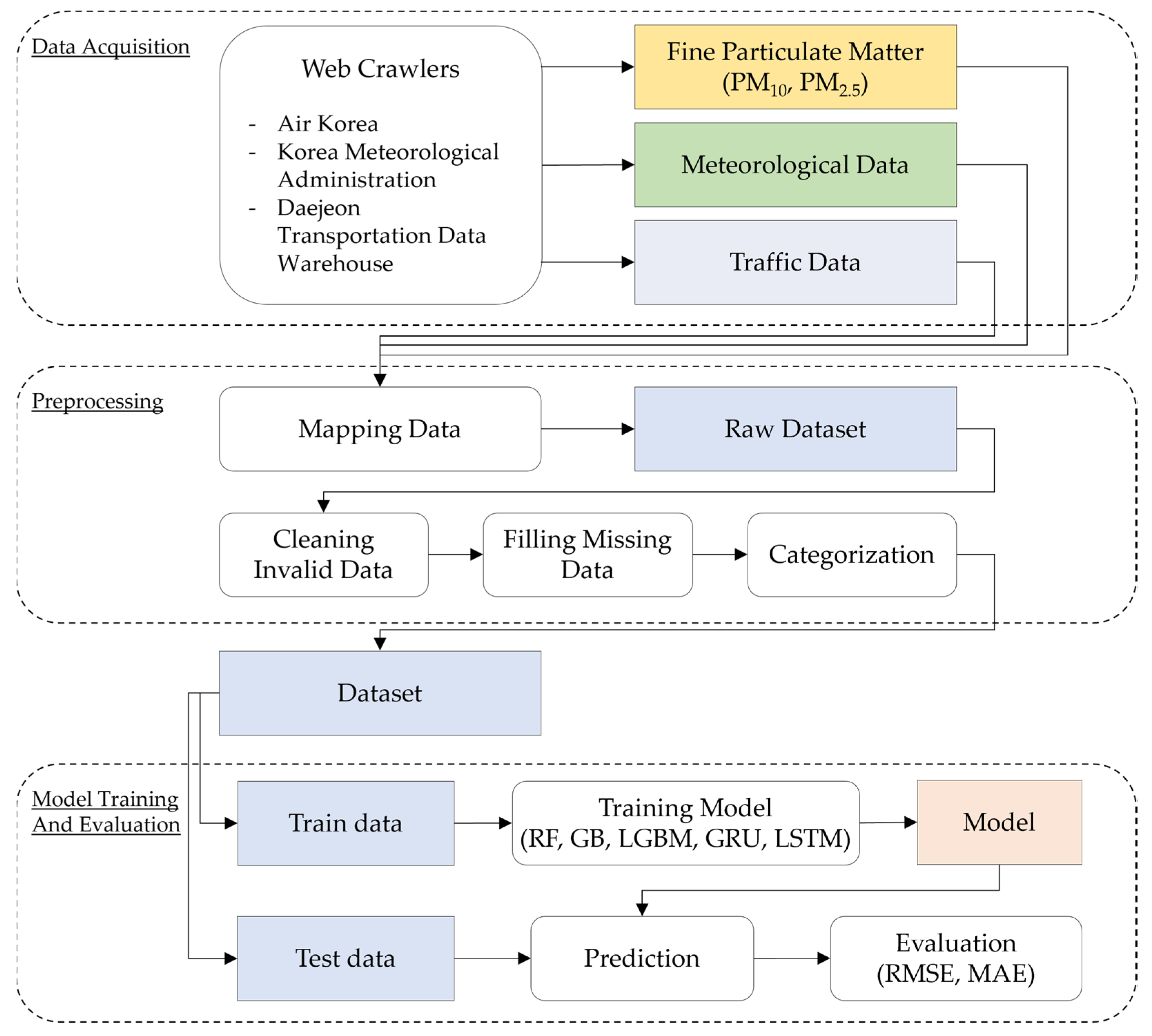
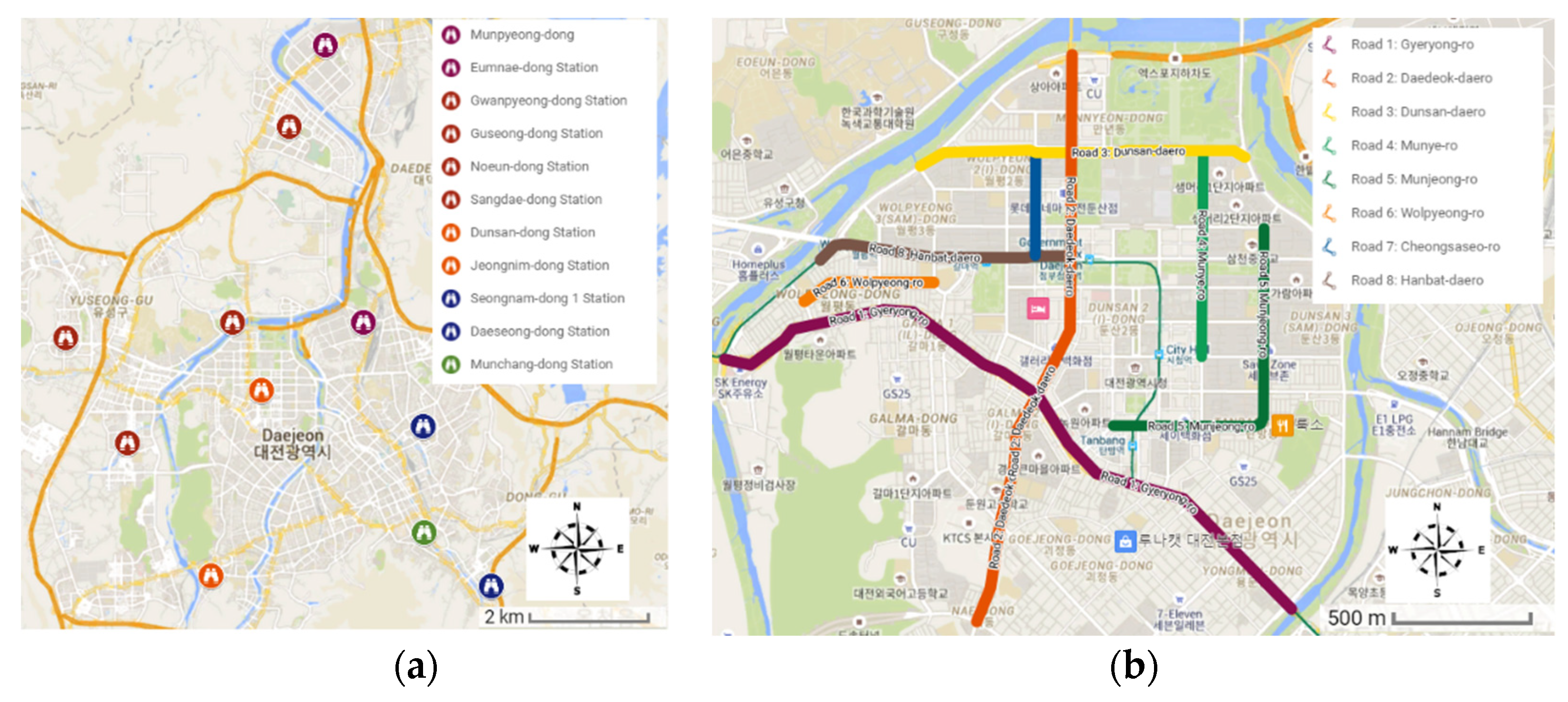
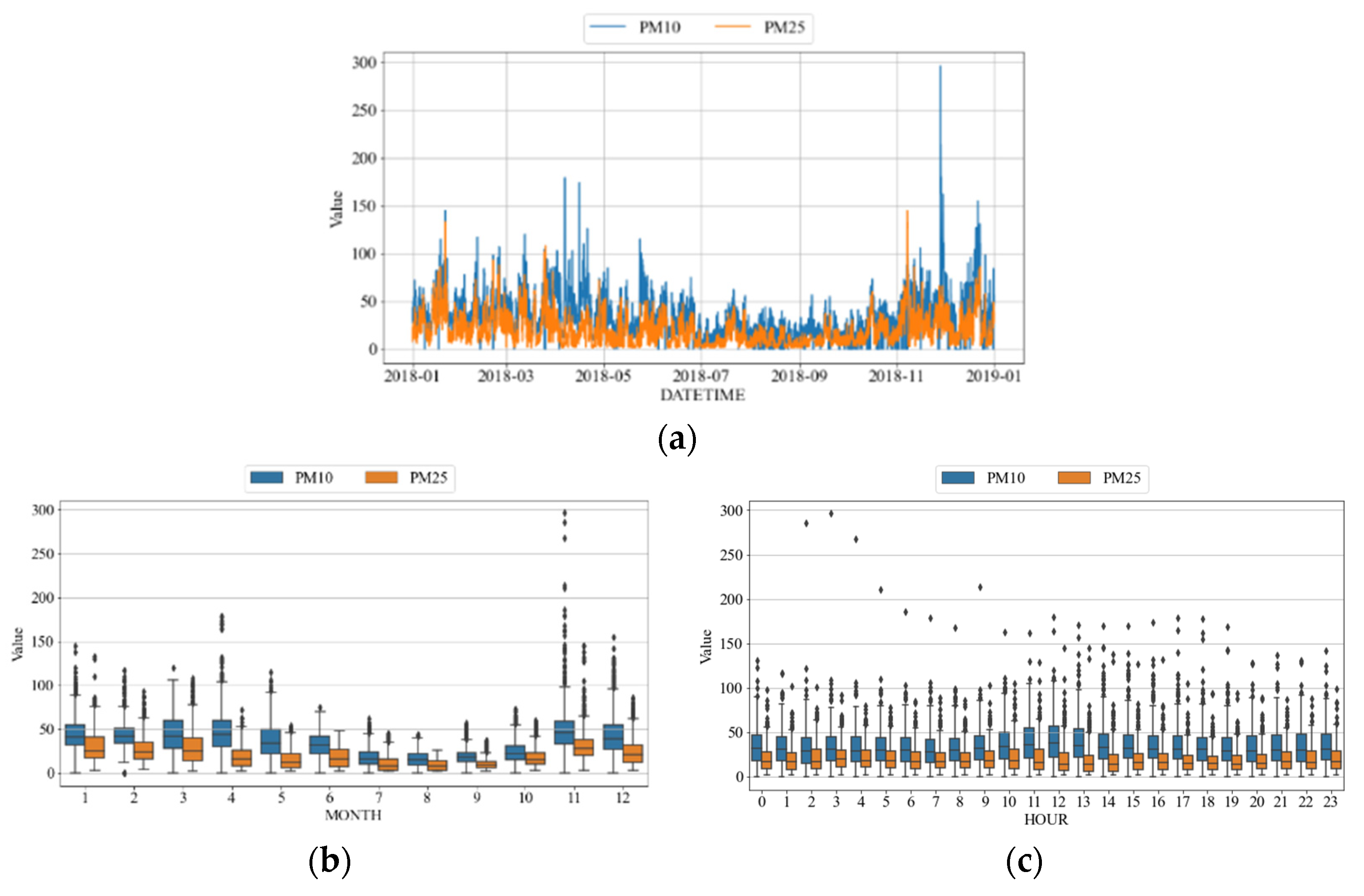
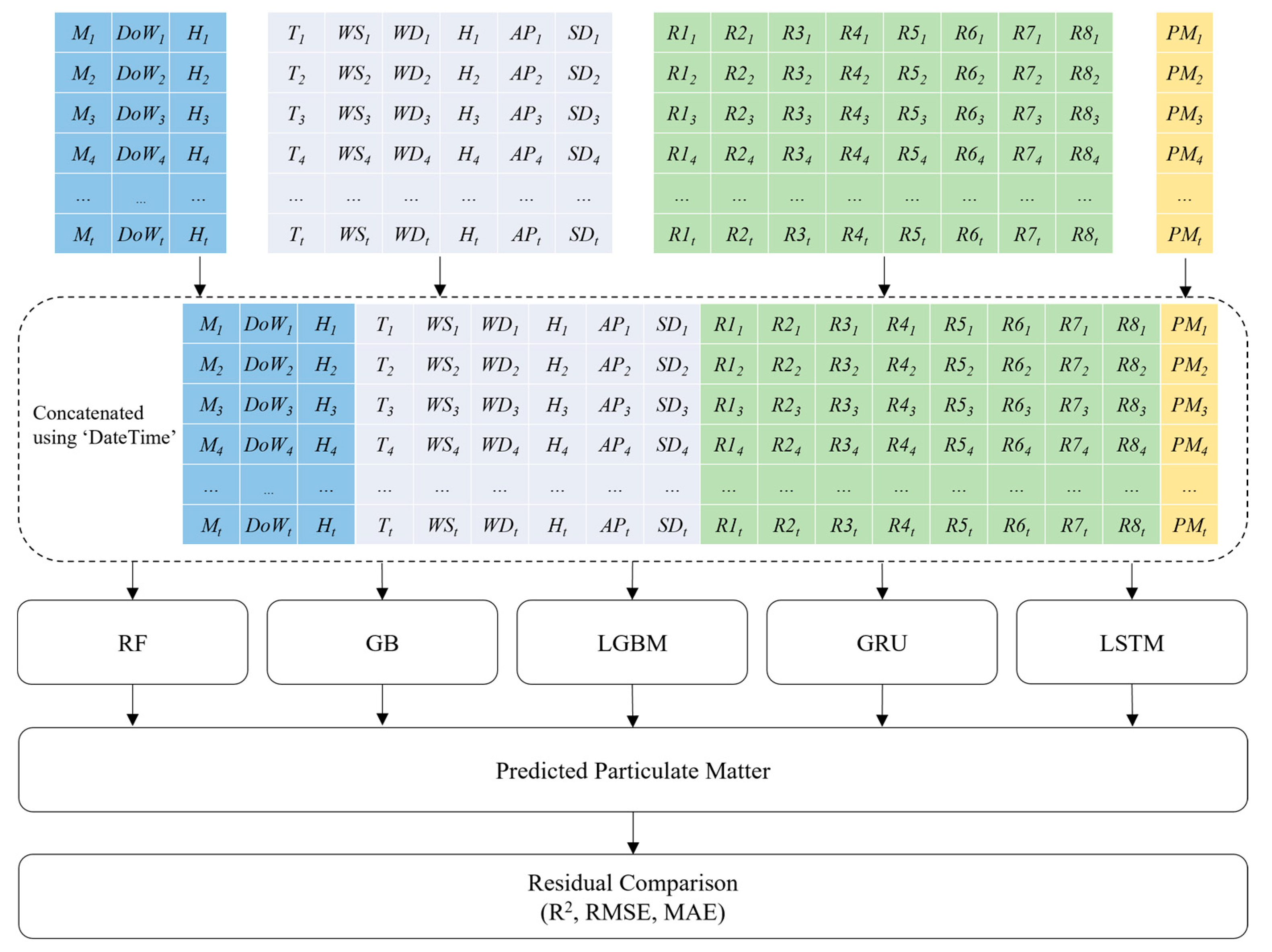
- First, we collected meteorological data from 11 air pollution measurement stations and traffic data from eight roads in Daejeon from 1 January 2018 to 31 December 2018. Then, we preprocessed the datasets to obtain a final dataset for our prediction models. The preprocessing consisted of the following steps: (1) consolidating the datasets, (2) cleaning invalid data, and (3) filling in missing data.
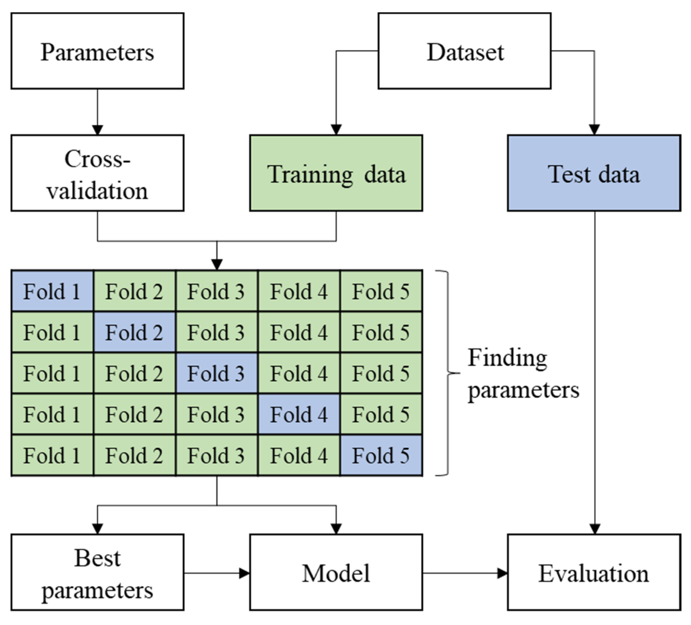
- Furthermore, we evaluated the performance of several machine learning and deep learning models for predicting the PM concentration. We selected the RF, gradient boosting (GB), and light gradient boosting (LGBM) machine learning models. In addition, we selected the gated recurrent unit (GRU) and long short-term memory (LSTM) deep learning models. We determined the optimal accuracy of each model by selecting the best parameters using a cross-validation technique. Experimental evaluations showed that the deep learning models outperformed the machine learning models in predicting PM concentrations in Daejeon.
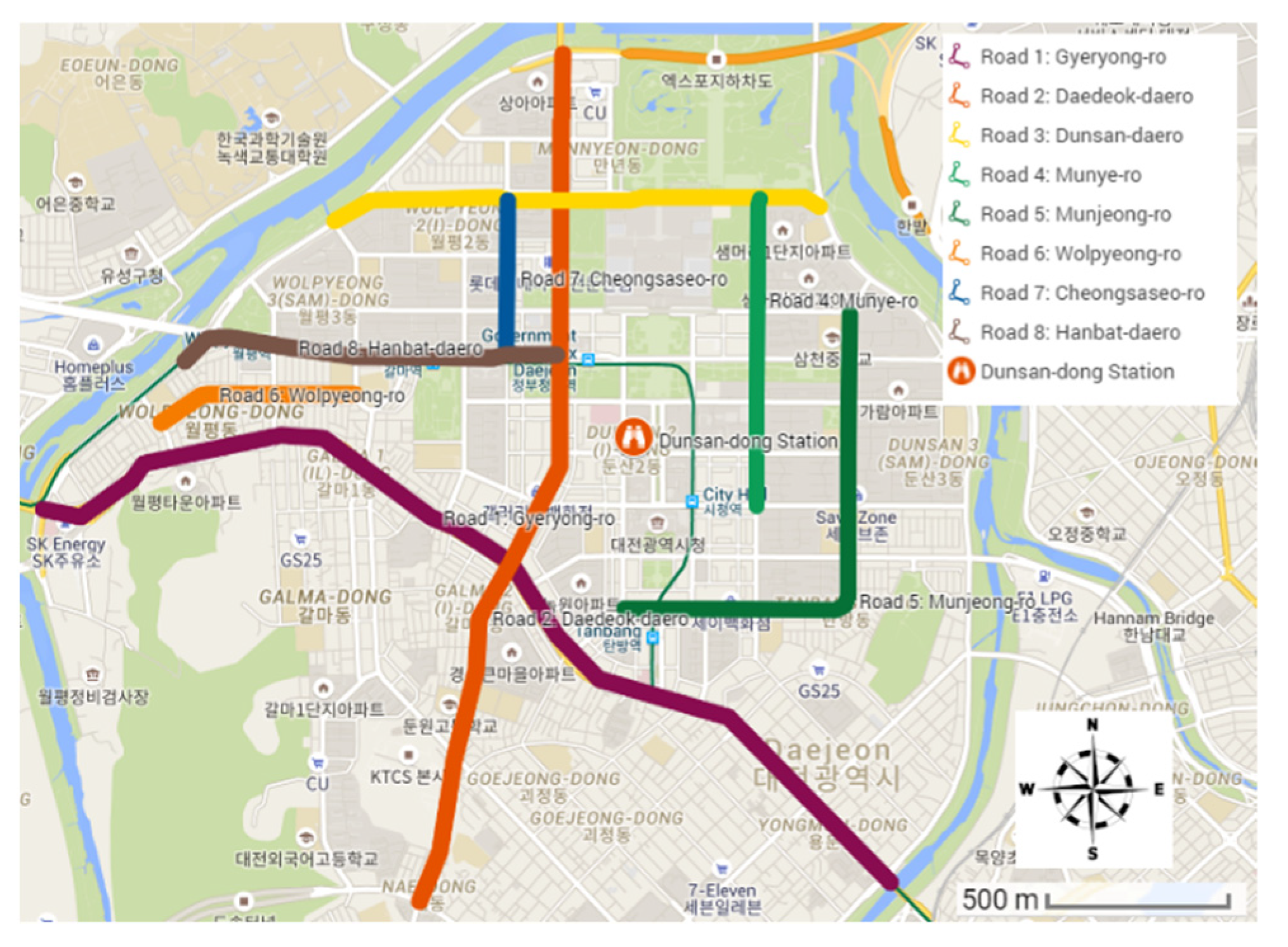
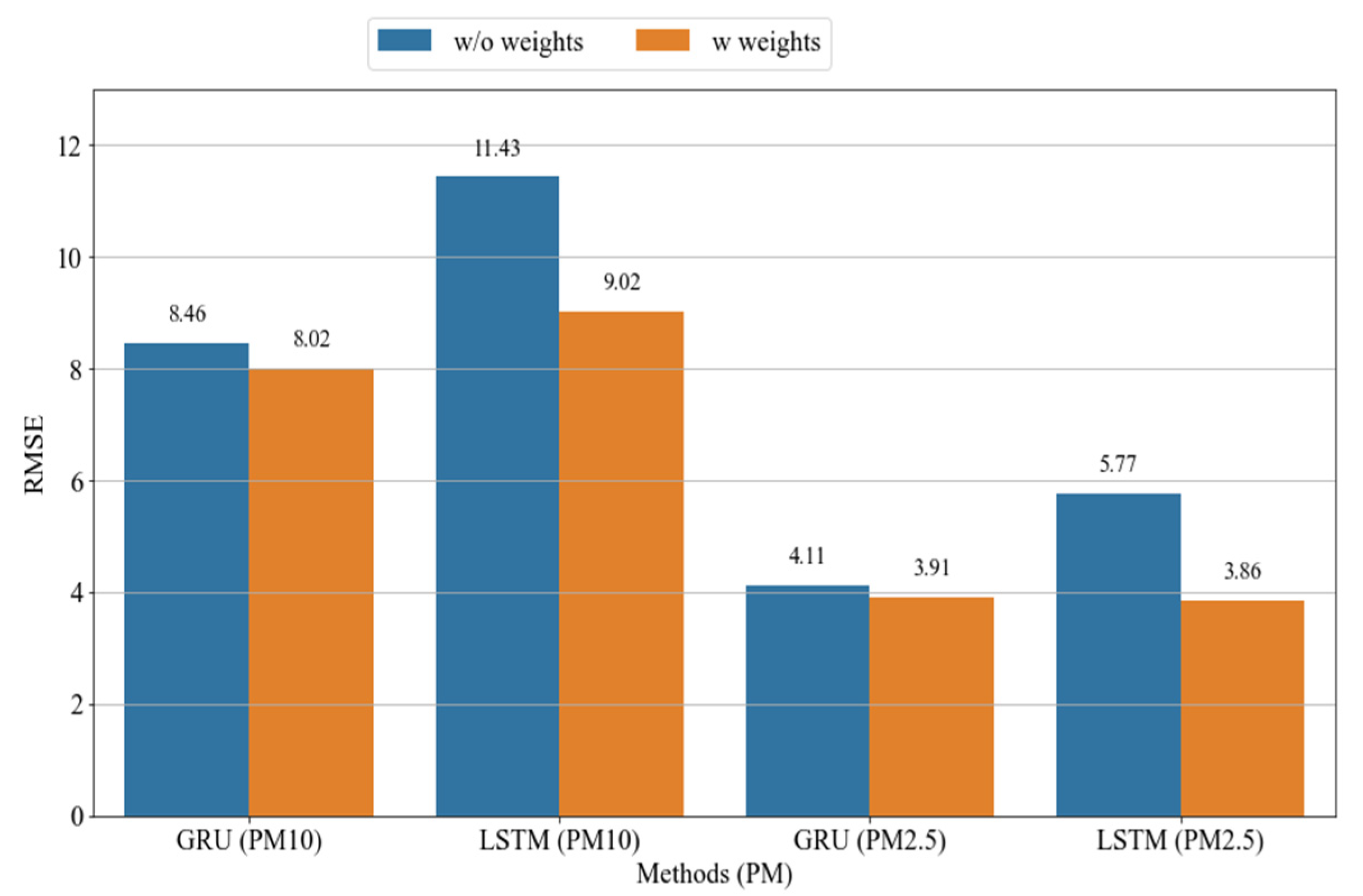
- Finally, we measured the influence of the road conditions on the prediction of PM concentrations. Specifically, we developed a method that set road weights on the basis of the stations, road locations, wind direction, and wind speed. An air pollution measurement station surrounded by eight roads was selected for this purpose. Experimental results demonstrated that the proposed method of using road weights decreased the error rates of the predictive models by up to 21% and 33% for PM10 and PM2.5, respectively.
2. Related Work
2.1. Prediction of AQI Using Meteorological Data
2.2. Prediction of AQI Using Traffic Data
2.3. Prediction of AQI Using Meteorological and Traffic Data
3. Materials and Methods
3.1. Overview
3.2. Study Area
3.3. Data Collection
3.4. Competing Models
- : Time steps.
- : Candidate cell and final cell state at time step . The candidate cell state is also referred to as the hidden state.
- : Weight matrices.
- : Bias vectors.
- : Update gate, reset gate, insert gate, forget gate, and output gate, respectively.
- : Activation functions.
3.5. Evaluation Metrics
4. Results
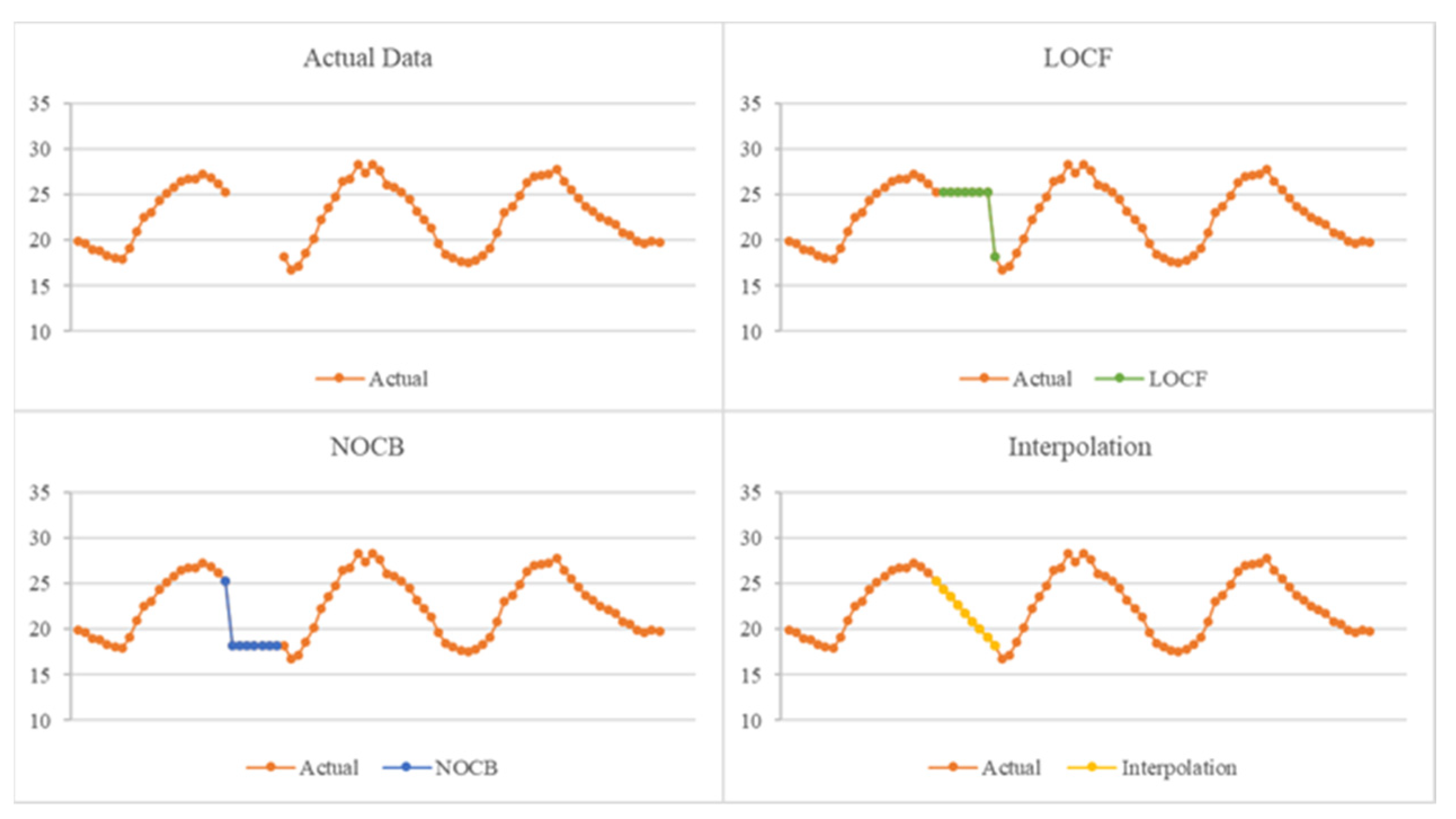
4.1. Preprocessing
- Last observation carried forward (LOCF): The last observed non-missing value was used to fill the missing values at later points.
- Next observation carried backward (NOCB): The next non-missing observation was used to fill the missing values at earlier points.
- Interpolation: New data points were constructed within the range of a discrete set of known data.
4.2. Training of Models
4.3. Experimental Results
4.3.1. Hyperparameters of Competing Models
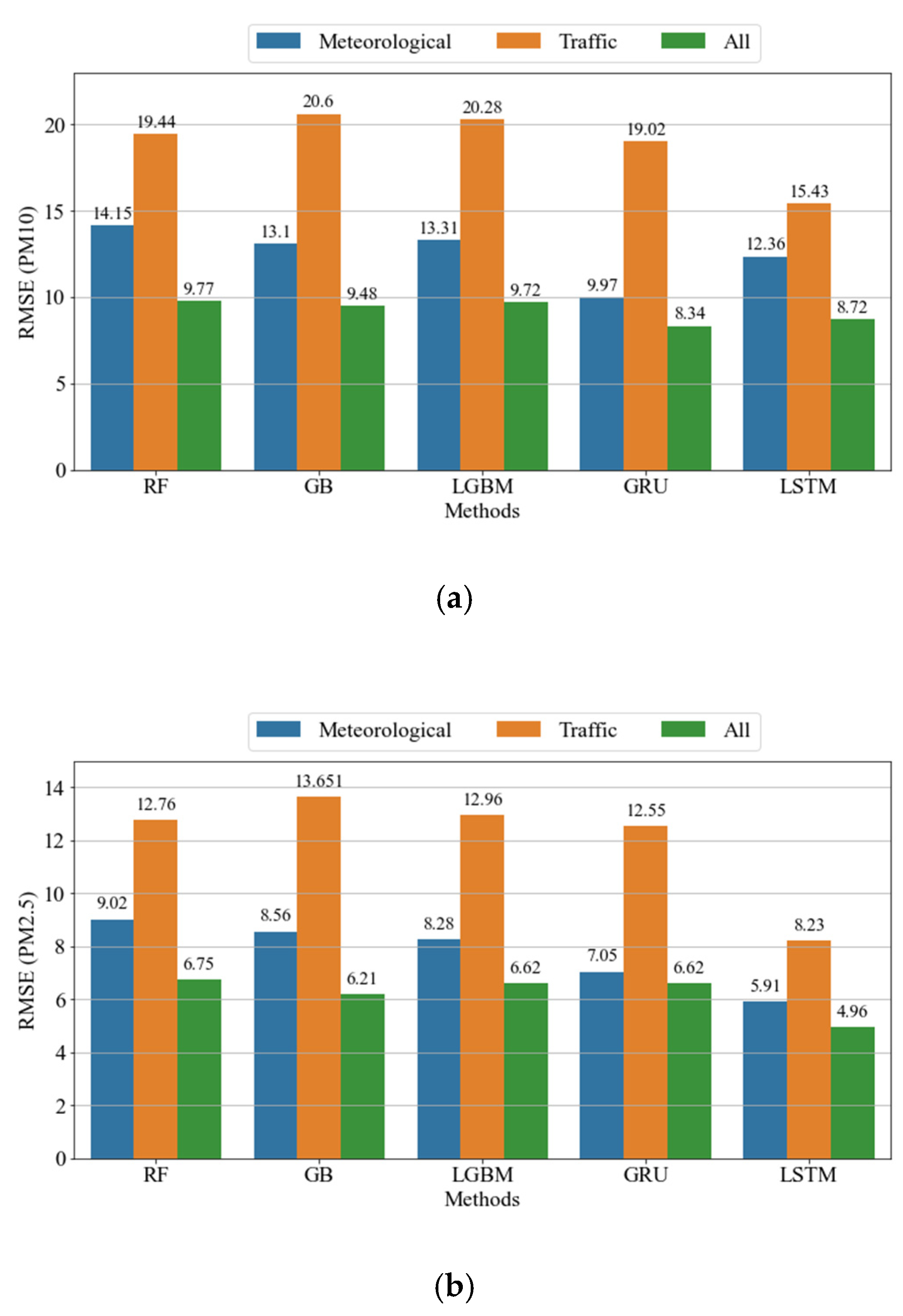
4.3.2. Impacts of Different Features
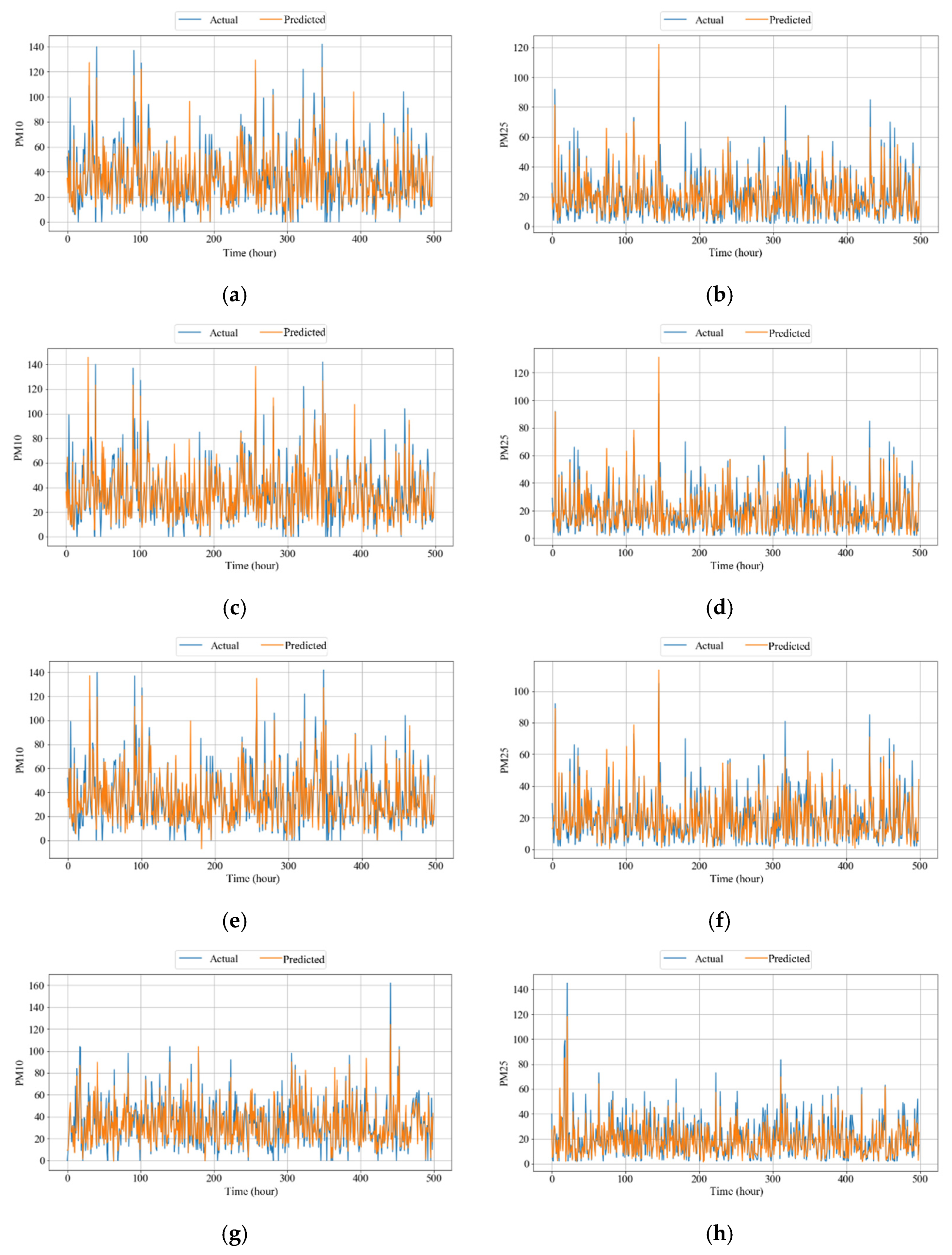
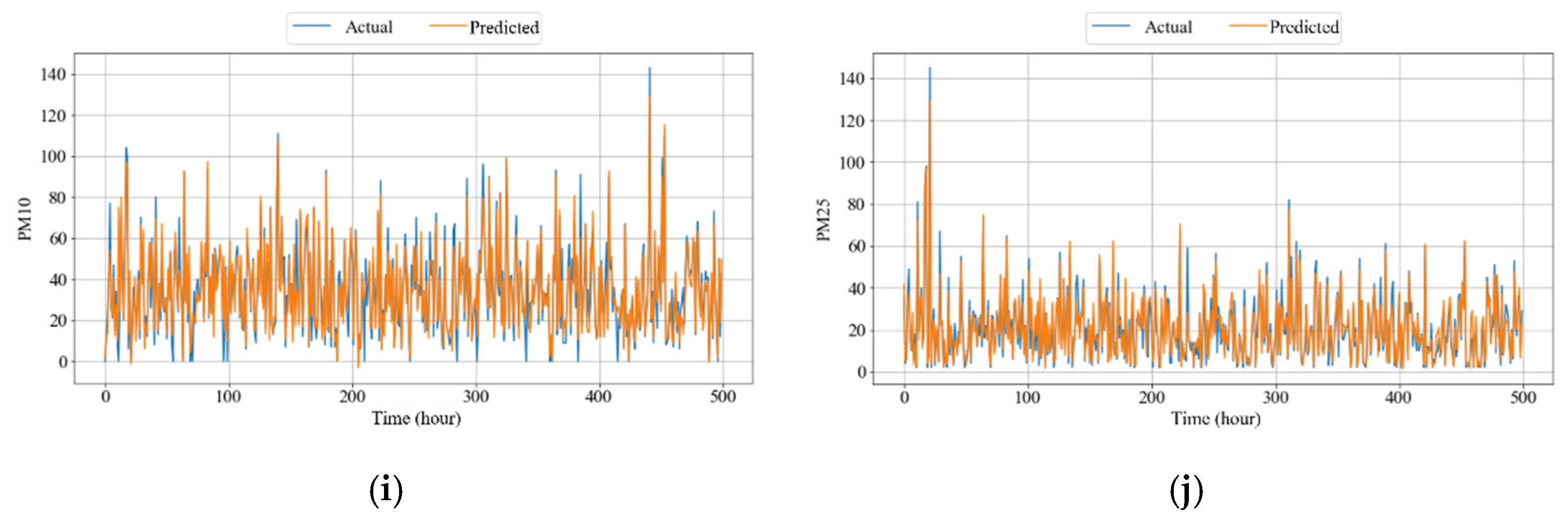
4.3.3. Comparison of Competing Models
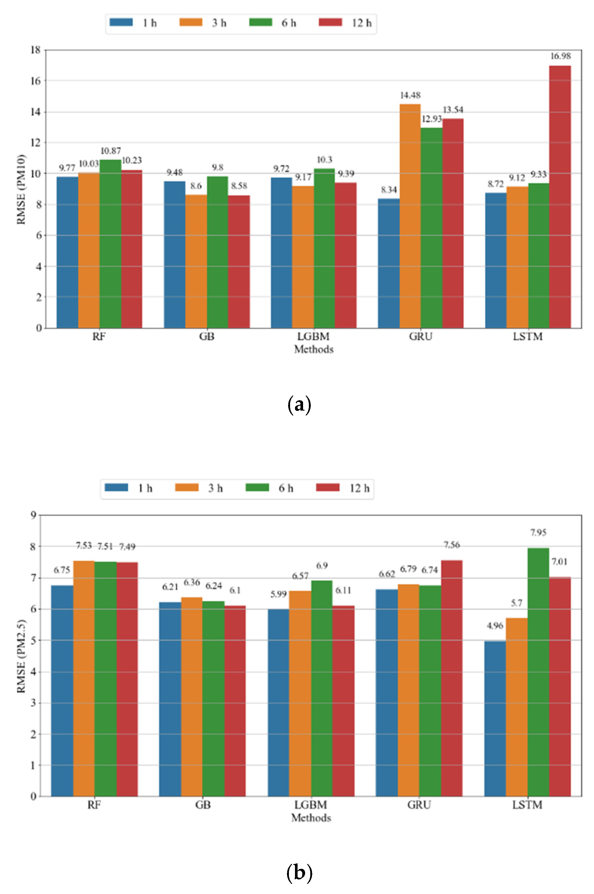
4.3.4. Comparison of Prediction Time
4.3.5. Influence of Wind Direction and Speed
5. Discussion and Conclusions
Author Contributions
Funding
Institutional Review Board Statement
Informed Consent Statement
Data Availability Statement
Conflicts of Interest
References
- Almetwally, A.A.; Bin-Jumah, M.; Allam, A.A. Ambient air pollution and its influence on human health and welfare: An overview. Environ. Sci. Pollut. Res. 2020, 27, 24815–24830. [Google Scholar] [CrossRef]
- Manisalidis, I.; Stavropoulou, E.; Stavropoulos, A.; Bezirtzoglou, E. Environmental and health impacts of air pollution: A review. Front. Public Health 2020, 8, 14. [Google Scholar] [CrossRef] [PubMed] [Green Version]
- Koo, J.H.; Kim, J.; Lee, Y.G.; Park, S.S.; Lee, S.; Chong, H.; Cho, Y.; Kim, J.; Choi, K.; Lee, T. The implication of the air quality pattern in South Korea after the COVID-19 outbreak. Sci. Rep. 2020, 10, 22462. [Google Scholar] [CrossRef]
- World Health Organization. Available online: https://www.who.int/mediacentre/news/releases/2014/air-pollution/en (accessed on 10 February 2021).
- Zhao, C.X.; Wang, Y.Q.; Wang, Y.J.; Zhang, H.L.; Zhao, B.Q. Temporal and spatial distribution of PM2.5 and PM10 pollution status and the correlation of particulate matters and meteorological factors during winter and spring in Beijing. Environ. Sci. 2014, 35, 418–427. [Google Scholar]
- Annual Report of Air Quality in Korea 2018; National Institute of Environmental Research: Incheon, Korea, 2019.
- Shapiro, M.A.; Bolsen, T. Transboundary air pollution in South Korea: An analysis of media frames and public attitudes and behavior. East Asian Community Rev. 2018, 1, 107–126. [Google Scholar] [CrossRef]
- Kim, H.C.; Kim, S.; Kim, B.U.; Jin, C.S.; Hong, S.; Park, R.; Son, S.W.; Bae, C.; Bae, M.A.; Song, C.K.; et al. Recent increase of surface particulate matter concentrations in the Seoul Metropolitan Area, Korea. Sci. Rep. 2017, 7, 4710. [Google Scholar] [CrossRef] [PubMed] [Green Version]
- Korean Statistical Information Service. Available online: https://kosis.kr/eng/statisticsList/statisticsListIndex.do?menuId=M_01_01 (accessed on 10 February 2021).
- Hitchcock, G.; Conlan, B.; Branningan, C.; Kay, D.; Newman, D. Air Quality and Road Transport—Impacts and Solutions; RAC Foundation: London, UK, 2014. [Google Scholar]
- Daejeon Metropolitan City. Available online: https://www.daejeon.go.kr/dre/index.do (accessed on 2 March 2021).
- Kim, H.; Kim, H.; Lee, J.T. Effect of air pollutant emission reduction policies on hospital visits for asthma in Seoul, Korea; Quasi-experimental study. Environ. Int. 2019, 132, 104954. [Google Scholar] [CrossRef] [PubMed]
- Lee, S.; Kim, S.; Kim, H.; Seo, Y.; Ha, Y.; Kim, H.; Ha, R.; Yu, Y. Tracing of traffic-related pollution using magnetic properties of topsoils in Daejeon, Korea. Environ. Earth Sci. 2020, 79, 485. [Google Scholar] [CrossRef]
- Dasari, K.B.; Cho, H.; Jaćimović, R.; Sun, G.M.; Yim, Y.H. Chemical composition of Asian dust in Daejeon, Korea, during the spring season. ACS Earth Space Chem. 2020, 4, 1227–1236. [Google Scholar] [CrossRef]
- Jeong, Y.; Youn, Y.; Cho, S.; Kim, S.; Huh, M.; Lee, Y. Prediction of Daily PM10 Concentration for Air Korea Stations Using Artificial Intelligence with LDAPS Weather Data, MODIS AOD, and Chinese Air Quality Data. Korean J. Remote Sens. 2020, 36, 573–586. [Google Scholar]
- Park, J.; Chang, S. A particulate matter concentration prediction model based on long short-term memory and an artificial neural network. Int. J. Environ. Res. Public Health 2021, 18, 6801. [Google Scholar] [CrossRef]
- Kim, S.-Y.; Song, I. National-scale exposure prediction for long-term concentrations of particulate matter and nitrogen dioxide in South Korea. Environ. Pollut. 2017, 226, 21–29. [Google Scholar] [CrossRef]
- Eum, Y.; Song, I.; Kim, H.-C.; Leem, J.-H.; Kim, S.-Y. Computation of geographic variables for air pollution prediction models in South Korea. Environ. Health Toxicol. 2015, 30, e2015010. [Google Scholar] [CrossRef] [Green Version]
- Jang, E.; Do, W.; Park, G.; Kim, M.; Yoo, E. Spatial and temporal variation of urban air pollutants and their concentrations in relation to meteorological conditions at four sites in Busan, South Korea. Atmos. Pollut. Res. 2017, 8, 89–100. [Google Scholar] [CrossRef]
- Lee, M.; Lin, L.; Chen, C.Y.; Tsao, Y.; Yao, T.H.; Fei, M.H.; Fang, S.H. Forecasting air quality in Taiwan by using machine learning. Sci. Rep. 2020, 10, 4153. [Google Scholar] [CrossRef]
- Chang, Z.; Guojun, S. Application of data mining to the analysis of meteorological data for air quality prediction: A case study in Shenyang. IOP Conf. Ser. Earth Environ. Sci. 2017, 81, 012097. [Google Scholar]
- Choubin, B.; Abdolshahnejad, M.; Moradi, E.; Querol, X.; Mosavi, A.; Shamshirband, S.; Ghamisi, P. Spatial hazard assessment of the PM10 using machine learning models in Barcelona, Spain. Sci. Total Environ. 2020, 701, 134474. [Google Scholar] [CrossRef]
- Qadeer, K.; Rehman, W.U.; Sheri, A.M.; Park, I.; Kim, H.K.; Jeon, M. A long short-term memory (LSTM) network for hourly estimation of PM2.5 concentration in two cities of South Korea. Appl. Sci. 2020, 10, 3984. [Google Scholar] [CrossRef]
- Xayasouk, T.; Lee, H.; Lee, G. Air pollution prediction using long short-term memory (LSTM) and deep autoencoder (DAE) models. Sustainability 2020, 12, 2570. [Google Scholar] [CrossRef] [Green Version]
- Comert, G.; Darko, S.; Huynh, N.; Elijah, B.; Eloise, Q. Evaluating the impact of traffic volume on air quality in South Carolina. Int. J. Transp. Sci. Technol. 2020, 9, 29–41. [Google Scholar] [CrossRef]
- Adams, M.D.; Requia, W.J. How private vehicle use increases ambient air pollution concentrations at schools during the morning drop-off of children. Atmos. Environ. 2017, 165, 264–273. [Google Scholar] [CrossRef]
- Askariyeh, M.H.; Venugopal, M.; Khreis, H.; Birt, A.; Zietsman, J. Near-road traffic-related air pollution: Resuspended PM2.5 from highways and arterials. Int. J. Environ. Res. Public Health 2020, 17, 2851. [Google Scholar] [CrossRef]
- Rossi, R.; Ceccato, R.; Gastaldi, M. Effect of road traffic on air pollution. Experimental evidence from COVID-19 lockdown. Sustainability 2020, 12, 8984. [Google Scholar] [CrossRef]
- Lešnik, U.; Mongus, D.; Jesenko, D. Predictive analytics of PM10 concentration levels using detailed traffic data. Transp. Res. D Transp. Environ. 2019, 67, 131–141. [Google Scholar] [CrossRef]
- Wei, Z.; Peng, J.; Ma, X.; Qiu, S.; Wangm, S. Toward periodicity correlation of roadside PM2.5 concentration and traffic volume: A wavelet perspective. IEEE Trans. Veh. Technol. 2019, 68, 10439–10452. [Google Scholar] [CrossRef]
- Catalano, M.; Galatioto, F.; Bell, M.; Namdeo, A.; Bergantino, A.S. Improving the prediction of air pollution peak episodes generated by urban transport networks. Environ. Sci. Policy 2016, 60, 69–83. [Google Scholar] [CrossRef] [Green Version]
- Askariyeh, M.H.; Zietsman, J.; Autenrieth, R. Traffic contribution to PM2.5 increment in the near-road environment. Atmos. Environ. 2020, 224, 117113. [Google Scholar] [CrossRef]
- Korea Environment Corporation. Available online: https://www.airkorea.or.kr/ (accessed on 2 March 2021).
- Korea Meteorological Administration. Available online: https://www.kma.go.kr/eng/index.jsp (accessed on 2 March 2021).
- Daejeon Transportation Data Warehouse. Available online: http://tportal.daejeon.go.kr/ (accessed on 2 March 2021).
- Breiman, L. Random forests. Mach. Learn. 2001, 45, 5–32. [Google Scholar] [CrossRef] [Green Version]
- Friedman, J.H. Greedy function approximation: A gradient boosting machine. Ann. Statist. 2001, 29, 1189–1232. [Google Scholar] [CrossRef]
- Ke, G.; Meng, Q.; Finley, T.; Wang, T.; Chen, W.; Ma, W.; Ye, Q.; Liu, T.-Y. LightGBM: A highly efficient gradient boosting decision tree. Adv. Neural Inf. Process. Syst. 2017, 30, 3149–3157. [Google Scholar]
- Chung, J.; Gulcehre, C.; Cho, K.H.; Bengio, Y. Empirical evaluation of gated recurrent neural networks on sequence modeling. arXiv 2014, arXiv:1412.3555. [Google Scholar]
- Hochreiter, S.; Schmidhuber, J. Long short-term memory. Neural Comput. 1997, 9, 1735–1780. [Google Scholar] [CrossRef]
- Pedregosa, F.; Varoquaux, G.; Gramfort, A.; Michel, V.; Thirion, B.; Grisel, O.; Blondel, M.; Prettenhofer, P.; Weiss, R.; Dubourg, V.; et al. Scikit-learn: Machine learning in Python. J. Mach. Learn. Res. 2011, 12, 2825–2830. [Google Scholar]
- Kim, K.H.; Lee, S.B.; Woo, D.; Bae, G.N. Influence of wind direction and speed on the transport of particle-bound PAHs in a roadway environment. Atmos. Pollut. Res. 2015, 6, 1024–1034. [Google Scholar] [CrossRef]
- Kim, Y.; Guldmann, J.M. Impact of traffic flows and wind directions on air pollution concentrations in Seoul, Korea. Atmos. Environ. 2011, 45, 2803–2810. [Google Scholar] [CrossRef]
- Guerra, S.A.; Lane, D.D.; Marotz, G.A.; Carter, R.E.; Hohl, C.M.; Baldauf, R.W. Effects of wind direction on coarse and fine particulate matter concentrations in southeast Kansas. J. Air Waste Manag. Assoc. 2006, 56, 1525–1531. [Google Scholar] [CrossRef] [Green Version]


| Variable Name | Count | Mean | Min | Max | Std | Missing Value |
|---|---|---|---|---|---|---|
| PM2.5 | 8342 | 20.185447 | 2 | 145 | 15.808386 | 418 |
| PM10 | 8760 | 35.118607 | 0 | 296 | 23.372221 | 0 |
| TEMPERATURE | 8756 | 13.593 | −16 | 39.3 | 11.593 | 4 |
| WIND_SPEED | 8760 | 1.552 | 0 | 8.3 | 1.16 | 0 |
| WIND_DIRECTION | 8760 | 201.705 | 0 | 360 | 124.023 | 0 |
| HUMIDITY | 8746 | 68.954 | 14 | 98 | 19.777 | 14 |
| AIR_PRESSURE | 8760 | 1008.918 | 979.6 | 1030.7 | 8.129 | 0 |
| SNOW_DEPTH | 270 | 3.088 | 0 | 7.9 | 2.015 | 8490 |
| ROAD_1 | 8328 | 38.275 | 0 | 58.489 | 9.614 | 432 (N/A) + 501 (Zero) |
| ROAD_2 | 8328 | 52.994 | 0 | 75.691 | 10.1 | 432 (N/A) + 501 (Zero) |
| ROAD_3 | 8328 | 39.371 | 0 | 62.828 | 11.078 | 432 (N/A) + 501 (Zero) |
| ROAD_4 | 8328 | 43.682 | 0 | 64.895 | 10.66 | 432 (N/A) + 501 (Zero) |
| ROAD_5 | 8328 | 41.353 | 0 | 68.33 | 12.375 | 432 (N/A) + 501 (Zero) |
| ROAD_6 | 8328 | 41.063 | 0 | 53.382 | 6.332 | 432 (N/A) + 501 (Zero) |
| ROAD_7 | 8328 | 36.027 | 0 | 61.022 | 11.231 | 432 (N/A) + 501 (Zero) |
| ROAD_8 | 8328 | 42.825 | 0 | 65.912 | 11.786 | 432 (N/A) + 501 (Zero) |
| Model | Parameter | Description | Options | Selected |
|---|---|---|---|---|
| RF | n_estimators | Number of trees in the forest | 100, 200, 300, 500, 1000 | 500 |
| max_features | Maximum number of features on each split | auto, sqrt, log2 | auto | |
| max_depth | Maximum depth in each tree | 70, 80, 90, 100 | 80 | |
| min_samples_split | Minimum number of samples of parent node | 3, 4, 5 | 3 | |
| min_samples_leaf | Minimum number of samples to be at a leaf node | 8, 10, 12 | 8 | |
| GB | n_estimators | Number of trees in the forest | 100, 200, 300, 500, 1000 | 100 |
| max_features | Maximum number of features on each split | auto, sqrt, log2 | auto | |
| max_depth | Maximum depth in each tree | 80, 90, 100, 110 | 90 | |
| min_samples_split | Minimum number of samples of parent node | 2, 3, 5 | 2 | |
| min_samples_leaf | Minimum number of samples of parent node | 1, 8, 9, 10 | 8 | |
| LGBM | n_estimators | Number of trees in the forest | 100, 200, 300, 500, 1000 | 1000 |
| max_depth | Maximum depth in each tree | 80, 90, 100, 110 | 80 | |
| num_leaves | Maximum number of leaves | 8, 12, 16, 20 | 20 | |
| min_split_gain | Minimum number of samples of parent node | 2, 3, 5 | 2 | |
| min_child_samples | Minimum number of samples of parent node | 1, 8, 9, 10 | 9 | |
| GRU | seq_length | Number of values in a sequence | 18, 20, 24 | 24 |
| batch_size | Number of samples in each batch during training and testing | 64 | 64 | |
| epochs | Number of times that entire dataset is learned | 200 | 200 | |
| patience | Number of epochs for which the model did not improve | 10 | 10 | |
| learning_rate | Tuning parameter of optimization | 0.01, 0.1 | 0.01 | |
| layers | GRU block of deep learning model | 3, 5, 7 | 3 | |
| units | Neurons of GRU model | 50, 100, 120 | 50 | |
| LSTM | seq_length | Number of values in a sequence | 18, 20, 24 | 24 |
| batch_size | Number of samples in each batch during training and testing | 64 | 64 | |
| epochs | Number of times that entire dataset is learned | 200 | 200 | |
| patience | Number of epochs for which the model did not improve | 10 | 10 | |
| learning_rate | Tuning parameter of optimization | 0.01, 0.1 | 0.01 | |
| layers | LSTM block of deep learning model | 3, 5, 7 | 5 | |
| units | Neurons of LSTM model | 64, 128, 256 | 128 |
| Model | PM10 | PM2.5 | ||||
|---|---|---|---|---|---|---|
| R2 | RMSE | MAE | R2 | RMSE | MAE | |
| RF | 83.71% | 9.77 | 6.73 | 82.16% | 6.75 | 4.79 |
| GB | 84.66% | 9.48 | 6.4 | 84.88% | 6.21 | 4.27 |
| LGBM | 83.87% | 9.72 | 6.72 | 85.93% | 5.99 | 4.35 |
| GRU | 85.62% | 8.34 | 5.07 | 84.01% | 6.62 | 4.84 |
| LSTM | 84.81% | 8.72 | 5.41 | 91.16% | 4.96 | 3.44 |
| Id | Numerical Value | Categorical Value | Roads |
|---|---|---|---|
| 1 | 1°–90° | NE | 3, 4, 5 |
| 2 | 91°–180° | SE | 1, 4, 5 |
| 3 | 181°–270° | SW | 1, 2, 5, 6 |
| 4 | 271°–360° | NW | 1, 2, 6, 7, 8 |
Publisher’s Note: MDPI stays neutral with regard to jurisdictional claims in published maps and institutional affiliations. |
© 2021 by the authors. Licensee MDPI, Basel, Switzerland. This article is an open access article distributed under the terms and conditions of the Creative Commons Attribution (CC BY) license (https://creativecommons.org/licenses/by/4.0/).
Share and Cite
Chuluunsaikhan, T.; Heak, M.; Nasridinov, A.; Choi, S. Comparative Analysis of Predictive Models for Fine Particulate Matter in Daejeon, South Korea. Atmosphere 2021, 12, 1295. https://doi.org/10.3390/atmos12101295
Chuluunsaikhan T, Heak M, Nasridinov A, Choi S. Comparative Analysis of Predictive Models for Fine Particulate Matter in Daejeon, South Korea. Atmosphere. 2021; 12(10):1295. https://doi.org/10.3390/atmos12101295
Chicago/Turabian StyleChuluunsaikhan, Tserenpurev, Menghok Heak, Aziz Nasridinov, and Sanghyun Choi. 2021. "Comparative Analysis of Predictive Models for Fine Particulate Matter in Daejeon, South Korea" Atmosphere 12, no. 10: 1295. https://doi.org/10.3390/atmos12101295
APA StyleChuluunsaikhan, T., Heak, M., Nasridinov, A., & Choi, S. (2021). Comparative Analysis of Predictive Models for Fine Particulate Matter in Daejeon, South Korea. Atmosphere, 12(10), 1295. https://doi.org/10.3390/atmos12101295