1. Introduction
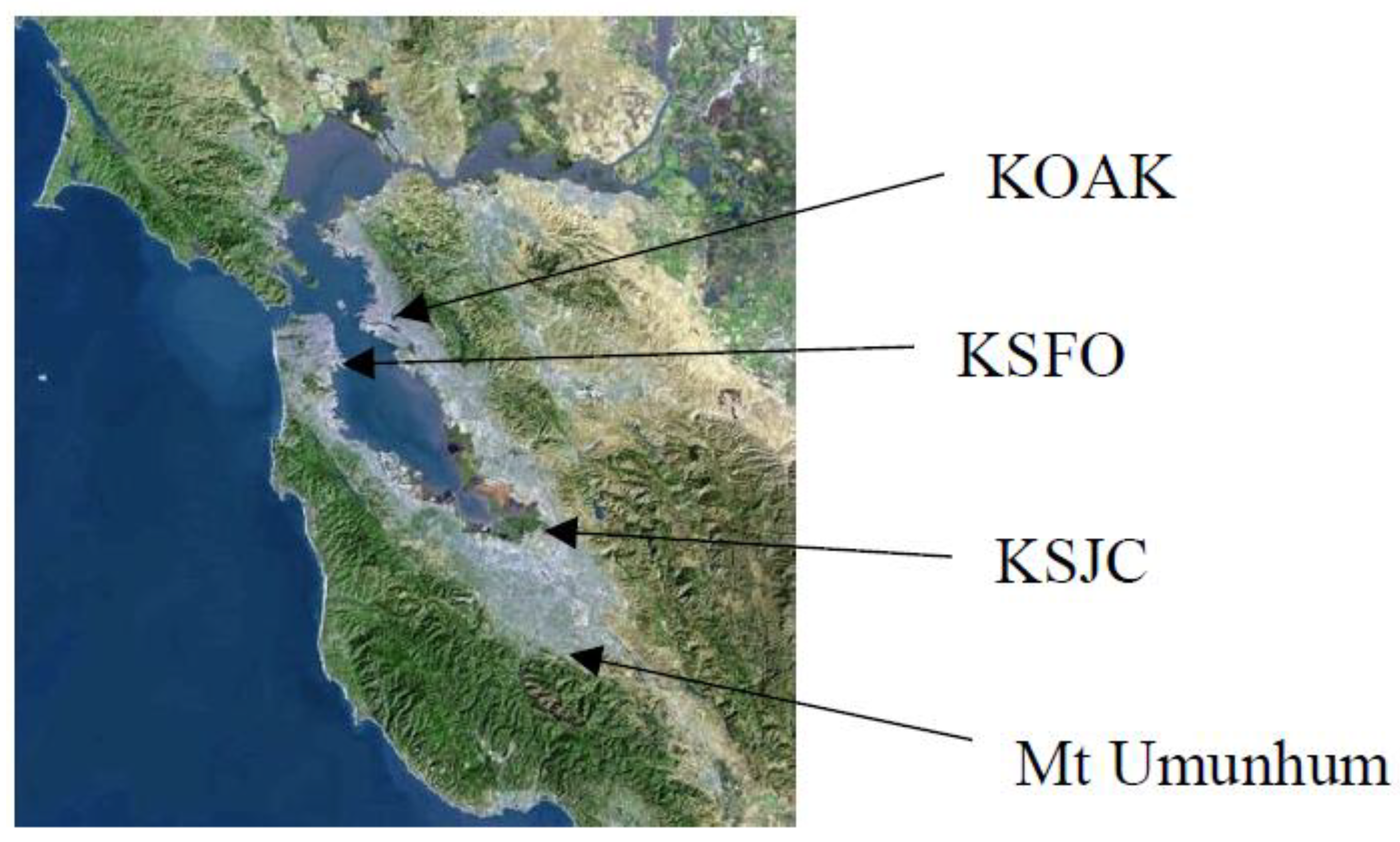
There is an obvious need for accurate rainfall forecasting on the local scale, especially in high population areas. During heavy rain events, accurate forecasts with a 24–48 h lead time can allow emergency managers to prepare for flash flooding and other high-water situations. Water managers can also make decisions in order to prepare for rapid input into reservoirs. One such situation occurred in San Jose, CA as a result of the 20 February 2017 rain event (local geography of the study region is shown in
Figure 1). After several rainy days, one particularly wet day–an atmospheric river (AR) event–combined with a release of water from an area dam, resulted in unexpected flooding along a local river in San Jose (SJ). Multiple water rescues had to be performed, and many houses were flooded (see the discussion below in
Section 4.1). On a more mundane level, the city of SJ receives roughly half its drinking water from local groundwater resources, and these have to be replenished whenever possible–keeping in mind that most of California receives zero rain for roughly half the year. This is another challenge for local water managers (i.e., to replenish groundwater resources during the rainy season).
To better plan for rainfall–when and where and in what amounts it will fall–the community relies on state-of-the-art weather forecasting models. However, many local forecasters (e.g., on television) rely on models such as the Global Forecast System (GFS), whose resolution is too low to accurately capture rainfall variations in regions of complex terrain, such as the San Francisco Bay Area (SFBA). Especially in the Santa Clara valley (SCV), which is often in the rain shadow (RS) of the Santa Cruz (SC) mountains, this can result in dramatically wrong forecasts (e.g., multiple inches of rain forecast for a stormy week, whereas SJ could actually receive under an inch). In this study, the ability of the weather research and forecasting (WRF) model to accurately simulate local variations of rainfall in the SFBA during a variety of synoptic events was examined. Particular attention was focused on to the ability of WRF to capture the RS and the resulting rain in the SCV. We conducted three case studies of rain-producing synoptic weather events, each of which is presented as representative of “typical” SFBA events. One involves an AR impacting central California—these have the potential to produce large (by local standards) rainfall amounts, and may be expected to occur in central California 1–3 times each winter. The second involves a typical winter cold frontal passage. In non-drought years, there may be about 10–20 of these. The third is a similar event which produced rain everywhere except the SCV. No two rain-producing events are identical, and our study aimed at developing a configuration of WRF which can successfully predict characteristics of each of these storms, with the expectation that any successes will be replicated in similar synoptic events.
2. Background
A number of factors are involved in rain production, particularly in coastal California in the winter rain season. These include: the overall synoptic situation as it generates uplift (strength, structure, and proximity of synoptic features, and whether they are strengthening or decaying; whether or not an AR is present); local terrain and thermal influences (land-sea) on winds; the availability, location, and depth of moisture, as well as vertical temperature variation and stability; and cloud condensation nuclei (CCN) availability for condensation and deposition. These must all interact to produce rainfall. In addition, large spatial variation over regions such as the SFBA, which has both complex terrain and land-sea influences, leads to large spatial variations in rainfall accumulations.
Forecasts of rain (onset, duration, intensity) are made using numerical models, a number of which are available, and each of which has built-in trade-offs. The chief US models are the so-called GFS, NAM, and HRRR models. The global forecast system (GFS) model produces forecasts across a global domain out to 15 days or more, but at the expense of the spatial resolution needed to resolve rain variations on the mesoscale. At the moment, the resolution is 13 km for days 1–14, then 26 km beyond. The operational North American mesoscale forecast system (NAM) model runs out to 84 h with a resolution of 12 km. High-resolution (3 km) nested grid runs are also produced over some locations. Fine-scale models, such as the high-resolution rapid refresh (HRRR), improve upon the spatial resolution, but at the expense of the forecast horizon (e.g., the operational HRRR currently runs out to 18 h). The HRRR model has the ARW–WRF model at its core. The WRF model is in widespread use as an aid to forecasting at both NWS field offices and in various universities. All these models parameterize cloud and precipitation formation processes, and models such as WRF allow the user to choose from a number of schemes to do each of these processes. The ability of forecast models to predict rainfall totals and distributions accurately is continuing to improve, due to both observation and simulation campaigns to better understand cloud and precipitation microphysics processes, and also to improve abilities of numerical models to simulate all these elements. However, there is still room for improvement.
A number of prior studies using the WRF model have examined the range of solutions in various simulated fields (e.g., rainfall) when different model parameterizations are used. Some examples relevant to the west coast and ARs include: (i) a study of five AR events simulated using four choices of microphysics packages [
1]. Their comparison of observed and simulated total rainfall at point locations showed significant differences depending on which scheme was used, with all of them overestimating the total rain. Differences were also detected in liquid–ice partitioning within the simulated clouds. (ii) A simulation of one AR event and creation of “synthetic GOES (Geostationary Operational Environmental Satellite) imagery” [
2]. They ran WRF with five choices of microphysics packages, and compared various fields including 24 h rainfall (their Figure 7). Four of the five schemes produced very similar rainfall predictions. Synthetic brightness temperature fields revealed that the microphysics schemes were generating the total rainfall in different ways. (iii) A 20-year simulation of DJF rainfall patterns for 1980–2000 [
3], which produced good agreement with observations. In particular, they noted the ability of WRF to accurately capture the extreme precipitation and runoff events associated with ARs impacting the western states. (iv) A study of rain patterns in the SFBA during two AR events [
4]. Their simulations revealed rainfall rates that were higher during the event that involved significant bright band (BB) rainfall, as expected based on offshore observations that will be discussed below.
In coastal California, the majority of the winter rain (there is no summer rain) falls in association with synoptic events i.e., frontal passages, some with convection in the cold air behind. Some of these rain events are associated with ARs, which have been under intense study for several years now ([
5] and references therein). A typical AR is over 2000 km in length, but under 1000 km in width [
5]. The integrated vapor transport (IVT) in an AR ranges from 250 to over 1250 kg m
−1s
−1, and the duration ranges from under one to a few days [
5]. ARs account for 20–50% of annual rainfall (there is significant interannual variability), and almost all extreme rainfall events [
5]. As a result of the increased awareness and appreciation of the role and impacts of ARs, there have been campaigns (e.g., CALJET, [
6]) designed to reveal both broad and microphysical structures of ARs, using data from a variety of sources (satellites, dropsondes, satellite- and ground-based radar).
Two sets of AR studies are relevant to our work. First is a series of studies of the distribution and climatology of ARs. This has resulted in the development of a categorization of AR events [
5], and a catalog of AR events based on remotely-sensed water vapor distributions [
7,
8,
9]. The categories encompass impacts of ARs in the sense that those of long duration and/or high IVT can be hazardous via the flooding induced. The second set of studies is focused on the microphysics within an AR, and these can inform choices of parameterization schemes used in models, such as HRRR and WRF. One study used satellite retrievals to determine frequency distribution of warm vs cold vs mixed-phase rain regimes [
10]. They also determined mean rain rates associated with each regime. A significant number of events involved ice-phase precipitation, which is evidenced via a BB signal and resulting heavier rain rates. Analysis of landfalling ARs at coastal sites showed that non-BB rain events have smaller droplet sizes and lower rain rates when compared to BB rain events [
11]. GPM satellite radar measurements of precipitation parameters were analyzed for several offshore ARs [
12]. That study showed that GPM-measured BB elevations compared well to radar-based measurements taken along the coast, indicating that heaviest rain rates occurred in conjunction with the presence of a BB. These studies all suggest that high-end AR events will typically involve ice-phase precipitation formation, which must therefore be accounted for in models. COSMIC (Constellation Observing System for Meteorology, Ionosphere, and Climate) retrievals obtained during AR events have been examined, since they provide vertical profiles of temperature and moisture over the ocean just as land-based radiosondes would [
13]. The authors constructed composite soundings within an AR, as well as on the poleward and equatorward sides. These aid in the characterization of the thermodynamic structure of ARs, and can be compared with the AR case in this study.
Of the three rain events we examined, the heaviest rain was from an AR event, but two were non-AR. One involved a cold frontal passage with a short period of moderate rain, and post-frontal showers. This is the most typical synoptic rain event for the SFBA. Clearly some moisture is available in these cases, but the amount and areal extent do not rise to the level of an AR (i.e., atmospheric “puddles”). These events, although more common, are less hazardous, in that heavy rain and flooding events are almost always associated with ARs [
5]. There have been fewer in situ studies of the storm and frontal structures off the coast and over northern California.
Finally, we note that in the southern SFBA, the drinking water supply for business and consumers comes from local groundwater and, ultimately, from the Sierras in a roughly 50–50 balance. The area typically receives no rainfall from about May to mid-October. Winter rains in California are therefore critical in replenishing local groundwater, as well as in providing a snowpack in the Sierras. Accurate rain forecasts aid local water managers in their decision-making during both rain events and spring snowmelt events. Accurate forecasts of accumulated rainfall are obviously needed by emergency managers for various reasons, including planning for heavy rain events which can lead to flooding.
3. Synoptic Conditions
The SFBA typically experiences significant rain events from about mid-October to mid-May. On average there are about 36 rain events during this time frame that yield over 0.1” at San Jose Airport (SJC) in the SCV, and of these only 10 yield over 0.5” [
14] (location shown in
Figure 1). Some, but certainly not all of these rain events are linked to atmospheric river (AR) events [
5], although the majority of larger AR events are focused north of SF (e.g., Mendocino Coast).
A typical rain-producing synoptic event involves a surface low pressure system offshore north of the SFBA, with a trailing cold front (CF). It is the passage of these CFs that generates much of the rain over the SFBA. The rain that falls typically does so within a 6 h window. Rain rates may be quite heavy but only for about 1–2 h, resulting in relatively low overall accumulations. Given the latitude (e.g., SJC is at 37.3° N), fronts are typically weaker than those experienced further north. For the same reason, warm frontal passages, with more widespread and longer-lasting rains, are much more infrequent.
A feature of the SFBA is the complex terrain and shoreline (
Figure 1). A coastal range of hills runs NW–SE parallel to the coastline, and inland lies the SCV (also known as “Silicon Valley”). The highest peak to the east of SJC is Mt. Hamilton at ~1300 m, while to the south of SJC is Loma Prieta in the Santa Cruz mountains at ~1100 m. The hills due west of SJC are under ~700 m. These terrain barriers play an important role in determining the distribution of rain in the SFBA. At the same time, the spatial scale is quite small: as the crow flies, the distance between the two highest peaks is only ~30 km. The coastal range receives as much as 49” annually at Ben Lomond, with over 31” at Santa Cruz on the coast. Meanwhile, San Jose receives only 14.5” per year due to the rain shadow effect. To the east, Mt. Hamilton receives 23”. Hence, to accurately predict rainfall patterns, models must be capable of resolving quite small-scale terrain features, requiring high resolution in all three spatial dimensions. This is a densely populated and high-tech region, filled with people who notice when weather and rain forecasts are bad (and wonder why).
When thinking about planning for heavy rain events, water managers can look first to models such as the North American mesoscale forecast system (NAM) or GFS. The operational NAM runs out to 84 h with a resolution of 12 km, and nested NAM runs are also produced. The operational GFS has a resolution of 13 km when run out to 14 days, and then 26 km resolution for extended integrations. At these resolutions, neither the NAM nor the GFS can “see” local terrain well enough to accurately reproduce finer-scale details of the precipitation field in a region such as the SFBA. Instead, the NAM- and/or GFS-produced fields are used to initialize smaller-scale models, of which WRF is best known. Operationally, the HRRR model (with WRF at its core) runs hourly at a 3 km resolution, but produces forecasts only out to 18 h, not giving much advance time for planning. For water and local managers, a window of 24–48 h notice of heavy rain events allows more time for preparation. Thus, in this study, the ability of the WRF model “tuned” for the SFBA to simulate precipitation fields accurately was conducted. Details of the simulations are given in the next section.
4. Simulation Cases
We chose to examine the 2016–2017 rain year (1 July 2016–30 June 2017) since it had over 100% of normal rain in many parts of central California, including the SFBA. There were two significant rainy periods associated with ARs, and we chose the 20 February 2017 case since it also led to flooding. We were specifically interested in rain events in which the San Jose region received virtually zero rain compared to sites like SFO, a true RS. The 8 December 2016 case was chosen as representative of this group since the RS was so well-defined, with 0.01” rain over 24 h at SJC versus 1.32” at SFO (and 1.62” on the coast in Santa Cruz). There were about five such events in the rain year (identified largely by the rain amounts received elsewhere. For example, we deemed events with ~0.01” at SJC and ~0.2” at SFO as low-end rain events with no distinct separation in total rainfall between the two locations). Lastly, we looked for cases that were rain-producers but neither with an AR nor with a complete RS, as above. We characterize these as “typical” of rain-producers in the SFBA, where the rain falls in association with the passage of a cold front. More complete details are given below. We start with the wettest event, which was an AR event.
4.1. 20–21 February 2017
In February 2017, a series of AR events impacted California [
7], generating widespread heavy rains. The events of early February led to the near-collapse of the Oroville dam, which in turn led to evacuations on 12 February 2017. Rains returned a few days later in the form of more AR events. For the SFBA region, the 16 February 15Z surface analysis [
15] shows a cold front draped SW–NE across the SFBA, producing rain. Twenty-four hours later, a closed low was analyzed just offshore with a warm front producing more rain in the SFBA. Later, the associated cold front moved through and produced more rain. Thus, by 20 February, the ground in the SFBA was well soaked. The 00Z analysis on 20 February shows another approaching warm front with rain spreading out ahead across the SFBA. By 12Z, rain was continuing as strong southerly low-level winds accompanied an approaching cold front. Rain continued for at least another 21 h as this front approached and passed. On 20 February from midnight–midnight, SJC recorded 1.87” of rain, with 2.16” at SFO and 2” at OAK. Over the preceding four days, SJC had already received just over an inch of rain. Based on the strength (IVT ~531 kg m
−1 s
−1) and duration (over 24 h), this would be designated a weak category 2 based on the AR scale [
5].
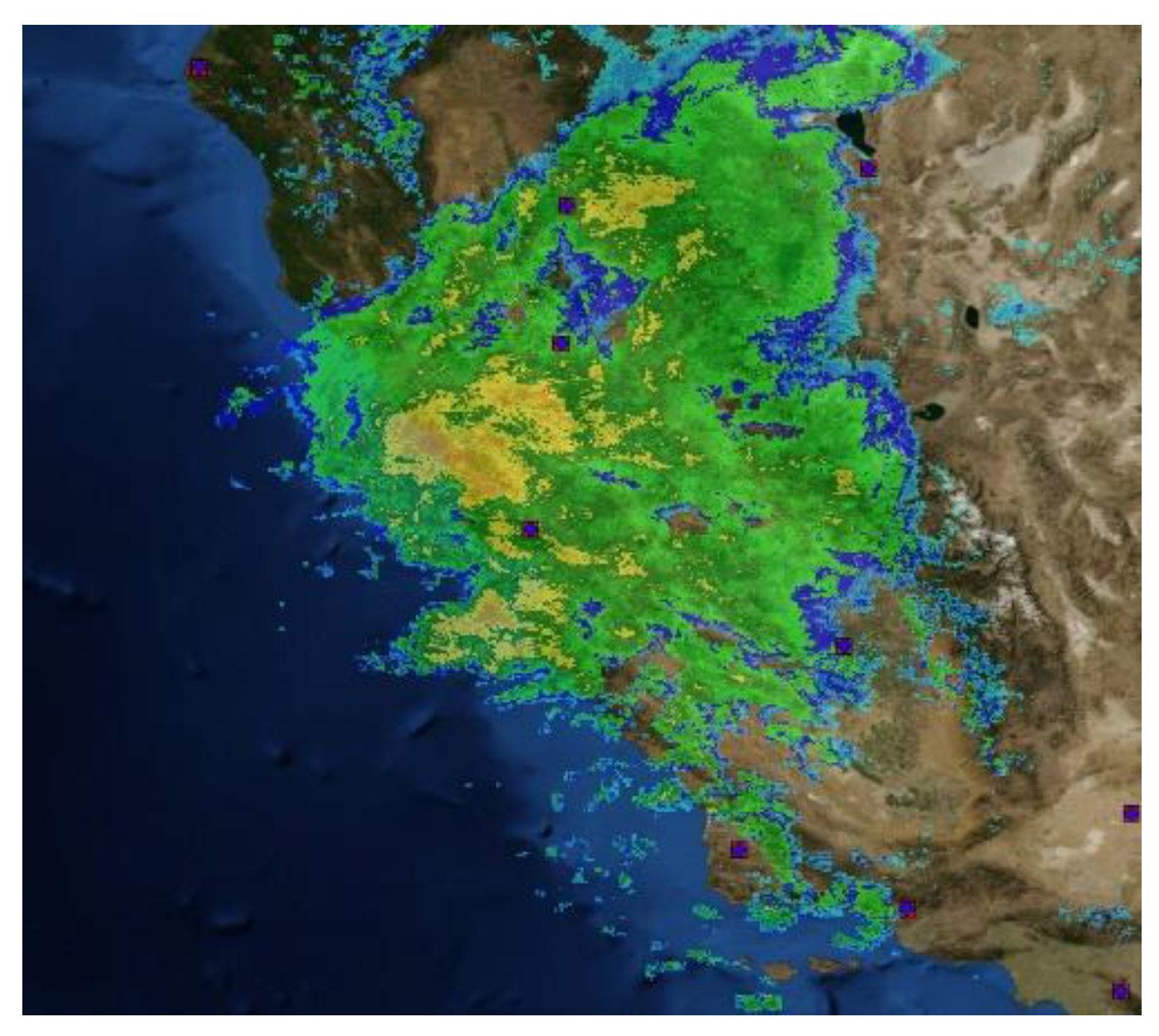
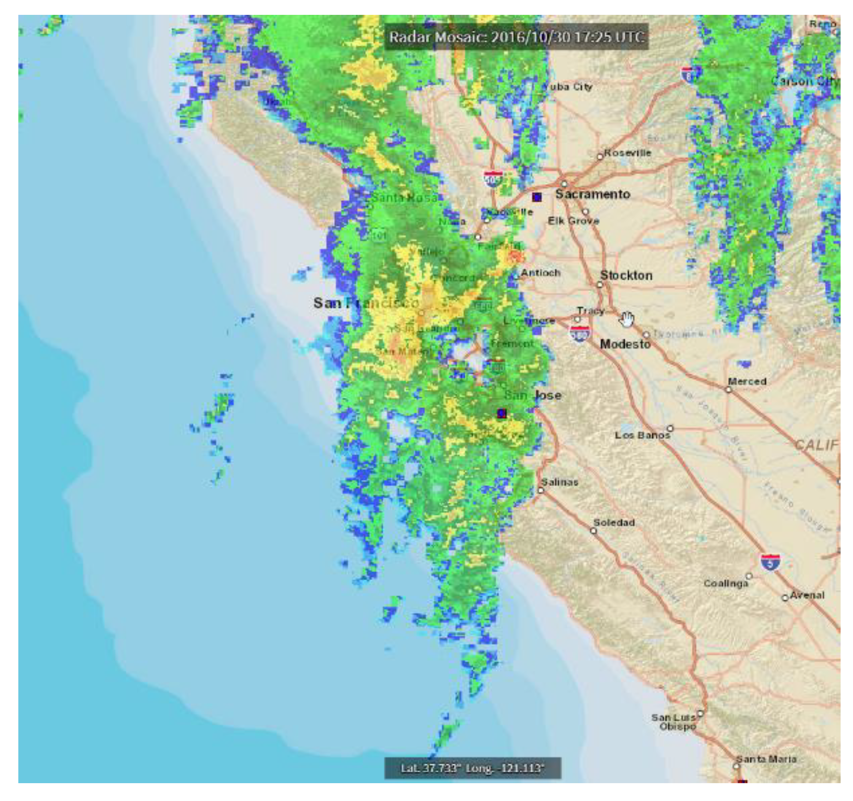
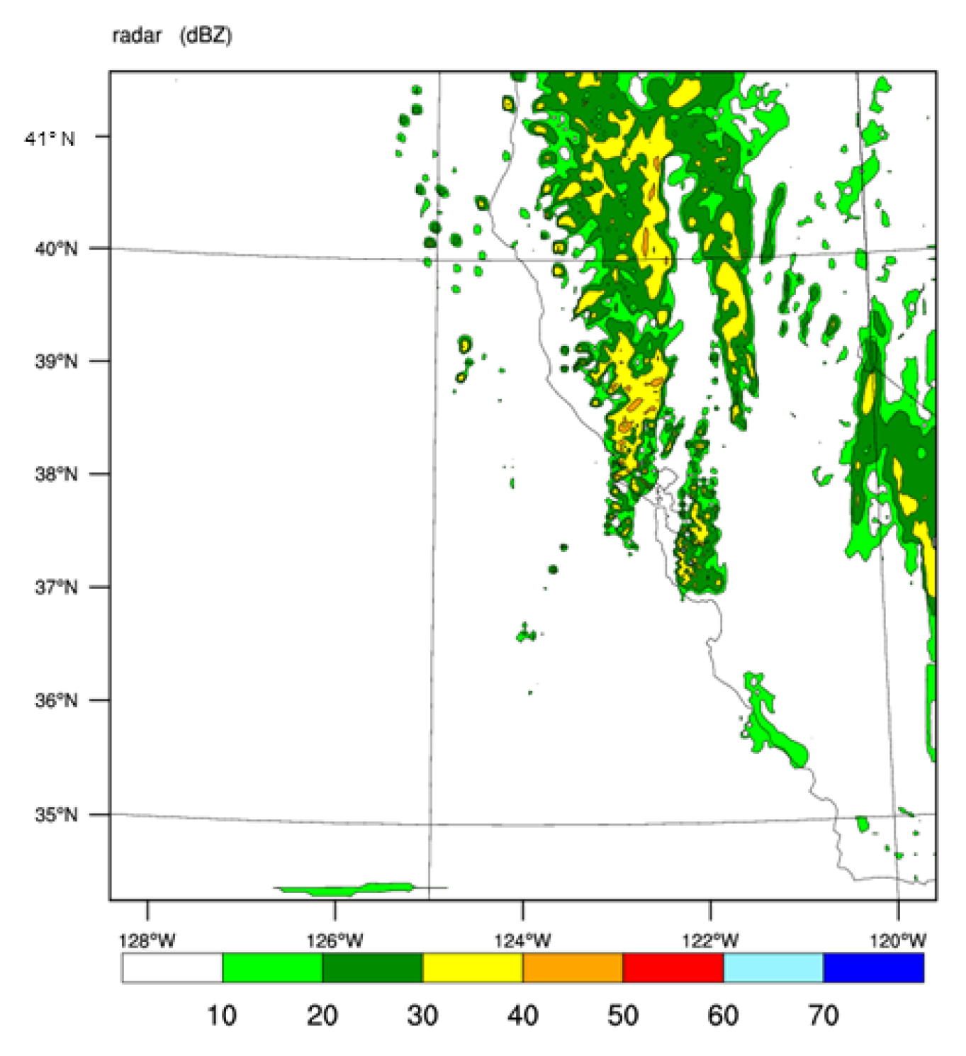
Archived radar imagery [
16] at 1055Z on 20 February (
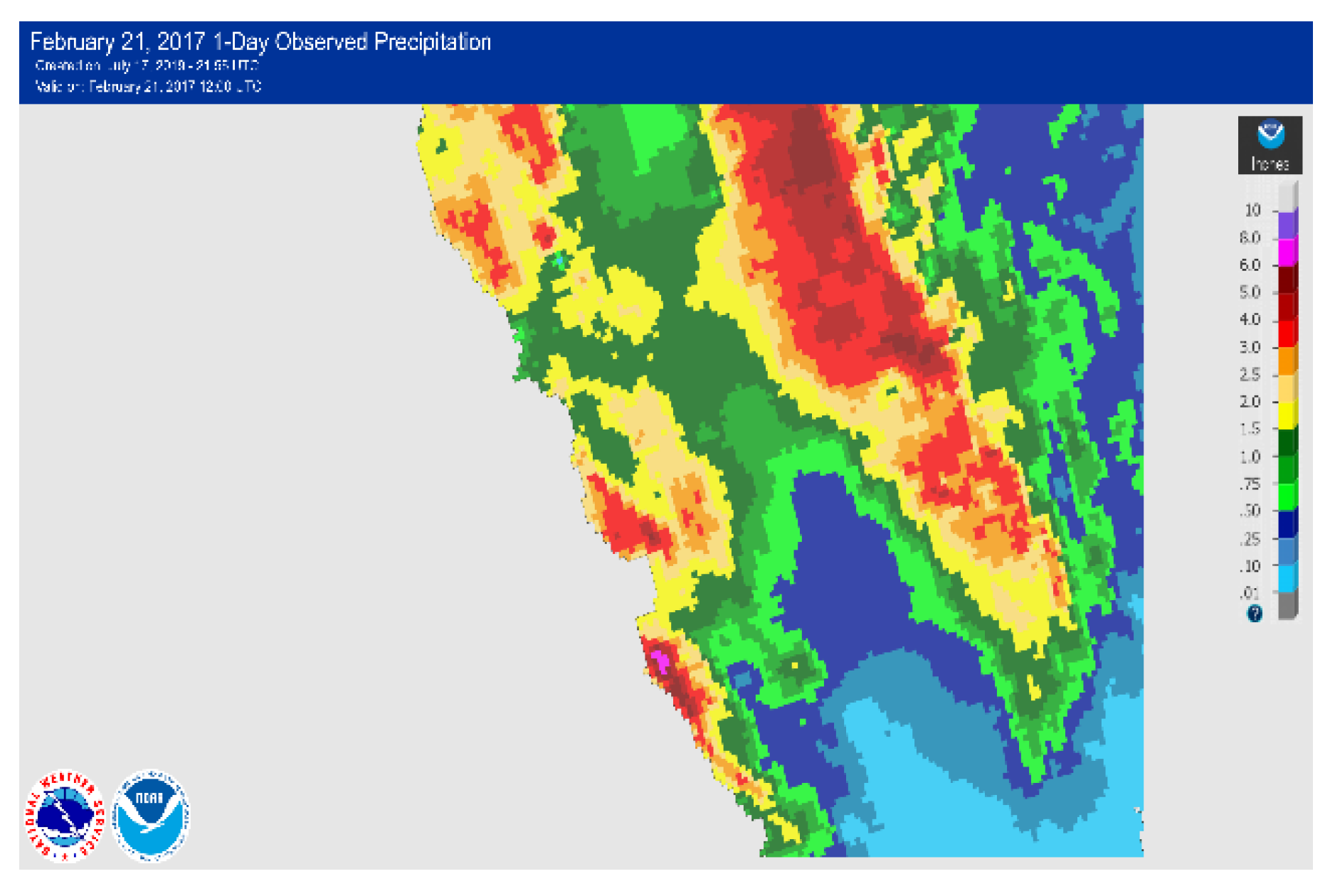
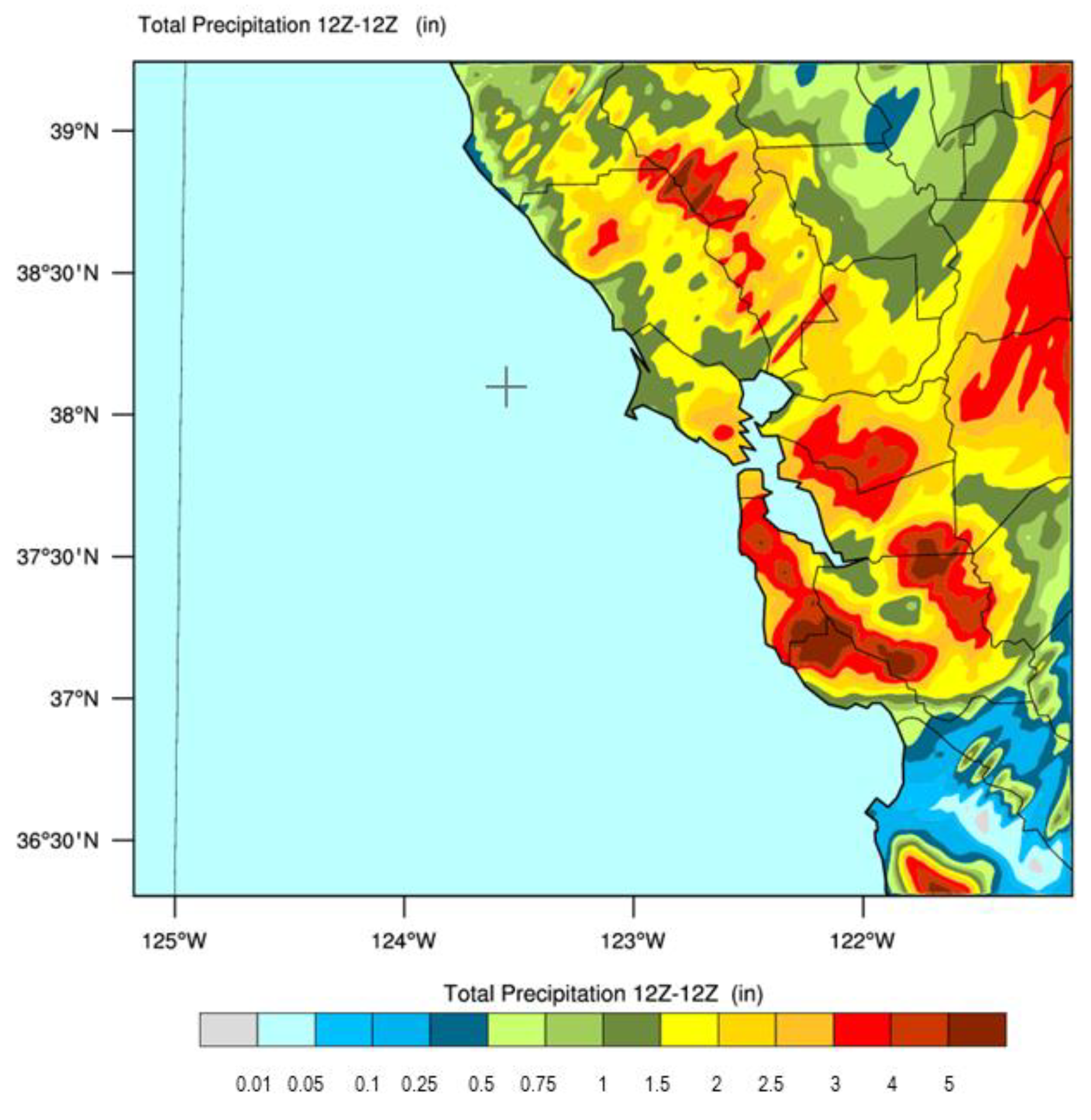
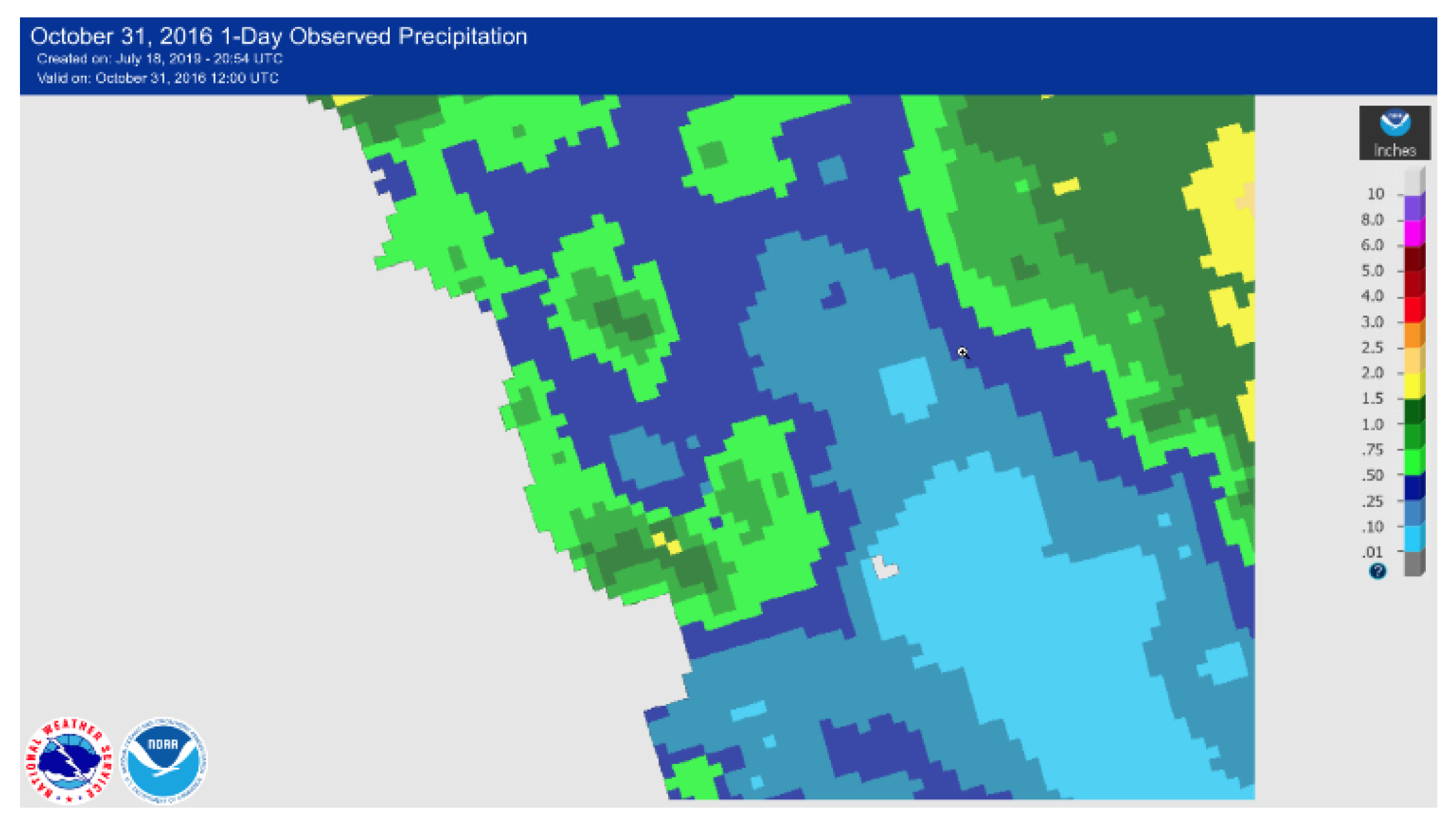
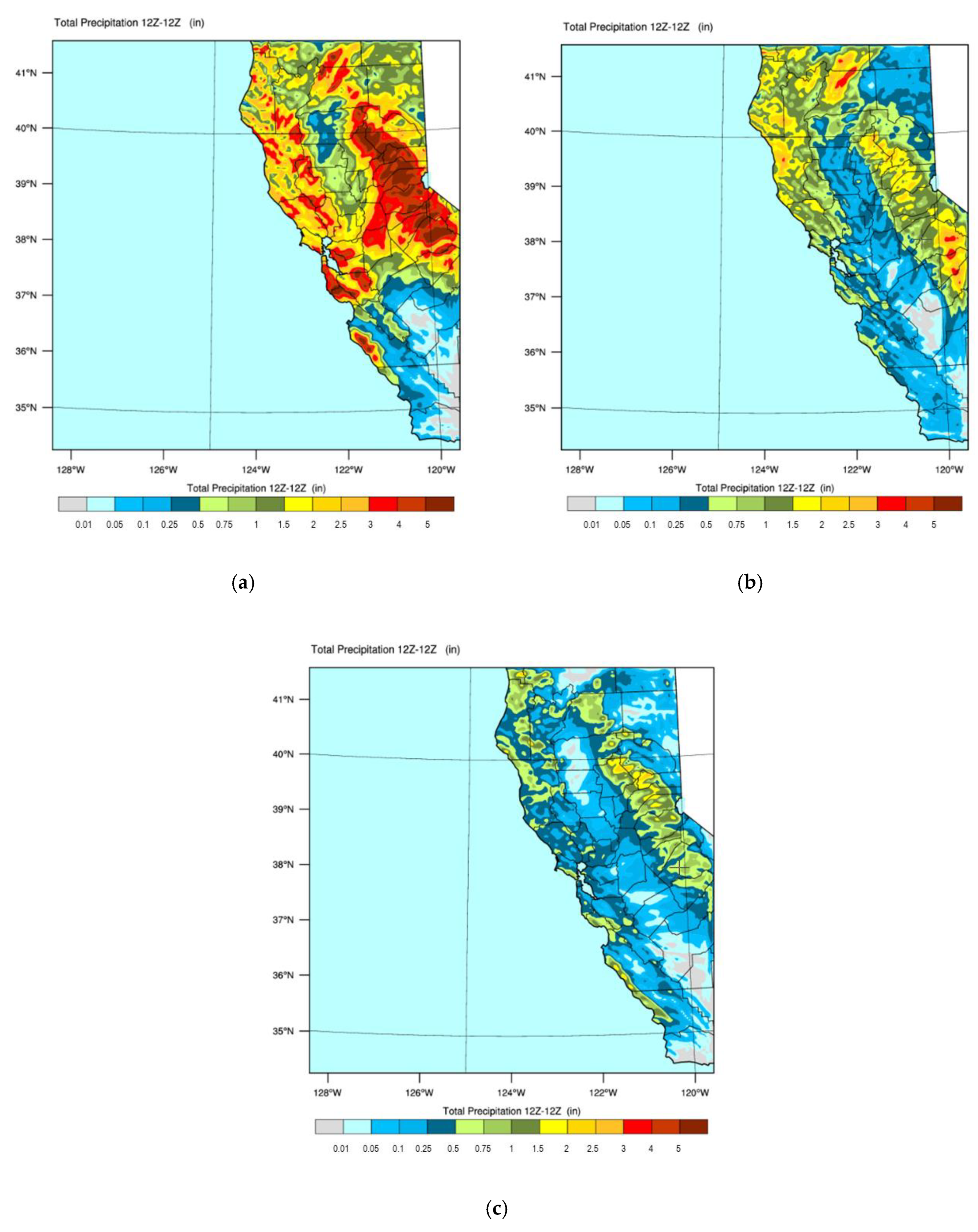
Figure 2) indicates widespread moderate rainfall was occurring at the time from about Big Sur north to the northern end of the SFBA. The total rainfall received in the region from 12Z on 20 February to 12Z on 21 February is shown in
Figure 3. This advanced hydrologic prediction service (AHPS) product [
17] combines observations and radar-estimated rainfall, binned to a 4 km resolution. Over 3” was received in many locations (North Bay, Santa Cruz mountains, Big Sur, Sierra foothills), with over 5” in several of these. Rainfall around the Bay south of San Francisco was in the 1–2” range. Although not unheard of, for San Jose to receive almost 2” of rain in a 24 h period is quite unusual. There are only three days on record with over 3” in a 24 h period [
18]. Thus, it is difficult to call this an RS event. Yet clearly, the Santa Clara Valley was rainshadowed relative to the surrounding hills.
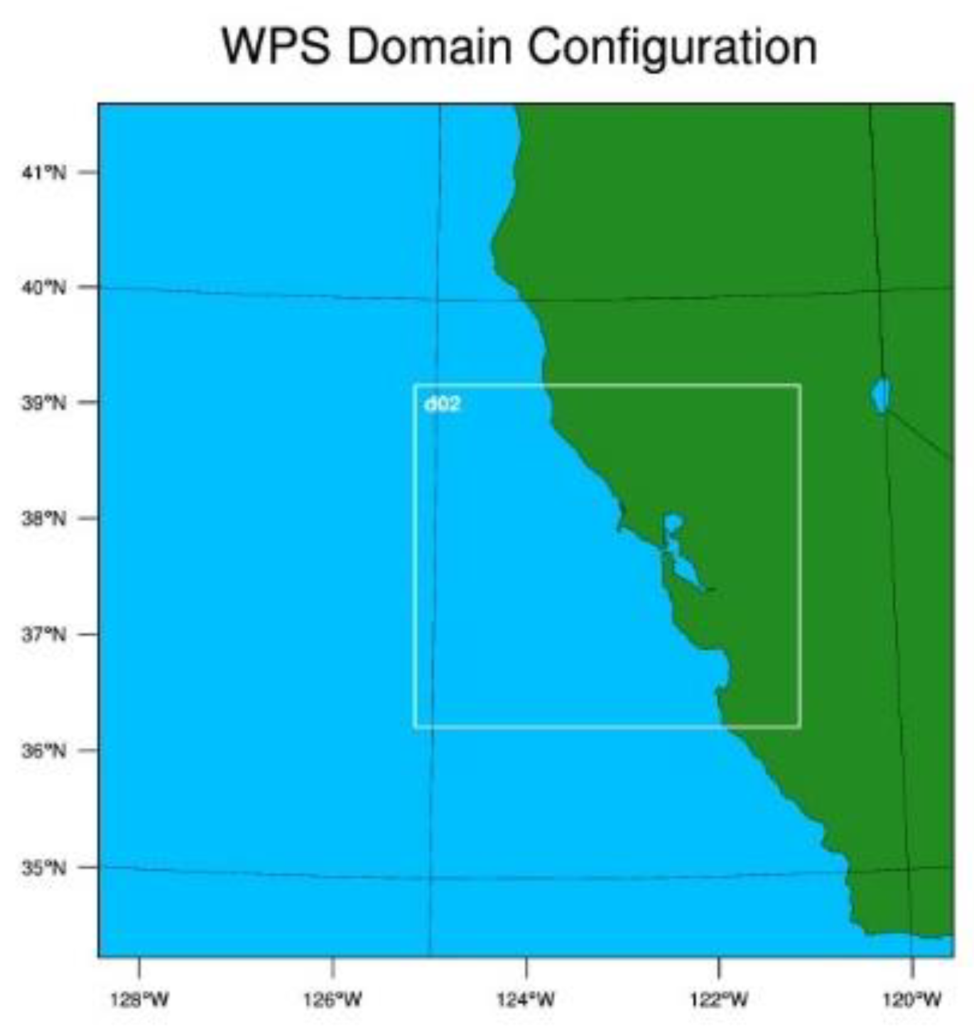
The primary goal of our study was to develop a version of the WRF model that will replicate the finer-scale details of predicted rain accumulations, and thereby allow for better prediction and planning. Local broadcast TV forecasts of rain totals tend to overestimate rain in rainshadowed locations by an order of magnitude, presumably from using coarse models like the GFS. After we examined several synoptic cases and associated WRF simulations, the configuration we iterated to has these elements: (i) GFS-driven (NAM-driven rain predictions were generally never more accurate and sometimes less accurate); (ii) two grids, the outer (201 × 201) at 4 km resolution and driven (in the experiments reported below) by GFS analysis fields, and an inner grid (271 × 241) at 3:1 ratio of 1.33 km. The comparisons were mainly focused on the outer 4 km grid. The WRF grids are shown in
Figure 4. The inner grid is offset to the west a little to better allow rain-producing elements to be simulated as they develop and move in to the SFBA from the ocean; (iii) 45 vertical levels; and (iv) physics package choices include Thompson microphysics scheme, the rapid radiative transfer model (RRTM) for the long and shortwave radiative, unified Noah land–surface model, and Mellor–Yamada–Janjic PBL scheme, (e) simulations started at 00Z and we extracted rainfall simulated in the 12Z–12Z period (36 h simulations). Some of these parameter choices (e.g., the Thompson scheme) were based on values used in the WRF model run at the local (Monterey) NWS field office, since their model is “tuned” for coastal California. Other choices were arrived at after multiple simulations (not shown) of our chosen dates, with varying parameter selections.
Each simulation starts at 00Z and we examine here only rainfall simulated in the 12Z–12Z period. We compare this to the 24 h total rainfall product produced by AHPS. Note that local NWS offices report total rainfall for local midnight–midnight, which can make precise comparisons with observations more difficult.
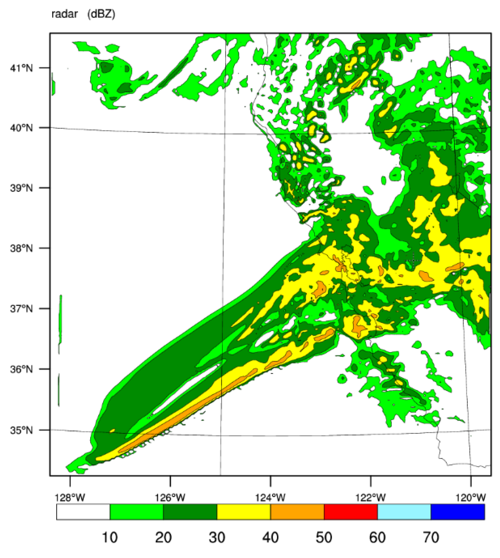
Figure 5 shows the simulated reflectivity at 1300Z from our WRF simulation of this event (using the WRF basic reflectivity product). Comparing with
Figure 2, we see echoes covering a comparable area in the north–south sense, with some higher reflectivities embedded. We also note a very sharp cutoff along the northern edge of the returns, which was also seen in the observations (which of course do not extend offshore).
Figure 6 shows the 24 h rainfall predicted over the domain. Comparing with
Figure 3, we see some good comparison with observations, including: (i) the heavier rains in the Santa Cruz mountains and Big Sur (both over 5”); (ii) the drier prediction over the Santa Clara valley, but still with widespread 1.5–2”, and even the 1.0–1.5” “hole” at about 121.8° W. Less well reproduced features include: (i) too much rain predicted in the hills east of Oakland and those just north of San Francisco; (ii) too little rain generated in the region between the SFBA and Big Sur. In both areas, errors are ~1”. As a reminder, the observed rain product (
Figure 2) is based on irregularly-spaced observations and radar-derived rainfall (in data sparse regions), all interpolated to 4 km × 4 km grid boxes. Thus, some disagreements between the WRF product and the observations may stem from comparing different rainfall products and on different grids (4 × 4 binned vs. point data). Also, in this case, rainfall distributions in some locations were sensitive to whether we looked at midnight–midnight vs. 12Z–12Z. Thus, some differences between model and observations may stem from timing on the passage of embedded higher rain-rate elements. Additional discrepancies are assumed to be associated with the schemes used to parameterize cloud and precipitation processes. Once we had settled on the “best” domain configuration for our experiments, we conducted a number of simulations with differing physics options, with a focus on radiation (the “lw” and “sw” parameters), cloud microphysics (“mp”), and cumulus parameterization (“cu”). Many wintertime cold frontal passages in Northern California are followed by the development of cumulonimbus and showers over the ocean which move onshore and provide post-frontal rain. We therefore focused on the physics packages most related to this situation (and ignored things like soil moisture etc.). Modifications to all of these parameters produced only minor changes to the forecast rain.
For the San Jose region in the southern SCV, this was a significant rain event. For a number of reasons, including saturated land from recent rains and releases upstream from the Anderson reservoir south of San Jose, a significant flooding event developed along the Coyote Creek leading to evacuations of 14,000 citizens and damage estimated at over
$100 million [
19]. The flooding took local authorities by surprise, which means that there is certainly room for improvement of local rain forecasts. The heavy rains in this event were associated with a moderate AR event. These are characterized by having a southwesterly fetch of relatively warm, moist air.
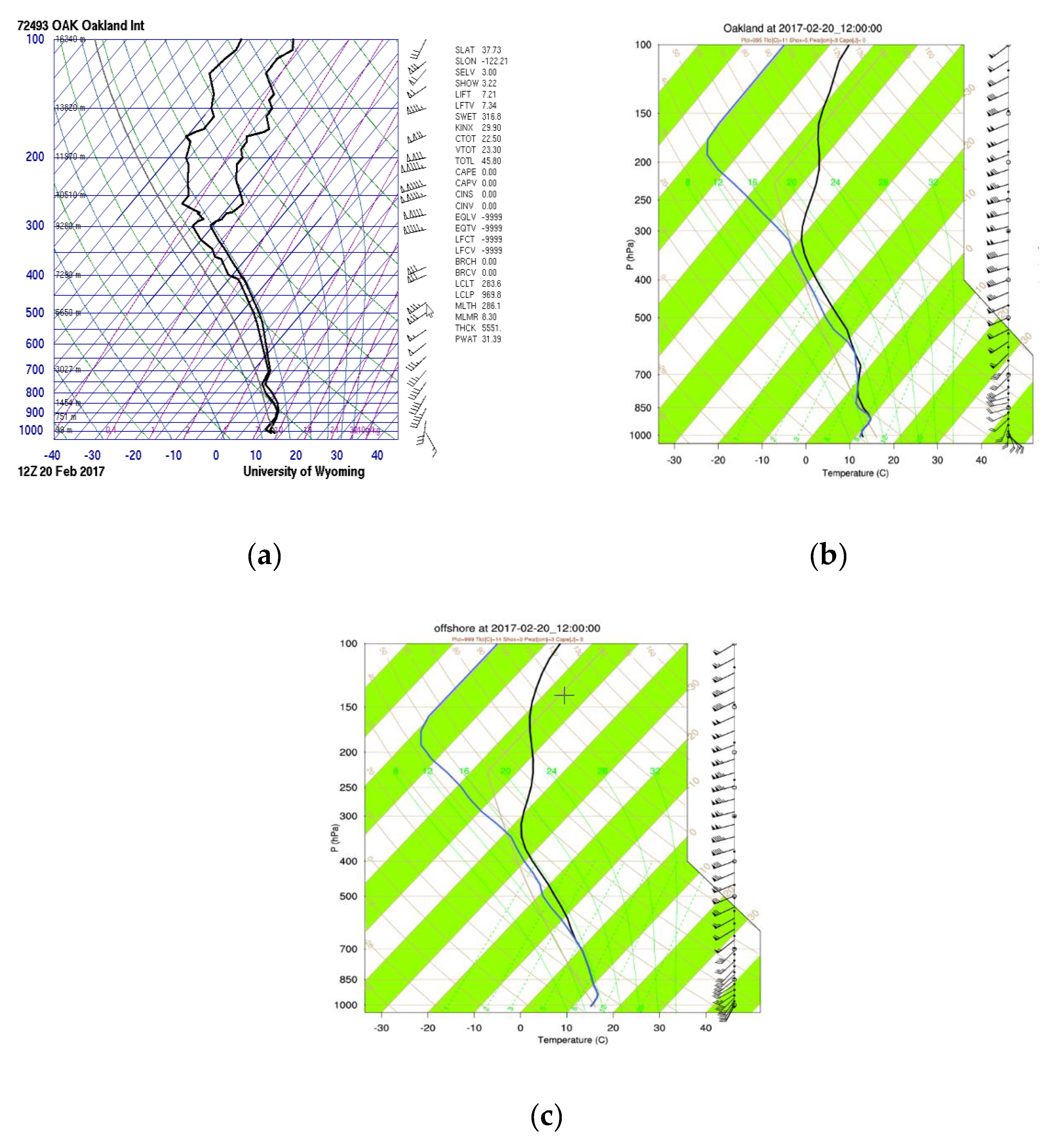
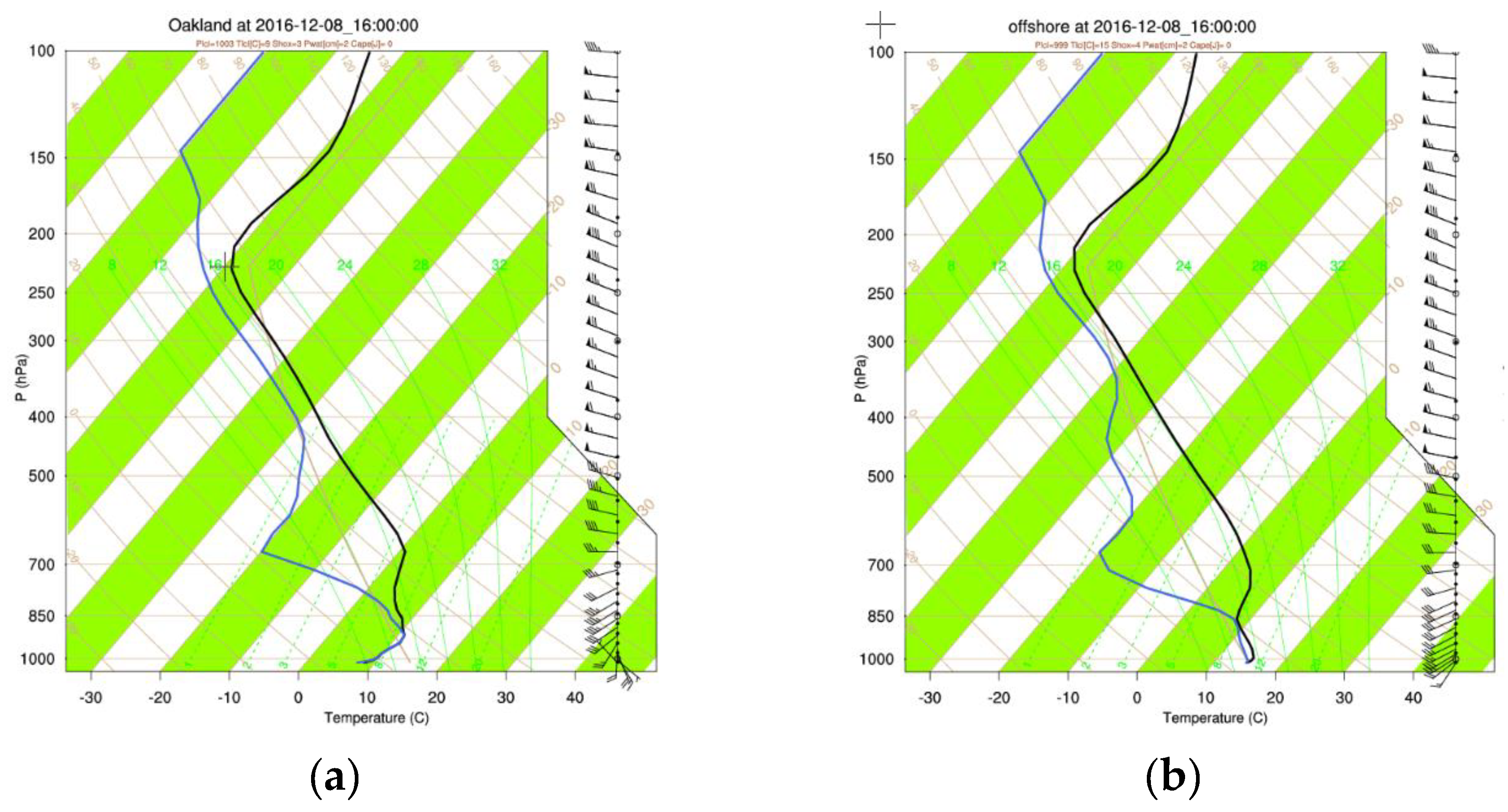
Figure 7 shows three soundings from the period: the 12Z OAK observed sounding; a sounding from the WRF simulation at WRF’s “Oakland” location (nearest grid point) for comparison; and a second WRF sounding at a location to the southwest out over the ocean (and thus away from terrain influences). All soundings indicate a very deep layer of moisture, with near saturation to ~300 hPa, and PWAT values over 3 cm. None of the simulated soundings in this event indicated any convective available potential energy (CAPE). Other events we have examined (e.g., 30 October below) do show enough CAPE to generate post-frontal showers. On 20 February, winds at all levels in the lower atmosphere were from the SW quadrant, with weak veering with height. The lowest-level southeasterly winds at Oakland (
Figure 7a,b) result from terrain influences, since they are absent offshore (
Figure 7c). Thus, with a deep layer of southwesterly flow impinging on the coastal hills with their NW–SE orientation, a strong RS would be expected if only wind directions matter in generating the RS. Clearly, however, there are other factors, since SJ received almost 2” of rain. Considering the cloud microphysics and precipitation processes,
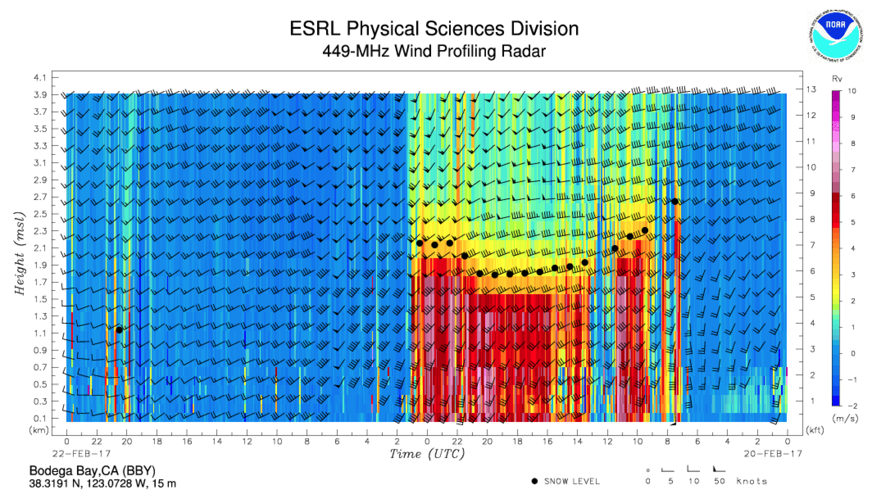
Figure 8 shows the signature of this AR storm as recorded by the wind profiling 449 MHz radar located at Bodega Bay just north of San Francisco on the coast [
20]. The black dots indicate the altitude at which snow is detected, indicating that a BB level was present and in the range 1400–2000 m above ground level (AGL; the freezing level (FZL) shown on the soundings in
Figure 7 was around 700 hPa ~3 km). Hence, frozen precipitation processes were involved in producing rain within this AR, and these typically produce higher rain rates and more rain (all else being equal [
12]). Assuming the same was true a little further south and running over the SFBA, this together with the very deep moisture layer and attendant synoptic dynamics, created significant rainfall, even in the usual RS regions.
4.2. 30–31 October 2016
Our second case study involves a synoptic situation, which is the most common rain producer in the SFBA. This involves an occluding low pressure to the NW of SF over the ocean, and rain associated with the passage of the CF. Especially in the colder months, there are typically post-frontal showers producing more rain. At 18Z on 30 October 2016, a surface low analyzed at 996 hPa was located just off the Oregon coast, with a CF that was draped to the SSW [
15]. During the day, the CF approached the coast and produced rain [
15,
16].
Figure 9 shows observed radar reflectivity at 1725Z at which time the front was draped from SSW–NNE over the SFBA, with individual rain elements running along the front from SSW–NNE. The implied rain region is relatively narrow across the front.
Figure 10 shows simulated reflectivity at 1800Z from the WRF simulation of this event. The simulation captures the observed quite well, including, arguably, the presence of two lines of activity roughly 50–100 km apart.
Figure 11 and
Figure 12 show observed and simulated 24 h rain from the event. Compared to the 20 February 2017 event, this was much less spectacular, but also more normal. Up to 1.5–2” was recorded in the Santa Cruz mountains and in the far North Bay. Lower elevations received under 0.5”, with the SCV getting 0.1–0.25”. The simulation shows a broadly similar distribution, although: (i) rain amounts in the hills were generally too low (Santa Cruz mountains north to San Mateo and San Francisco, and the east bay hills including those east of Oakland), while; (ii) the observed RS in the SCV was not sharply simulated. Station observations showed SJC received 0.17” (WRF predicted 0.13”), Oakland 0.55” (0.2”), SFO 0.52” (0.17”), and Santa Cruz 0.32” (0.01”). Recall that all observed amounts are for local midnight–midnight, whereas WRF values are 12Z–12Z. In this case, the rain event in the South Bay occurred in the overlapping time window midnight −12Z, so the 24 h totals can be directly compared. Since rainfall is so difficult to predict, we focused on patterns rather than absolute amounts, and in this case, the RS in the SCV is not as well predicted as in the 20 February case. This is evident from comparing the green shaded areas in
Figure 11 and
Figure 12a showing 12Z–12Z accumulations of over 0.5”. To show that the general spatial pattern is well-predicted, we modified the “blue–green” contour levels with the result shown in
Figure 12b—the rain pattern now looks much more like the observed. In heavy rain events where flooding might result, it is obviously important to correctly predict both the total amount of rain (and rain rate), and rain distributions. For more moderate rain events such as this (e.g., 0.25–0.75” in 24 h as is typical in the urban parts of the SFBA), a 100% error is more tolerable in terms of planning for impacts.
Winds in the 0–2 h time period leading up to the time of frontal passage were from the WSW, aligned almost perpendicular to the SFBA ridgelines, as with the 20 February case.
Figure 13 shows a pair of model soundings at 16 Z (same location as in the February case), and these indicate very little direction shear in the layer to 500 hPa at this time. Thus, the flow impinging on the coastal terrain was roughly perpendicular to the slope at all elevations. The simulated soundings also show that the moisture layer was much shallower than in the 20 February AR case discussed above. Saturation was noted up to ~600 hPa offshore at the start of the 1Z–12Z period, and above “Oakland” at 16Z as the CF progressed onshore. Wind profiler observations at this time show a BB level was located between 1.8 and 2.5 km AGL for a period of about 3 h as the front passed. Thus, frozen precipitation processes would have existed from this level up to only ~600 hPa (~4.5 km), with liquid precipitation below. With a depth of only ~2 km within which frozen precipitation processes could contribute to rainfall, it is no surprise that the October event generated much less rain than the February AR event. Finally, the simulated soundings showed that at 16Z, sufficient CAPE was present to allow convection to form, with ~430 J/kg in the post-frontal offshore atmosphere at 16Z, and ~680 J/kg at “Oakland” at 20Z (not shown). Off the California coast following winter cold frontal passages, CAPE values need only be above ~400 J/kg to support the development of showers, with higher values leading to more intense convection, some of which can become heavy rain and small hail producers. Thus, based on the simulated lower-level winds directions and thermodynamics, it was anticipated that a fairly strong RS associated with frontal rains, followed by more spatially “hit or miss” shower activity post-frontal, lead to a spatial rainfall pattern reflecting both contributions.
4.3. 8–9 December 2016
Our third case involves an event in which virtually zero rain was measured at SJC (0.01”), while zero (0.5”) was recorded in all surrounding directions (OAK, SFO, Santa Cruz)—a true rain shadow. In a typical year, the central California coastal region sees 1–2 AR storms, and 2–4 of these “no rain at SJC” storms, with the rest of the annual rain coming from storms like that on 30 October. The period examined is 12Z on 8 December 2016 to 12Z on 9 December. The surface analyses at the start of the period [
16] shows a weak surface low (1005 hPa) located offshore from the California–Oregon border, with an occluded front extending down to the SFBA, a warm front further south along the coast, and a cold front offshore. Archived radar reflectivity [
15] shows nothing on the 8th or 9th, and yet it certainly did rain on both days (SFO received 1.32” on the 8th and 0.04” on the 9th; for OAK 0.5” and 0.09”; SJC 0.01” and a trace on these days). The KMUX radar was verified to have been operational on these dates [
21]. In the SFBA, the NWS–KMUX radar is located atop Mt. Umunhum to the south of SJC at an altitude of just over 1 km above mean sea level (MSL). The radar beam is tilted upwards (+0.5° tilt) and is known to overshoot low rain clouds, especially in lighter rain events (and thus show zero echoes). It seems likely therefore that this was a fairly “shallow” rain event with mainly warm cloud physics processes in play.
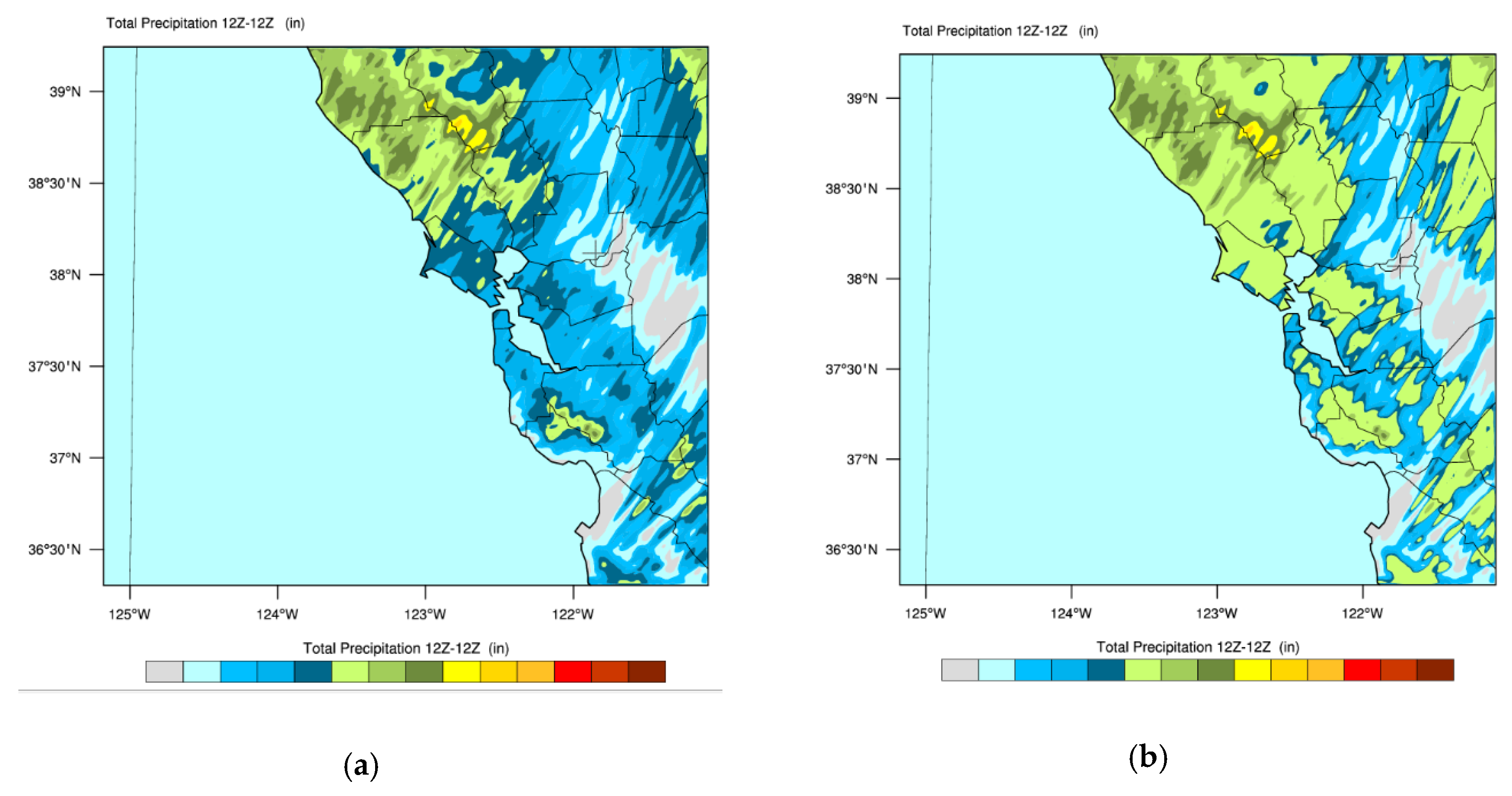
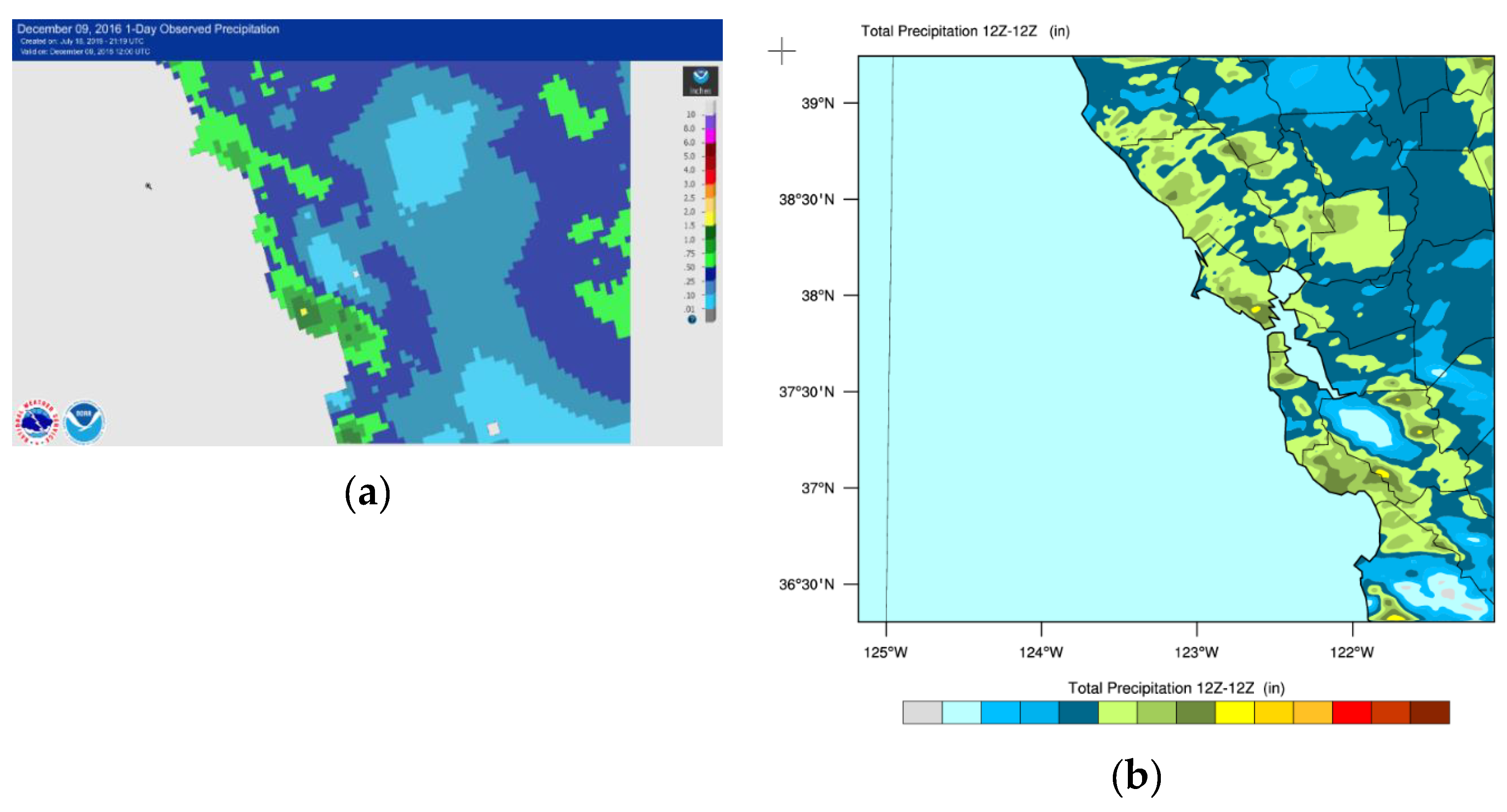
Figure 14a shows the observed 12Z–12Z rain from this event, and
Figure 14b shows the WRF-simulated rain. Observed rain totals were relatively low thought the SFBA, although a few locations in the SC mountains received around 2” in the midnight–midnight period on the 8th (per NWS–MTR climate data). Recall that the observed product (
Figure 14a) smooths this point data via 4 km binning. Most interestingly, in terms of rain shadows, the SCV received virtually no rain from this storm (0.01” at SJC, 0.04” at Moffett federal airfield). Our WRF simulation succeeded in replicating this strong RS feature (
Figure 14b), with a significant region receiving under 0.01” rain in the 12Z–12Z period. The hills surrounding the SCV received 0.5–1.5” in the simulation, with a few spots receiving up to 2”. The WRF simulation appears to have produced a little too much rain in the east bay hills (e.g., due east of SJ). However, observations in this region are sparse. What few observations are available max out at around 0.5”.
WRF-simulated radar (not shown) suggests that the main rain band passed SFO towards the start of the 12Z–12Z period. Soundings at 15Z are shown in
Figure 15. The offshore atmosphere is saturated to only 850 hPa, while inland saturation extends to about 100 hPa higher, with a strong inversion above. No CAPE is evident. Thus, this case features a shallow layer of moisture and relatively shallow clouds, which fits in with the lack of radar reflectivity from KMUX. With such shallow clouds we would expect little in the way of rain generated by ice processes, since the FZL is around cloud top (around 2 km depending on location offshore or onshore). Not unexpectedly, little in the way of a BB was seen in the Bodega Bay profiler data [
20]. In the period 8 December 2016 12Z to 9 December 2016 12Z, there was only one such report at an altitude of 393 m MSL.
4.4. Comparisons and Dynamics of the Three Cases
All three cases involved offshore winds (i.e., away from terrain influences) blowing from the southwesterly quadrant through the lower half of the atmosphere, and thus more or less perpendicular to the SFBA terrain. It appears that each event would have had some degree of RS. During the wettest event (20 February 2017), almost 2” rain fell at SJC in 24 h, not quite a record, but nevertheless a heavy rain event by local standards. It is difficult to call this a true RS event therefore, although some locations in the SC mountains to the southwest received over 6”. Our WRF simulation did well at resolving this RS, or more properly, the geographical variation in accumulated rain (over 5” in the SC mountains, 1.5–2” in the SCV). During the moderate rain event (30 October 2016), our simulation again did well at replicating the pattern, which is the main focus of this work. While rain totals in the SCV were reproduced quite well, the simulation produced too little rain in the surrounding hills. Although it should be possible to tweak physics parameters to get a better reproduction of this, our desire was to iterate to a version of WRF which worked “best” for “most” cases. In this case, since rainfall amounts were not excessive anywhere (no local reports over 1.7”), any low forecast of rain should not have impacted local planning issues. In the driest case (8 December 2016), the RS in the SCV was very well-predicted, including virtually zero rain at SJC.
What led to the differing rain amounts being measured at SJC on these three occasions, from 1.86” on 20 February, to 0.17” on 30 October, and 0.02” on 8 December? Understanding broad conditions that support weaker or stronger rain-production in the SFBA will assist us in producing forecasts that improve upon the skill of coarser-grid models. Considering first thermodynamic factors, an obvious difference between the cases was the depth of moisture associated with the synoptic events, each of which had a cold front oriented roughly parallel to the coast. The 20 February case involved a landfalling AR (moderate per [
5]), with relatively warm temperatures and a deep moisture plume. Soundings (
Figure 7) indicate that clouds would have extended to ~300 hPa, allowing a deep layer of rain formation via ice processes, since the FZL was at about 700 hPa. The multiple bright band observations from Bodega Bay support this. So, although the SC mountains squeezed moisture out of the plume, there was still plenty available to rain out over the SCV aided by favorable upper-level rain-production mechanisms. The 20 October case involved a shallower layer of moisture with cloud tops around 600 hPa. This would have allowed for less depth of rain production via frozen processes, and thus less rain, all else being equal. The driest case (8 December) had the shallowest moisture plume and very little evidence of ice processes in rain production, and thus least rain.
Turning to dynamical factors that could explain the differing rain amounts, our only attention thus far has been on the lower atmospheric winds as they impacted the SC mountains. No doubt stronger/weaker dynamical factors associated with each case could have added to overall rainfall via synoptic-scale vertical winds, as well as updrafts in convective elements embedded in the flow. Looking at some “dynamic” elements with each case, we note the following:
- (a)
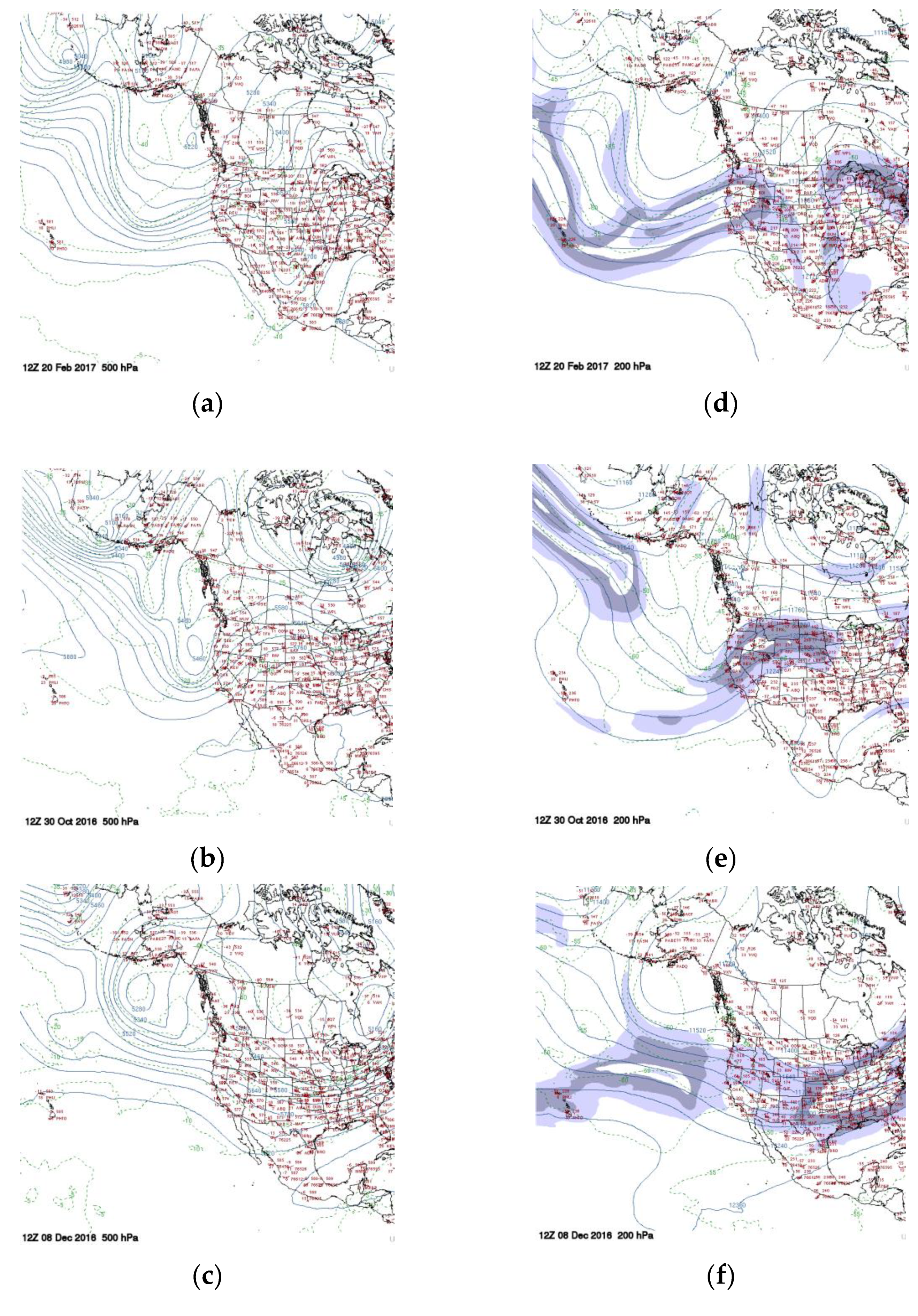
Heights at 500 and 250 hPa over the Pacific for the three cases are shown in
Figure 16. At 12Z on 20 February (
Figure 16a), a deep 500 hPa trough was located well offshore, with heights of ~5380 dm located well west of OAK at ~141° W (500 and 250 hPa maps from the University of Wyoming online archive [
22]). At 12Z on 30 October 30 (
Figure 16b) a weaker trough (heights ~5500 dm) was located closer to the coast (axis at ~128° W). In both cases, the thermal trough was collocated with the height trough. At 12Z on 8 December (
Figure 16c), a closed low of 5280 dm was located in the Gulf of Alaska just east of the Aleutians. However, the west coast was under a weak 500 hPa ridge—not an ideal synoptic situation for rain in the SFBA.
- (b)
At the 250 hPa level on 20 February (
Figure 16d), the jet was oriented SW–NE over California with its axis of peak winds north of OAK and the SFBA under the “right-front” segment of the jet. A broadly similarly jet arrangement existed on 30 October (
Figure 16e), with the jet axis over the SFBA and the “right-rear” segment well south of the SFBA. On 8 December (
Figure 16f), a jet streak was noted west of the SFBA, but too far offshore to support additional synoptic-scale uplift. Thus, synoptic enhancement to lift associated with jet quadrants was not present in any of our cases.
- (c)
Observed wind speeds at 500 hPa from the Oakland sounding ranged from 71 kts at 12Z on 20 February, to 67 kts on 30 October, to 48 kts on 8 December. In the February sounding, there is evidence of a low-level jet (LLJ) with speeds peaking at 43 kts at 874 hPa. No evidence of an LLJ is seen in the other two cases. The interaction of this LLJ with the SC mountains (and other ranges) undoubtedly enhanced uplift and precipitation there.
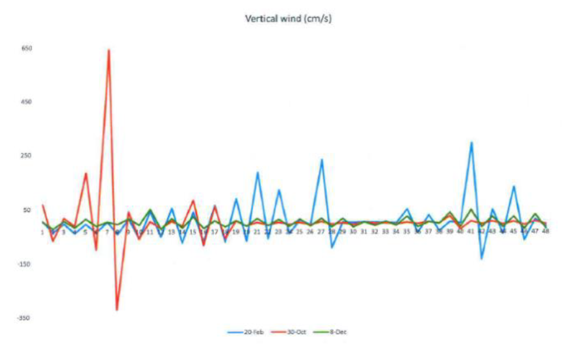
- (d)
Vertical winds are not measured, but can be extracted from our WRF runs. Across a 10 × 10 grid box just west of SF over the ocean, the maximum instantaneous upward and downward wind speeds were extracted at every hour through each simulation, and these are shown in
Figure 17. Maximum upward wind speeds are weakest in the December case (green line), which fits in with the general weakness of that event. In the October case (red), we see the passage of the front 3–4 h into the period, and associated strong uplift with weaker vertical winds thereafter. Finally, in the February case (blue), there is a suggestion of a couple of stronger impulses moving through (around 13 and 20 h into the period), which might suggest “bursts” of heavier rain embedded in the general rainy pattern.
In summary therefore, clearly the 8 Dec case was synoptically weakest and also had the shallowest layer of moisture available to wring out. It is not surprising therefore that SJC received almost zero rain in this true RS event. Our WRF run replicated this very well. In many respects, the October event was synoptically strongest in terms of the proximity to the upper-level trough and the strength of vertical winds simulated just offshore with frontal passage. The synoptic arrangement was certainly not conducive to a heavy rain event, since the jet core was directly overhead, the offshore trough was vertically stacked, and only the lowest 400 hPa at best of the atmosphere was saturated. Air behind the front was not particularly cold so only low amounts of CAPE developed, and thus post-frontal showers were few and relatively light. Finally, in the February case, there was a deep trough, but it was located quite far offshore. Hence, the SFBA was under the influence of a southwesterly flow of very moist air (PWAT at OAK over 3 cm) associated with the moderate AR event. With saturation to ~300 hPa, terrain-induced lifting of this moist airmass as it impacted the SC mountains would have produced rain in upwind areas, enhanced by the LLJ. However mesoscale- or synoptic-scale lift would have been needed to generate rain downwind in RS regions. The vertical winds, in this case, were weaker than in the October case, but the combination with plentiful moisture led to widespread significant (and flooding) rains. Also, in this case, the axis of the AR stayed in place for about 24 h, allowing significant accumulations (by local standards). Based on these comparisons, we suggest that future weak synoptic events with a shallow moisture source would have difficulty in generating any rain in the SCV. With deeper moisture there would be a little more rain, but hardly anything noteworthy from a flooding perspective. SJC might receive 0.25”–0.5” in such cases. The only arrangement that is likely to lead to flooding is an AR event, as previously noted [
5].
4.5. Lower Resolution Simulations
To determine the extent to which high-resolution needs to be used to get a good RS simulation/prediction, the sensitivity test was conducted with only the outer (4 km) grid (
Figure 18a–c). Focusing on the southern part of the SFBA, the RS is not as pronounced in the February case as with the 1.33 km nested grid (compare
Figure 18a and
Figure 6). The rainfall totals in the surrounding hills all look about the same, but the local minimum in the SCV is not as sharply defined. In the October case, the high-resolution simulation was deficient in rainfall in the SC mountains, but with a single grid, rainfall in the hills is enhanced (
Figure 18b). This is true both west and east of the SCV. Finally, in the December case, the one domain result seems noticeably worse (
Figure 18c). Too little rain was predicted along the peninsula from the SC mountains north to San Francisco, as well as in the hills east of the SCV. Meanwhile, too much rain was predicted over the SCV, resulting in a poor representation of the observed RS on that date.
Thus, since two of our three events are better simulated (in terms of the RS in the SCV) using the 1.33 km domain focused over the region of interest, we would choose to operationalize with the higher resolution.
5. Conclusions
Rain in the SFBA results from a number of synoptic circumstances. In almost all of these, the SCV is in a rain shadow, and often receives much less than forecast by local TV stations and models, such as the GFS. Our main goal in this study was to develop a version of the WRF model that predicts these local rainfall distributions more accurately. As a secondary goal, we examined possible causes for observed variations of total rain and the likelihood that WRF could accurately simulate these. Cases we examined include: (1) a very typical case in which the southern end of a CF passes through, generating a short period of moderate rain, followed by a few showers. This type of synoptic event generates a significant portion of the annual rain in the SFBA; (2) a subset of the above in which the heart of the SCV received effectively no rain, while surrounding stations received zero (1/2”), a complete rain shadow; and (3) a less typical case of an AR centered on the SFBA which produced widespread relatively high rain amounts, including in the SCV. As we mentioned earlier, no two rain-producing events are identical—our study was aimed at developing a configuration of WRF which can successfully predict characteristics of each of the three case study storms, with the expectation that any successes will be replicated in similar synoptic events.
Our simulations successfully captured the observed patterns of 24 h rainfall well, especially in the southern end of the SFBA centered on the SCV. In the driest case (8 December 2016), based on our simulation, we would have predicted under 0.05” of rain in this region (SJC reported 0.01”). In the wettest case (20 February 2017), the simulation predicted 1.5–2” of rain across a region where such amounts were observed (SJC 1.87”), and where flooding resulted. At the same time, both simulations captured elements of what was observed in surrounding locations, including: (i) higher rain amounts in the SC mountains and northward towards SF; and (ii) higher rain amounts in the mountains east of the SCV. In the February case, rain amounts north and east of SF were over-predicted (e.g., in the range 3–4” as opposed to the observed 2–2.5”). Since this was an AR event, the exact positioning of the core of the AR can have a huge impact on local rainfall and on north–south gradients of rainfall. Recall that an AR is over 1000 km in extent along the axis, but much narrower across the axis. The “point of contact” with the coastline can remain unchanged for multiple hours (often leading to flooding rains) but can also “wobble” in a north–south sense, and this location predictability still presents problems for large-scale models such as GFS and NAM. No doubt the lack of surface observations offshore hampers accurate forecasting. AR location information is ultimately provided to WRF from the GFS model (in this study) which provides initial and boundary conditions for the simulation. The extent to which the GFS model accurately predicts the location of the core of the AR will therefore impact our rainfall predictions.
The spatial distribution of rain was also quite well simulated in the 20 October case, but overall, amounts were too low in the surrounding hills. Factors which could account for this include: (i) too little moisture (in the form of precipitable water) in the impinging air mass and/or the moist layer being too shallow; (ii) a shortcoming of the microphysics packages used in these simulations; or (iii) insufficient lift of the air to induce condensation and formation of precipitation. This could, in turn, result from offshore horizontal flow being too weak, leading to weak upslope flow in the coastal mountains. It could also result from the overall synoptic disturbance, as realized by the surface front and/or the upper-level divergence field, being too weak in the simulation. It would be challenging to tease out which of these was the cause of the low rainfall in this case.
Comparing the three cases, some better simulations of local rainfall patterns were obtained using higher resolution (1.33 km here). The experiments with 4 km resolution were very broadly similar, but lacked the detail in the southern SFBA. Hence, in operationalizing we would use the 1.33 km resolution. The operational HRRR model uses a 3 km resolution, so would be expected to get some, but not all, of the spatial detail of the SFBA.
The wettest storm (20 February) had by far the deepest moisture plume, with saturation extending through the depth of the troposphere. Although a relatively warm storm (since AR plumes extend back to the subtropics), clouds were deep enough that significant rain production through ice processes was present. This is evidenced by BB data from Bodega Bay (
Figure 8), which showed a deep layer of saturation above the BB level. At the opposite end of the spectrum, the 8 December case had essentially zero rain in the SCV, a true local rain shadow. This was also the event with the shallowest moisture layer, and very little BB activity. Indeed, the event was so shallow that the local KMUX radar beam overshot and showed no echoes. Comparing these two events, it is tempting to conclude that the main factor that determines the strength of the RS in the SCV is simply the depth of the moisture layer associated with the storm, but the atmosphere is rarely that simple. Finally, when planning for winter rain events and potential flooding, in addition to guidance from our WRF simulations, radiosonde observations from KOAK and 449 MHz radar data from Bodega Bay can provide useful guidance regarding: the depth of the incoming moisture field; the extent to which a BB level exists, indicative of ice processes at play; the prevailing wind direction relative to the large-scale terrain; the presence of a LLJ; and the stability of the atmosphere.
Although numerical forecast models have improved tremendously in the last two decades, rainfall remains one of the most challenging forecast products, in terms of timing, intensity, and amount. This is all the more true in regions of complex terrain with upslope enhancements and rainshadows. Rainfall forecasts are of great interest to the general public, as well as emergency and water managers. Our goal in this study was to seek a configuration of WRF which would give more accurate short-term forecasts of rain in the SFBA. Our focus was on the 24 h window, but could easily be extended to 48–72 h. Our WRF version produces rainfall forecasts which overlap well with observations for a range of synoptic cases chosen from the 2016–2017 rain year. We are running the model operationally in preparation for the 2019–20 rain year. Especially for the southern SFBA, we are confident it will yield useful rainfall forecast products that are more accurate—and useful—than those from the coarser models, such as the GFS, NAM, and HRRR.


