Abstract
With the great strides of China’s economic development, air pollution has become the norm that is a cause of broad adverse influence in society. The spatiotemporal patterns of sulfur dioxide (SO2) emissions are a prerequisite and an inherent characteristic for SO2 emissions to peak in China. By exploratory spatial data analysis (ESDA) and econometric approaches, this study explores the spatiotemporal characteristics of SO2 emissions and reveals how the socioeconomic determinants influence the emissions in China’s 30 provinces from 1995 to 2015. The study first identifies the overall space- and time-trend of regional SO2 emissions and then visualizes the spatiotemporal nexus between SO2 emissions and socioeconomic determinants through the ESDA method. The determinants’ impacts on the space–time variation of emissions are also confirmed and quantified through the dynamic spatial panel data model that controls for both spatial and temporal dependence, thus enabling the analysis to distinguish between the determinants’ long- and short-term spatial effects and leading to richer and novel empirical findings. The study emphasizes close spatiotemporal relationships between SO2 emissions and the socioeconomic determinants. China’s SO2 emissions variation is the multifaceted result of urbanization, foreign direct investment, industrial structure change, technological progress, and population in the short run, and it is highlighted that, in the long run, the emissions are profoundly affected by industrial structure and technology.
1. Introduction
China has been the largest developing country in the world. Since the late 1980s, it has constantly expanded its economic scale and maintained at least a 9% annual economic growth rate over three decades [1,2]. In the meantime, considerable energy resource consumption has become a substantial cost of such rapid development, and leads to a large amount of sulfur dioxide (SO2) emissions. China has inevitably appeared as a big SO2 emitter as well as the largest energy consumer in the world [3]. Despite being the second-largest economy, China has yet fulfilled its historical task, that is, urbanization as well as industrialization [4]. Therefore, China confronts the challenge of curbing atmospheric pollution emissions when maintaining rapid economic growth [5]. During the 12th Five-Year Plan (2011–2015), the central government’s goal of SO2 abatement was an 8% decrease in 2015 compared with the emission level of 2010 [6].
In the atmosphere, SO2 can directly exacerbate heart disease, result in respiratory diseases in humans, and cause acid rain after reaction with other elements [7]. Except for public health, SO2 also exerts ecological and economic effects. Owing to the rapid urbanization and industrialization process, many cities in China are affected by serious fog and haze pollution [8]. Sulfate stems from ambient SO2 and accounts for 20–35% of the atmosphere PM2.5, which leads to smog [9,10] and threatens the eco-system and economic sustainability [11]. In 2008, the SO2 pollution-related agricultural losses roughly reached $1.43 billion, which accounts for approximately 0.66% of the added agricultural output value in China [12]. China’s SO2 emission level has already exceeded the levels of the United States and summed OECD (Organization for Economic Cooperation and Development) countries [13]. It is anticipated that in China, SO2 emissions would continually increase and reach 24–31 million tons by 2020 [14]. Apparently, there is no time to delay for the SO2 mitigation under the circumstance of sustainable development.
For many years, China has been the largest country of foreign capital inflow among developing countries. The constantly injected foreign direct investment (FDI) prompts the advancements of technology and management among domestic enterprises, economic development, and international business/export trade [15]. Hence, environmental economics scholars start to focus on the influence of FDI on pollution emissions and environmental quality in China (e.g., Wang and Jin [16], Bao et al. [17], and Dean et al. [18]). Additionally, the Chinese government began to upgrade and promote the optimization of the industrial structure since 2015 for the sake of emission-reduction and energy-saving. The cross-industry transmission of production materials could influence the pollution emissions [19,20], and China’s gradually updated industrial structure is expected to be beneficial for environment in practice [21]. Furthermore, over decades, the local governments have been expanding urban and suburb areas’ infrastructure construction, attempting to sprawl the cities [22,23,24], and China is transforming from an agricultural country to a modernized one [25]. Currently, more than half of the Chinese population already lives in urban areas [26]. Meanwhile, rapid urbanization and related economic activities may promote soaring resource consumptions and air pollution emissions. In sum, the relationships of SO2 emissions to FDI, industrial adjustment, and urbanization are worthy of exploration, because a better understanding of such relationships provides a scientific basis to coordinate the economic development and reduction of SO2 emissions.
Some recent studies focused on carbon and other kinds of pollution emissions issues [27,28,29,30,31,32,33,34], whereas the studies that applied rigorous quantitative methods on the socioeconomic determinants of SO2 emissions are still scarce. Several scholars tried to unfold the spatial pattern of China’s SO2 emission in their studies. Zhao et al. [35] examined the spatial variation and driving factors of China’s industrial sulfur emissions and intensity from 2001 to 2014, and they found significant spatial clustering patterns that drastically varied over space and time. Zhou et al. [36] studied the nexus of SO2 emissions to economic development through the spatial panel data model and concluded an inversely N-shaped environmental Kuznets curve. Yang et al. [37] examined the SO2 geographical distributions through China’s 113 main cities and found the cities that were heavily polluted located in the north, while cities of low pollution level mainly agglomerated in the south. Zhao et al. [38] found that fossil fuel consumption is the major contributor of China’s SO2 discharge. Li et al. [39] studied the spatial distribution of SO2 at China’s prefecture-level. According to their results, the cities of lower SO2 concentrations clustered in the Pearl River Delta and Yangtze River Delta regions, because there were less iron and steel manufactures, non-ferrous industries, and thermal power plants in the regions. On the other hand, the cities with higher concentrations mainly located in the Loess Plateau as well as the north plain. Giacomini and Granger [40] advocated the necessity of controlling for spatial effects (e.g., spatial autocorrelation, spillover (cross-boundary) impacts) when examining the socioeconomic activities’ influence on environmental quality. Anselin [41] also argued that it is necessary to adopt the spatial measurement approaches in the environmental/resources economics research on the regional level.
These initial explorations have preliminary investigated the spatial distributions and socio-economic influential factors of SO2 emissions in China, yet scant researches to date have identified the emissions’ space–time characteristic. In addition, socioeconomic factors’ space–time effects on air pollution emissions have not been paid enough attention, and the effects need thorough examination through a proper empirical framework/approach. To this end, this paper makes efforts to complement prior researches by investigating SO2 emissions’ spatiotemporal dynamics and the determinant variables across Chinese provincial-level units through exploratory spatial data analysis (ESDA), and the dynamic spatial econometric approach that organically condenses space-units’ spatial and temporal dependence into the empirical specification. The analysis and findings would help policymakers to promulgate effective policies to reinforce the SO2 abatement and air pollution control.
The present study’s major contribution is two-fold. First, the study identifies the evolvement of SO2 emissions’ spatial distribution and association patterns over time in China using GIS techniques and spatial statistics. Second, this study quantifies the socioeconomic–SO2 spatiotemporal nexus through the recently improved dynamic spatial panel data model [42] that simultaneously integrates the spatial externalities and temporal effects. In this way, the variables’ long- and short-term impacts on the space–time dynamics of air pollution emissions are distinguished for the first time. Broadly speaking, a better realization of SO2 emissions’ relation to socio-economic activities is helpful for figuring out the potential factors of increasing sulfur emissions witnessed among Chinese provinces, how the factors affect the emissions, and for further development of targeted policies for emission reduction.
The remainder of the paper is organized as follows. Section 2 describes the variable details, data source, and methods employed within the study. Section 3 illustrates and explains the results derived by the methods presented in Section 2, and then Section 4 further discusses the results and illustrates the related theory as well as the mechanism. Section 5 sets out the conclusions and policy implications drawn from the results and findings.
2. Data and Methodology
2.1. Variables Selection and Data Resources
The following analysis adopted Chinese provincial panel data spanning from 1995 to 2015 (Taiwan is excluded owing to data unavailability) within the present study. The provincial data with relatively longer intertemporal enabled the empirical analysis to capture more spatial heterogeneity and temporal variations.
According to the subject, the following extended stochastic impacts by regression on population, affluence, and technology (STIRPAT) model serves as the theoretical benchmark for the regression analysis:
where stru, urb, and fdi refer to industrial structure, urbanization level, and foreign capital inflow, respectively. lnGDP (gross domestic product (GDP) in logarithm) together with its’ quadratic term (to capture the nonlinear environmental effects of GDP [43]) reflects the economic growth influence, while lnPOP and lnEI refer to the impacts of population and technology on the environment, respectively. The dependent variable lnSO2 represents the SO2 emissions (in logarithm) in this paper. ε is the error term. Because the studies that discuss the effects of economic development and population on SO2 emissions are saturated, this paper focused on the effects of industrial structure, technology, urbanization, and FDI.
The definitions of industrial structure (stru), foreign capital inflow (fdi), urbanization level (urb), economic growth (GDP), population (POP), and technological progress/energy efficiency (EI) [44] are listed in Table 1. The author multiplied the stru, urb, and fdi by 100, and took the logarithm of the rest of the indicators in the regression analysis (Section 4). In this case, the coefficients b1–b5 in Equation (1) can be interpreted as the ecological elasticity [45]. It is worth noting that all the variables are with their actual/raw values (not in logarithm) in the ESDA section (Section 3).

Table 1.
Definitions and descriptive statistics of the variables.
The SO2 emissions and standard coal consumptions (kg of coal equivalent) were collected from the China Energy Statistical Yearbook. The secondary industry, tertiary output, as well as FDI can be accessed from China City Statistical Yearbook in the EPS data bank. The per capita GDP, the urban, and total population were obtained from the China Statistical Yearbook. Table 1 lists definitions and descriptive statistics of all variables.
2.2. ESDA
ESDA is regarded as the preliminary exploration before suggesting determinants to influence the spatial phenomena, and prior to testifying more confirmatory empirical analysis—the spatial regression model [46]. ESDA includes the techniques and steps of spatial data investigation—detecting and visualizing distributions and patterns in terms of geography, as well as identifying spatial heterogeneity forms, for example, regional/provincial regimes.
2.2.1. Global Spatial Autocorrelation
The most popular statistics measuring global spatial autocorrelation are Global Moran’s I statistics [47] developed by Moran [48]. Global Moran’s I statistics give a formal indication of whether the distribution pattern of a spatial index is clustered, random, or dispersed. The formula of the statistics is seen as , −1 ≤ I ≤ 1, N = 30, where ; x is the index of interest (SO2 emissions in this research); and wij is the element on the i-th row and j-th column of the spatial weight matrix W. The significance of Moran’s I statistics is identified by z-statistics, with the comparison of Moran’s I and its expectation as follows: , where , , , , and . When I ≤ 0 significantly, the areas with the index of high values tend to locate near the ones with the index of low values (HL clustering); when 0 ≤ I significantly, the spatial units with the index of high values cluster together and vice versa (HH/LL clustering pattern). This study applies Global Moran’s I statistics to explore the spatial association of overall SO2 emissions’ in China.
2.2.2. Local Spatial Agglomeration
The identification of local hot and cold spots that indicate clustering heterogeneity in one or more provinces of the study area should be a basic consideration in the spatial pattern analysis [49]. A hot spot denotes the area of high value that is surrounded by other areas of high values (high–high), and the cold spot denotes the low–low type of spatial association. Getis and Ord [50] developed the “Getis-Ord Gi*” statistics to detect and measure the local spatial clustering patterns: , where ; is the unstandardized spatial weight matrix with values between 0 and 1.
Ye and Wu [51] developed a spatiotemporal stability mapping of hot spots by overlaying hot spots over time-points, and this work extends Anselin’s local indicators of spatial association (LISA) significance map to spatiotemporal context. The present study follows Ye and Wu’s design [51], whereas it applies the “Getis-Ord Gi*” statistics instead of using LISA to identify the local spatial associations in the ESDA. This is because (a) the present study mainly focuses on the hot and cold spots, but not on the outlier type; (b) Global Moran’s I statistics suggest that high–high/low–low, but not high–low/low–high, is the main spatial clustering pattern (Table 2). Generally, the research enhances the spatiotemporal stability mapping to overlay statistically significant local spatial agglomeration (hot and cold spots) over years.

Table 2.
Spatial autocorrelation of annual SO2 emissions.
2.3. Dynamic Spatial Panel Data Model
The spatial Durbin model (SDM), spatial lag model (SLM), and spatial error model (SEM) are commonly used to fit the spatial data in the empirical analysis. The SLM presets a fixed ratio of direct effects/spillover effects of all independent variables (indices of determinants, hereafter the same) [52,53] (e.g., in Equation (1), ). Normally, such an assumption is over restricted and rather impractical in empirical studies. The SEM suggests the independent variables do not exert any spillover effects, which is not true according to the prior research [36] and econometric results in Section 3.3. Besides, it is unable to convert the SEM into a dynamics spatial framework to capture the potential spatiotemporal characteristics. Hence, following quantitative analysis adopts the dynamic SDM to examine and verify the socioeconomic determinants’ (urb, fdi, stru, and so on) space–time effects on sulfur emissions:
where yt is an N × 1 column, the observations of the dependent variable (the indicator to be explained, hereafter the same). N refers to the number of samples (provinces). β0 and β1 are k1 × 1 and k2 × 1 dimensional vectors of parameters. X1t and X2t are N × k1 and N × k2 dimensional matrixes of independent variables, X1t is the matrix of all the independent variables, while the X2t is the matrix of the variables of spillover effects. k1 and k2 equal the number of independent variables of X1t and X2t. The subscripts t and t − 1 indicate the t and t − 1 years, respectively. β0 and β1 are k × 1 dimension coefficient vectors. W is the N × N dimension spatial weight matrix, which defines the spatial arrangement of the spatial units (provinces). Considering that all the spatial units of analysis are polygons and the simplicity of the provinces’ bordering situation, the spatial weight matrix for ESDA and dynamic SDM is 0–1 specified: if the i-th and j-th (i and j represents 30 provinces of China, so 1 ≤ I ≤ 30 and 1 ≤ j ≤30) units share the same boundary, then the element on the i-th row and j-th column of W is 1, elsewhere 0. W is normalized when estimating the coefficients of dynamic SDM. γ0, λ0, and ρ0 are the parameters of yt− 1, Wyt, and Wyt− 1, reflecting the time lag, spatial lag, and spatiotemporal effects of the dependent variable, respectively. εt is the N × 1 dimension vector of the error term with equal variance. c = (c1…cN)T refers to the individual effects that control for the heterogeneity of each province, which does not change over time. As the provincial data are not randomly sampled from a bigger population and the sample is relatively small (N = 30), fixed individual effects are more suitable for the econometric model specification in this study [52,54]. αt is the time fixed effects and lN is an N × 1 dimensional unit vector.
Equation (2) is the general specification of dynamic SDM. Specifically, if γ0 = 0 and ρ0 = 0, Equations (3) and (4) can be deduced from Equation (2), respectively:
The coefficients of SDM cannot reflect the independent variables’ impacts on the dependent variable [52,55], because it incorporates the dependent variable’s spatial lag term on the right-hand side. The independent variables’ direct and spillover effects need further calculation. For instance, one can derive Equation (5) by rewriting Equation (2):
The partial derivatives matrix of expectation of yt to the kth independent variable of X from unit 1 to unit N at time t is seen as follows:
where . The expectation of the diagonal elements in Equation (6) is defined to be the short-term direct effects, while the expectation of the off-diagonal elements is defined as the short-term spillover (or indirect) effects [52]. The long-term direct and spillover effects can similarly be defined by Equation (7):
The theoretical foundation of the following econometric analysis is the extended STIRPAT model (Equation (1)). Owing to the incorporation of the quadratic term of lnGDP, the coefficients of lnGDP and its quadratic term are meaningless in terms of economics. Therefore, lnGDP and its quadratic term are only included in X, not in WX, then
yt = (lnSO2 1t, lnSO2 2t…lnSO2 Nt)T, , and in Equations (2)–(7).
The basic strategy for dynamic spatial model analysis (Section 3.3) consists of three steps: the dynamic SDMs based on Equations (2)–(4) would be estimated at first. Then, the best model specification that can better fit the empirical data will be determined, and the independent variables’ direct and spillover effects in the short and long run will be calculated according to the selected SDM, after which the relevant elaboration will be made.
Global Moran’s I statistics, correlation coefficients of annual SO2 emissions, and dynamic SDM estimation are obtained from STATA 15, while the data visualization/mapping are conducted via ArcGIS 10.2.
3. Findings and Interpretation
3.1. Spatiotemporal Characteristics of SO2 Emissions
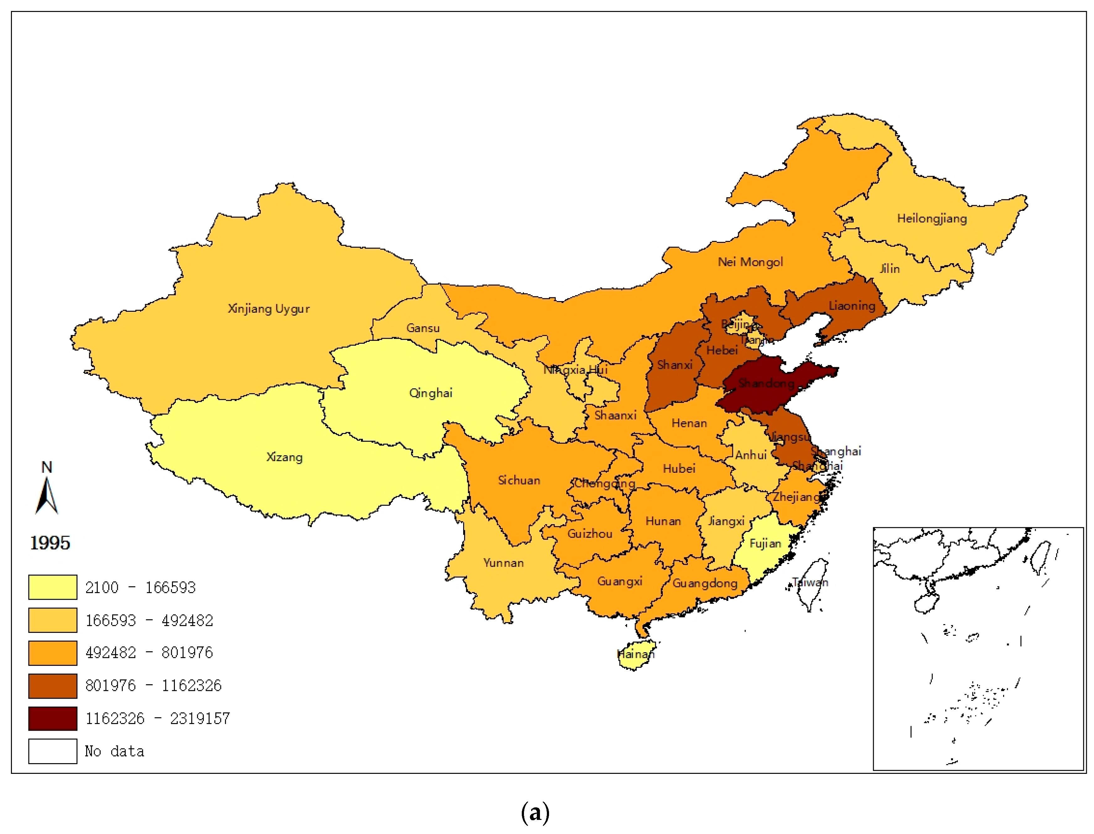
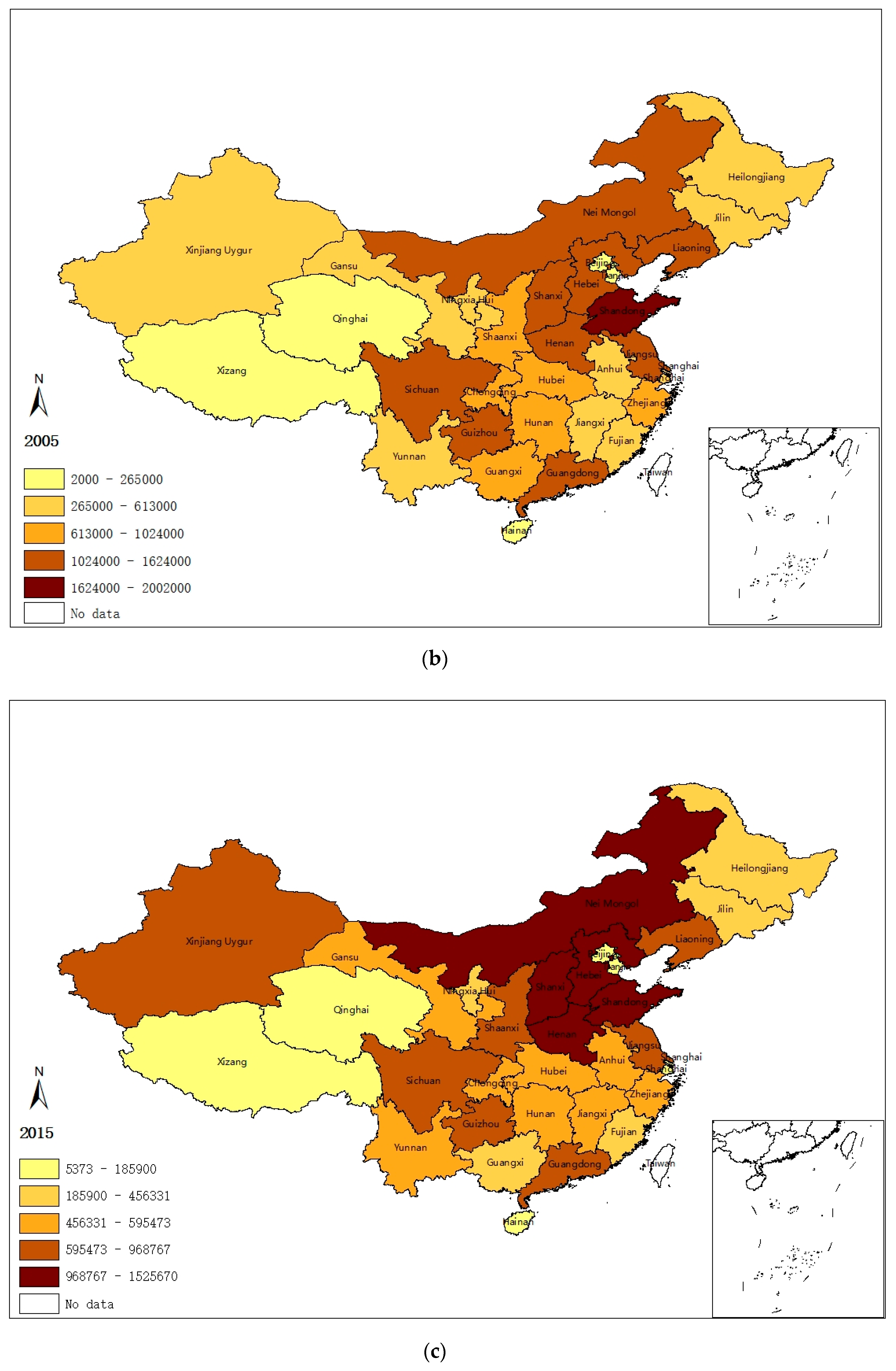
In order to illustrate the geographical distribution of China’s regional sulfur emissions intuitively, natural breaks (Jenks) in ArcGIS are employed to divide the 31 provinces into five categories according to their emissions’ level. Figure 1 illustrates that the spatial distribution of provincial SO2 emissions (1995, 2005, and 2015) is likely to be subject to a certain pattern: (1) a lot of emissions activities cluster in a few provinces; (2) provinces of higher emission level tend to agglomerate together, and so do the provinces with lower emission level; and (3) the western areas tend to be less emission-intensified compared with the northern regions, resulting in a more concentrated and unbalanced spatial pattern of sulfur emissions.
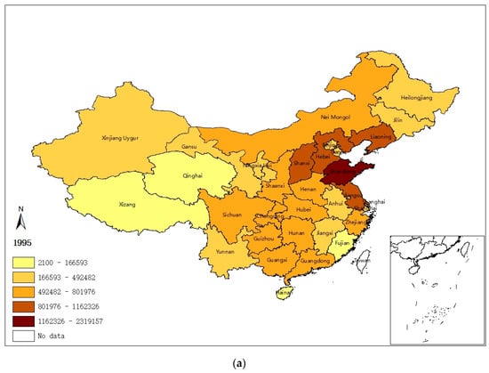
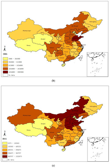
Figure 1.
SO2 emissions in (a) 1995, (b) 2005, and (c) 2015 (Tons).
On the basis of the spatial distributing pattern of SO2 emissions shown by Figure 1, the emissions concentration area can be divided into two parts, namely a north (mainly at/around the Beijing–Tianjin–Hebei region) and a western emission zone. Sulfur emitting activities in the north emission zone are rather more intensive, exhibiting a robust spatiotemporal evolving characteristic over time.
Table 2 illustrates the sulfur emissions’ trend of global spatial autocorrelation during 1995–2015. Most Moran’s I statistics are significant at the 10% level, suggesting the spatial clustering phenomenon of SO2 emissions is not just intuitive, but substantial, and the HH or LL should be the main clustering pattern.
Table 3 lists the SO2 emissions’ time-series correlation. It is clear that the current provincial SO2 emission level highly depends on the levels of prior years. Such time-series dependence only slightly decreases with the increase of the time interval. The space–time evolvement of SO2 emissions and its determinants are worthy of scrutinizing, which will be carried out in the remaining analysis. After observing the SO2 emissions’ geographical evolvement and time–series dependence, the following analysis attempts to unfold the socioeconomic determinants behind the emissions dynamics.

Table 3.
Correlation coefficients of annual SO2 emissions.
3.2. Space–Time Nexus between SO2 Emissions and Its Socioeconomic Determinants
Local spatial patterns’ details can be masked by a bare discussion on global spatial autocorrelation. Besides, economic activities are temporal in essence [56,57], which would significantly affect energy consumption and pollution emissions. In order to cope with the issues, the author adopts the mapping technique of space–time stability, to overlap significant spatial agglomerations (hot and cold spots) on different time points (1995, 2005, and 2015). In this way, the spatiotemporal nexus between SO2 emissions and their socioeconomic factors can be visualized.
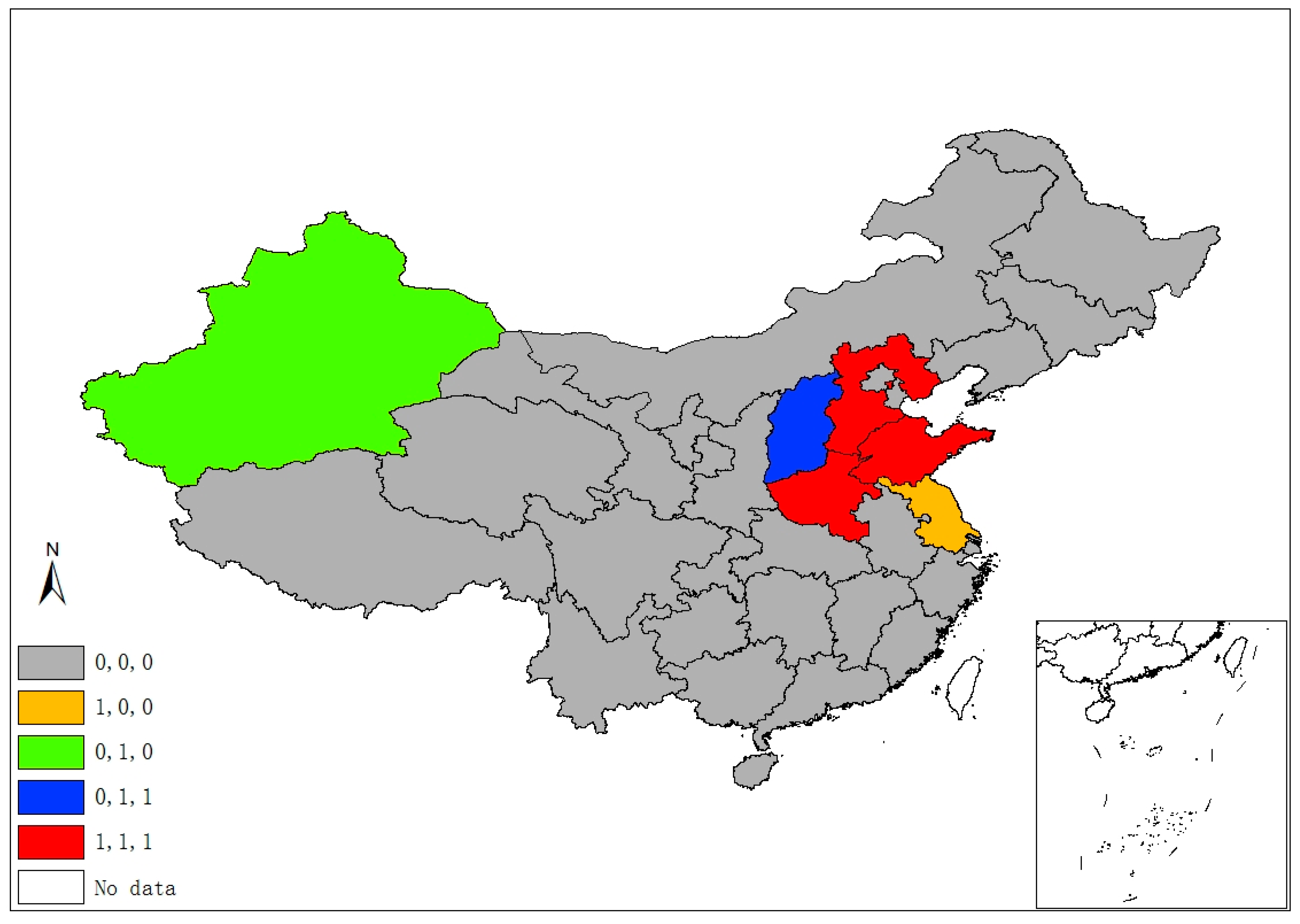
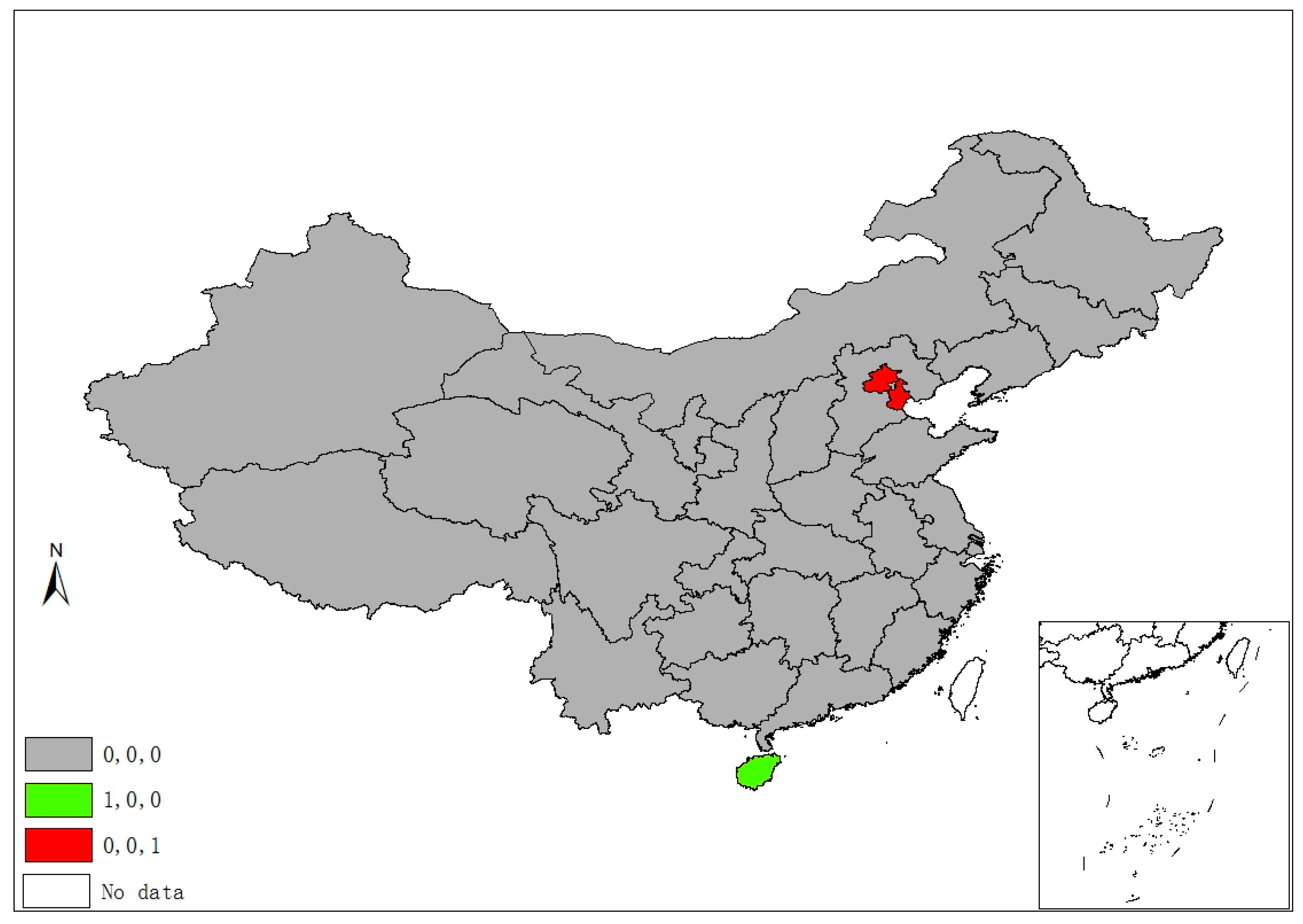
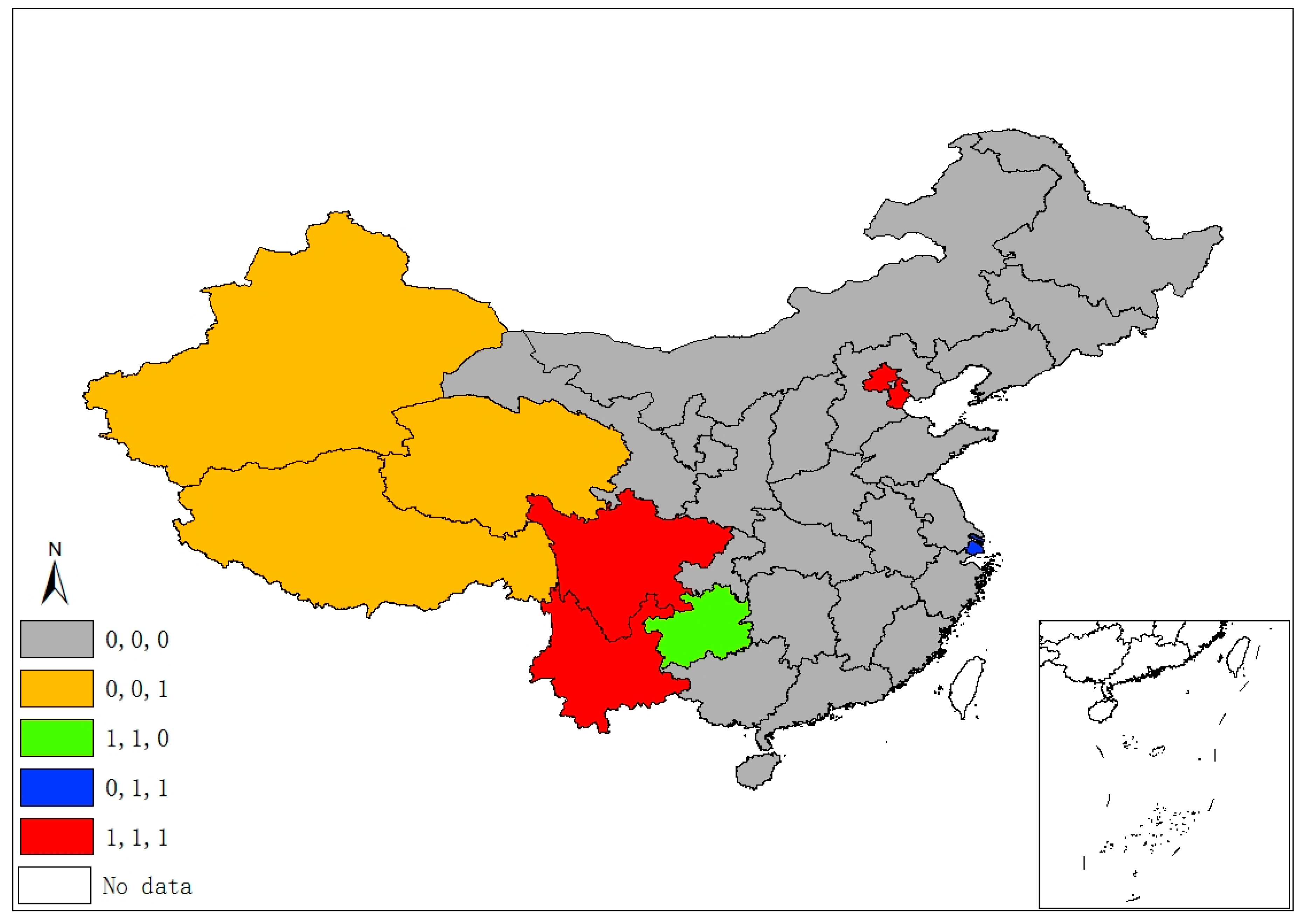
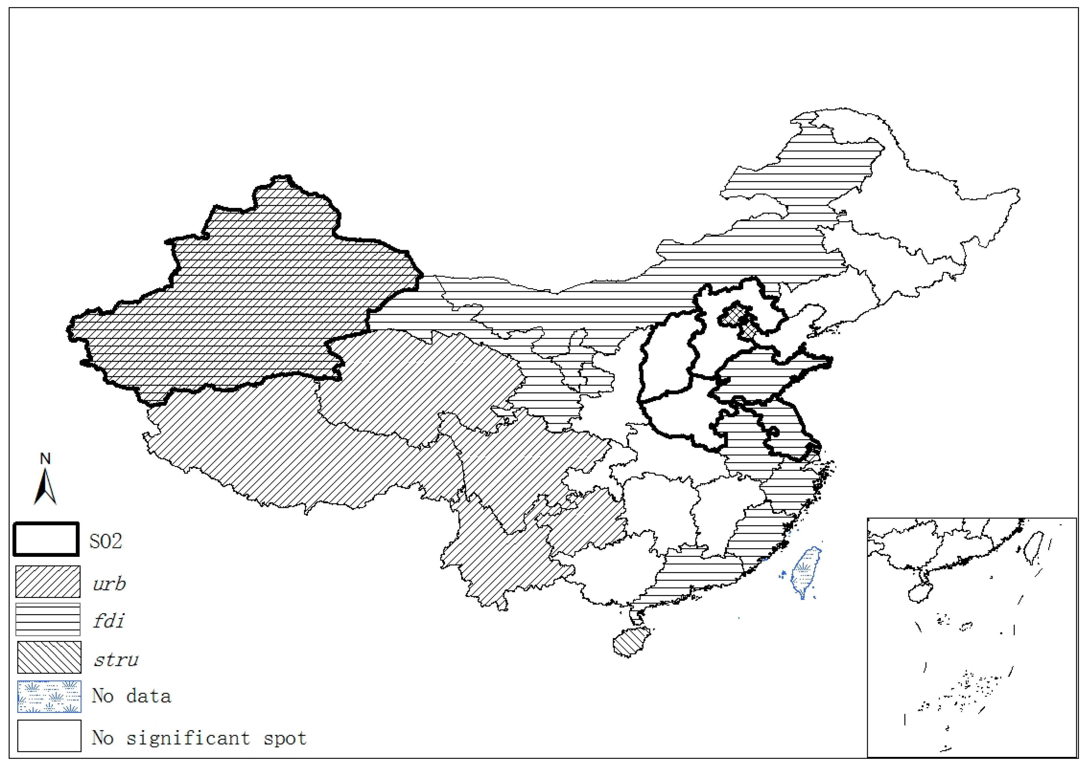
Figure 2 demonstrates five classes of sulfur’s space–time stability. A province is identified as “1, 0, 0”, if it was a significant hot/cold spot in 1995, but not in the latter two years. A province is labeled “0, 1, 0” if it was a significant spot in 2005, but not in 1995 and 2015. Hence, the “0, 1, 1” pattern suggests that a province unit remained a significant spot in latter two years, but not in 1995, and “1, 1, 1” suggests a province was a significant spot in all three years. Finally, if a province had never been a significant spot in any year, it is labeled “0, 0, 0”. Following this manner, Figure 3, Figure 4 and Figure 5 demonstrate different categories of space–time stability of fdi, stru, and urb, respectively.

Figure 2.
Spatiotemporal significant spots of SO2 emissions.
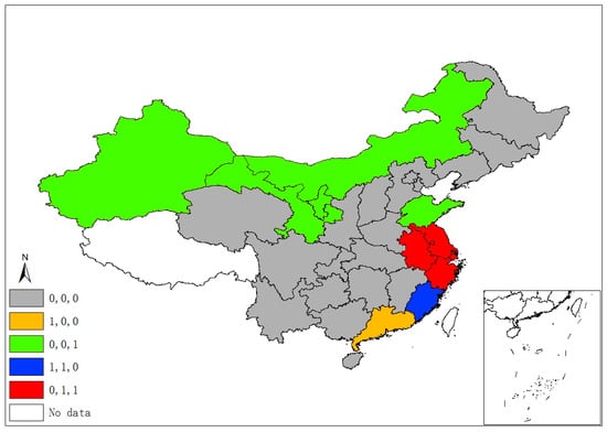
Figure 3.
Spatiotemporal significant spots of foreign direct investment (FDI).

Figure 4.
Spatiotemporal significant spots of industrial structure (stru).
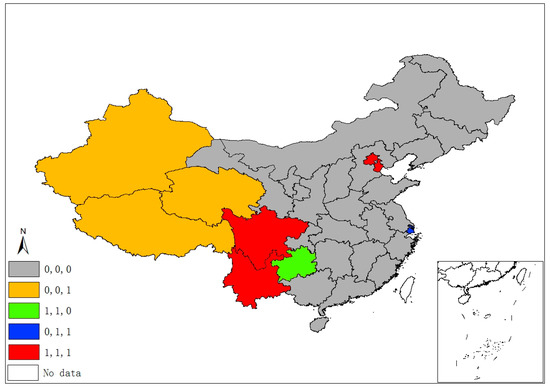
Figure 5.
Spatiotemporal significant spots of urbanization level (urb).
Six provincial units were the SO2 emissions significant hot/cold spots of different four classes, mainly locating at/round the Beijing–Tianjin–Hebei region, which is also the area with more serious air pollution (e.g., smog) in China. Regarding the FDI index, eleven provinces are reported in four categories of significant spots that are mostly located in the north and the eastern coastal economic belt. Significant spots of industrial adjustment index (stru) are identified in three provinces/municipalities (Beijing, Tianjin, and Hainan) with three categories, while significant urbanization spots are identified in the western areas and Beijing, Tianjin, and Shanghai.
The spatiotemporal essences of these four different variables show few similarities, and it is hard to notice any connection between SO2 emissions and the socioeconomic factors in terms of their spatial distribution and temporal evolvement through separate figures (Figure 2, Figure 3, Figure 4 and Figure 5). Thus, Figure 6 overlays significant hot and cold spots of four variables on a single map to demonstrate the comprehensive emissions–determinates nexus in the space–time context. It is noteworthy that the SO2 emissions’ significant spots overlap its three determinant variables and the north and north central regions have more provinces with hot/cold spots over the period. Moreover, Figure 6 also suggests that FDI might have a stronger connection with the spatiotemporal distribution of SO2 emissions in specific areas than urbanization and industrial structure, as SO2 and FDI share more coupled provincial units. Specifically, Xinjiang and its neighbors (Xizang, Qinghai, and Gansu) are all characterized by the low level of emissions, FDI, and urbanization; as such, Xinjiang should form a low–low spatial agglomeration and be a significant cold spot of these three variables. The emission–FDI significant spots can also be found at Shandong and Jiangsu provinces. Beijing is the capital city of China, which has relatively high levels of urbanization and industrial structure development, but is surrounded by Hebei, the emission-intensive and heavily polluted neighbor. Thus, Beijing is identified as the SO2, urb, and stru significant spots.
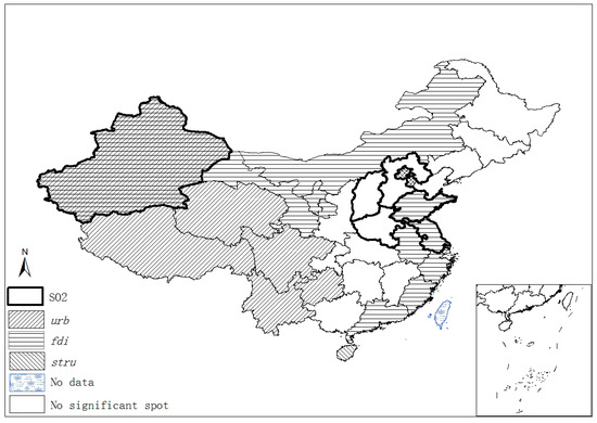
Figure 6.
Comprehensive spatiotemporal significant spots.
The preliminary analysis above indicates that urbanization, FDI, and industrial structure all should have an evidently close connection with sulfur emissions in space–time extent. However, the ESDA technique has limited capability of revealing the causal relationship between the dependent and independent variables, plus it is unable to quantify the determinants’ impacts. Moreover, the data generating process (DGP) is usually unknown in empirical studies. The application of sophisticated statistical inferences and rigorous models can help us to fit the data and better describe the DGP. Therefore, the next subsection further examines the spatiotemporal nexus based on the dynamic SDM introduced in Section 2.3.
3.3. Econometric Results and Interpretation
In the spatial econometric analysis, the negligence of the spatial autocorrelation can lead to biased estimates [52]; in addition, the independent variables’ impacts on dependent variable could be overestimated without the incorporation of the dynamic effects/series dependence [58]. Consequently, it is necessary to control for both time-series dependence and spatial autocorrelation of the dependent variable (lnSO2) within the quantitative empirical framework (dynamic SDM).
Table 4 depicts the coefficients estimated through maximum likelihood estimation [59] of Equations (2)–(4). lnSO2 t − 1, WlnSO2 t − 1, and WlnSO2 t capture the time lag, spatial lag, and space–time lag effects, respectively. Estimations of both γ0 and ρ0 are significant in all three models, suggesting the incorporation of time lag and space–time lag effects is necessary for the empirical framework. Therefore, Equation (2) is superior to Equation (3) and Equation (4), and the following analysis is based on Equation (2). In Equation (2), the λ0 estimation is positive and significant, which means that even with the inclusion of determinants’ spatial lag terms, the model should still control for emissions’ spatial association as well. This validates the Moran’s I statistics results of Table 2. The determinants’ parameters in Table 4 cannot be interpreted as the average response of SO2 emissions to its determinants, because the dynamic SDM includes WlnSO2 t on the right-hand side, and, intrinsically, the partial derivatives of lnSO2 t on the independent variables do not equal to their parameters. Instead, the socioeconomic determinants’ direct and spillover effects need further calculation by plugging the parameters (in Table 4, Equation (2)) into Equations (6) and (7); the results are listed in Table 5.

Table 4.
Coefficients estimates of the dynamic spatial Durbin models.

Table 5.
Short- and long-term effects on SO2 emissions.
Table 5 shows that in China, urbanization, FDI, and industrial structure all have statistically significant influences on SO2 emissions. The formal definition of spillover effects here is the impacts that a specific spatial unit exerts on its adjacent units [55]. In the short run, a 10% increase of FDI level will, ceteris paribus, averagely result in a 0.11% increase of emissions in the adjacent provinces, but would not have any significant influences on the emission level of the local province. In the long run, FDI does not have either direct or spillover effects on SO2 emissions. Urbanization evidently has negative impacts on the local and neighbor sulfur emission levels in the short run, which means the urbanization development can temporarily reduce the SO2 emissions. By contrast, the urbanization rate has no long-term influence on emissions. The industrial adjustment index is negatively related to the local and neighbors SO2 emissions in the short run, while the index is only negatively related to the local emissions in the long run. Besides, population- and energy-related technological advancement (indicated by energy intensity, which is negatively correlated to the technological progress level [21]) also have significant long- and short-term influences on SO2 emissions. A 10% growth of population would, ceteris paribus, averagely lead to a 2.75% and 5.41% temporal increase of emissions in the local and all adjacent provinces, respectively, and eventually, it would lead to a 20.15% increase of local emissions, but no significant change of neighbor emissions. As for the technological progress, its long- and short-term impacts only work on local emissions, but not on emissions of adjacent provinces. All else being equal, a 10% increase of technological progress level will averagely lead to 0.99% and 8.78% decreases of local emissions in the short and long run, respectively.
The dynamic SDM analysis above provides confirmative verification for the findings of ESDA in Section 3.2. China’s SO2 emissions are significantly dependent on FDI, urbanization, and industrial structure in the spatiotemporal context. Moreover, the sulfur emissions’ series dependence could be explained by industrial structure, the population, as well as energy intensity, and these three determinants have profound and eventual impacts on SO2 emissions in China.
4. Discussion
As environmental sustainability and economic development (including urbanization, industrial structure transformation, and international trade) are both critical issues for China’s sustainable development. The focus on emission reduction motivates the discovery of the spatiotemporal characteristics of SO2 emissions. Such explorations could help to develop a scientific foundation for the targeted decomposition of regional emissions, for a better understanding of the mechanisms of cross-region compensation, as well as for region-specific sustainable development. The ESDA results reveal that despite the distinct SO2 emission levels in different years, overall, the clustering pattern had been stable. Similar to the findings in Zhao et al. [35], the emission-intensive provinces mainly agglomerate at/near the Beijing–Tianjin–Hebei region (Figure 1 and Figure 6), which is in correspondence with the serious pollution of fog and haze in this region. Such a high-pollution and emissions phenomenon around the Beijing–Tianjin–Hebei region is closely related to the high proportion of the polluting heavy industry and the relative hysteresis of the tertiary industry development, especially in Hebei province [39]. Shandong and Jiangsu provinces form emission–FDI significant spots owing to their high level of foreign trade openness and emissions. Other than that, the capital city Beijing and municipality Tianjin have high urbanization levels and advanced industrial composition; meanwhile, they are surrounded by many pollution and emission enterprises from near areas. Thus, these two cities are identified as urb– and stru–emission significant spots.
China’s provincial SO2 emissions are found to have significant autocorrelation (Table 2), which is in line with similar previous studies [35,36]. Atmospheric pollutants, especially the emission type, are usually characterized by spatial dependence/diffusions, because adjacent provinces may be the mimics of each other’s socio-economic and environmental policies. Thus, the emissions’ level could be affected by neighbors’ emissions and economic activities including foreign investment promotion, the layout of industrial structure, urban infrastructure, and technological development [5]. China’s central government assigns the annual national achievements of pollution reduction and economic growth at the provincial and prefectural levels. The evaluation of such achievements is carried out among provinces and cities. The competition in economic growth and environmental production inevitably arise between provinces/cities for local governors’ political performance. If a specific local government adopts a strict pollution discharge standard, its neighboring provinces are likely to imitate and implement a similar standard on their own emissions reduction. On the contrary, if the local government takes the development as the primary task and set out a series of loose regulations on pollution emissions, the adjacent provinces are likely to adopt similar loose regulations in order to compete in terms of economic growth. Therefore, such “demonstration effects” should be responsible for the autocorrelation of SO2 emissions found in Section 3 [60].
The dynamic spatial econometric results not only verified, but also quantified the spatiotemporal nexus of the socioeconomic factors to SO2 emissions. The pollution haven hypothesis (PHH) can explain the adverse (positive value) effects of FDI on emissions. The PHH suggests that developed countries’ multinational enterprises, particularly the energy- and pollution-intensive ones, are likely to relocate their business and industries to developing countries owing to the incentives of profits and relatively loose environmental law in these developing countries. Therefore, PHH vividly denotes the less developed countries as a “pollution haven”, if they have lower environmental standards than the necessary level of efficient foreign capital and investment inflow. In this way, such a low barrier of international trade would be environment-deteriorating in China—the provinces with relatively loosen environmental regulations and higher openness of international trade may have been attracting less environment-friendly foreign companies, resulting in considerable pollution emissions [61]. Interestingly, FDI only exerts (short-term) spatial spillover effects on SO2 emissions, but no direct effects. China’s FDI mainly agglomerates at the developed southeast coast economic belt (Figure 6), where stricter regulation, highly advanced-technology, and experienced management exist [35]. Therefore, these areas are able to minimize the FDI’s environmental adverse impact, so that the FDI does not evidently affect the local emissions.
Urbanization’s beneficial effects for the SO2 abatement can be reflected by the modernization theory [62,63]. The urbanization process inevitably consumes more energies and thus generates more pollutants owing to the demand for building materials for constructing new and upgrading old public infrastructures [22]. However, improvements in urbanization level and urban density could also result in an upgrade on the efficiency of public infrastructure’s utilization, such as public transport, which decreases energy consumption and pollution emissions [24,64]. Urbanization also means more advanced and modernized ways of energy consumption. The replacement of inefficient solid fuels by advanced energy utilization enables urban industries and residents to lower the energy consumption and pollution emission levels [65,66]. Moreover, urbanization can promote environmental quality via economies of scale in environmental protection and services of sanitation [67].
The upgrade and optimization (transfer of secondary to tertiary industry) of industrial structure can lead to a reduction of SO2 emissions in local and neighbor provinces of China, because the pollution intensities are distinct in different industries. The secondary industry is the segment of the economy that processes the raw materials (from primary industry) into products and commodities for its consumers, and the secondary industry is also known as the manufacturing industry. The tertiary industry is the economic sector that provides services to the consumers, consisting of a range of businesses, such as entertaining institutions, schools, finance companies, research and development (R&D) departments, and catering services. It is also known as the tertiary/service industry. Given the industries’ production patterns, the secondary industry is more materiel- and energy-consuming, and thus more pollution-intensive. As for the tertiary industry, it is knowledge- and service-intensive, and thus less polluting. Specifically, in China, industrial sectors (mainly in the secondary industry), including the construction sector, are the major source of emissions, accounting for 84% of the total energy-related emissions in 2014 [68]. The industrial sectors’ SO2 emissions make up over 80% of China’s total sulfur emission [69]. On the other hand, the tertiary industry is composed of less-polluting services and light manufacturing sectors. The industrial composition’s effects are long-lasting because the structure varies with economic development all along. At the initial stage, because of the pursuit of industrialization, production resources and capital in primary industry (agricultural sectors) transfer to secondary industry, particularly the heavy industry, which boosts pollution emissions. When it comes to the middle and late stage, the demand of higher efficiency and lower emission causes a shift from the emission-intensive secondary industry towards the knowledge-intensive tertiary industry, so the process reduces the emissions’ amount [20,70]. During 2004–2014, the secondary industry ratio had been decreasing in developed Chinese provinces, and had first increased and then decreased in the developing provinces. China’s recently implemented industrial upgrading reform ought to be responsible for such changes [36].
Technological progress is found to be effective on SO2 abatement in China, which is in line with findings of Zhou et al. [36], Dinda et al. [71], and Ge et al. [26]. According to the facts in China, the reason for the environmental-beneficial effects of technological advancement (a decline of energy intensity) is three-fold: exhaust-gas emission reduction’s upgrade, for example, the end-of-pipe abatement technology; the promotion of energy industrialization; and surging investment in new energy industries [6,72]. REN21 Global Status Report [73] reveals that China has been developing large amounts of new energies that are more sustainable and cleaner, such as hydropower, solar power, biofuels, and wind power. Highly advanced technology tend to be the primary cause that leads to environmental quality improvement in the long term [74]; this can also be seen from the absolute value of lnEI in Table 5. Theoretically, highly advanced technology is usually characterized by efficient utilization of energy and materials during continuous economic growth, which saves more natural resource and reduces the burden on environmental protection of economic activities. The incidentally allowed renewable energies to emerge during technological advancement to enable a country to recycle and reuse the production materials more efficiently, so that they can reserve more natural resources and reduce the emissions [36]. A comparable empirical study also found technological progress to be a major contributor to SO2 abatement in Germany and Netherlands [75].
Different from FDI, technological progress only has direct effects that only influence local SO2 emissions, as geographic boundaries can hinder technology’s spatial-spillovers [76,77]. Without a doubt, public sectors’ R&D activities can transmit through the Internet and multimedia, although the information networks cannot utterly replace the physical communications (e.g., seminars, researcher exchange, field trips, science facilities, and paper documentation). Moreover, monopoly profits are incentives for companies to establish a technological barrier that is effective for removing other competing firms [77], so the technology is found to be non-effective on neighboring provinces’ emissions.
As mentioned above, previous work (Zhou et al. [36], Zhao et al. [35], Zhao et al. [38], Dinda et al. [71], Ge et al. [26], and Rui et al. [39]) also detected significant effects of technology and industrial composition on pollution emissions. However, they ignore these factors’ short-term effects because the application of the traditional static panel model is unable to account for both spatial and series dependence (the DGP’s inherent spatial and temporal characteristics) in the empirical framework, which could lead to biased results [78].
In general, the interprovincial cooperation, imitation, and competition should account for the emissions’ autocorrelation and socioeconomic activities’ spillover effects. Considering China’s continuous industrial structure upgrade and high-speed developing technology, the fundamental driving factors of SO2 emissions’ reduction can be categorized into two types: economic structural and technological progress—a similar opinion can be found in Dinda [19].
5. Conclusions
China’s rapid economic growth is accompanied by soaring energy consumption and pollution emissions; as a result, the country has become one of the largest SO2 emitters in the world. At such a juncture, a clear and precise understanding of the spatiotemporal patterns of China’s SO2 emissions is essential and crucial. Relevant knowledge can constitute a practical framework for policymakers at different administrative levels to achieve the SO2 abatement task and design a mechanism of abatement’s cross-region compensation in China.
The empirical results offer new findings and novel insights into the spatiotemporal dimensions of China’s SO2 emissions and the socioeconomic factors spanning from 1995 to 2015. The main conclusions are summarized as follows.
The ESDA reveals that SO2 emissions and their socioeconomic factors went through a stable and evident spatial clustering pattern during the study period. Spatial externalities of emissions exist across different provincial areas, namely the variation of provincial SO2 emissions influence not only the local provinces, but also the adjacent provinces’ emissions. Several kinds of significant spots are recognized through the mapping technique, suggesting that significant spots of emissions generally overlay well with the influencing factors’ significant spots, and this result reflects the fact that there is a close space–time nexus of SO2 emissions to these factors (FDI, industrial composition, and urbanization).
The econometric empirical analysis is theoretically based on the extended STIRPAT model (Equation (1)) and embeds a dynamics spatial Durbin model to quantify the spatiotemporal nexus in a confirmatory way. Spatial externality plays an important role because the factors’ spillovers significantly contribute to the space- and time-dynamics of China’s SO2 emissions. An increase in population or FDI increases the SO2 emissions. By contrast, the urbanization progress, industrial structure upgrade, and technological advancement can all improve the efficiency of SO2 abatement. The urbanization progress only reduces local and adjacent provinces’ SO2 emissions in the short run, whereas the technological advancement and optimization of industrial composition exert both short- and long-term reducing effects. In other words, the technological advancement and industrial structure update have long-lasting and profound influences on China’s SO2 emissions. Their differences lie in the short-term influence, owing to “demonstration effects”, the industrial composition affects not only local emissions, but also the emissions of neighboring provinces, while the technological progress only influences local emissions owing to geographical barriers.
The study also provides a reference value. China’s policymakers should advocate the optimization of industrial structure and improvement of energy-related technology, which can practically constitute a more thorough and effective way of SO2 abatement. On the other hand, the decision-maker is also urged to curb and then give up the traditional energy- and emission-intensive industries and resource-consuming developing way, and to exchange the immediate interests (e.g., foreign capital inflow with low environmental standards) for securing the long-term sustainable purpose.
As merely 30 Chinese provincial units and 21 years’ time points are analyzed in this paper, owing to the data availability, further studies are expected to adopt less aggregate spatial elements (i.e., prefecture-level, even county-level data) and longer time points to capture more spatial and temporal characteristics. In addition, the issues not covered by this paper, such as the inequality/convergence of SO2 and other pollution emissions, should be addressed from both regional and industry perspectives.
Funding
This research was funded by Lingnan (University) College Fund (0219000088).
Acknowledgments
I would like to thank the anonymous referees for their review, comments, and valuable suggestions.
Conflicts of Interest
The author declares no conflict of interest.
References
- Wang, S.; Fang, C.; Ma, H.; Wang, Y.; Qin, J. Spatial differences and multi-mechanism of carbon footprint based on GWR model in provincial China. J. Geogr. Sci. 2014, 24, 612–630. [Google Scholar] [CrossRef]
- Wang, S.; Fang, C.; Wang, Y.; Huang, Y.; Ma, H. Quantifying the relationship between urban development intensity and carbon dioxide emissions using a panel data analysis. Ecol. Indic. 2015, 49, 121–131. [Google Scholar] [CrossRef]
- Wang, Q.; Zhou, P.; Shen, N.; Wang, S. Measuring carbon dioxide emission performance in Chinese provinces: A parametric approach. Renew. Sustain. Energy Rev. 2013, 21, 324–330. [Google Scholar] [CrossRef]
- Zhao, Y.; Wang, S. The Relationship between Urbanization, Economic Growth and Energy Consumption in China: An Econometric Perspective Analysis. Sustainability 2015, 7, 5609–5627. [Google Scholar] [CrossRef]
- Wang, S.; Zhou, C.; Li, G.; Feng, K. CO2, economic growth, and energy consumption in China’s provinces: Investigating the spatiotemporal and econometric characteristics of China’s CO2 emissions. Ecol. Indic. 2016, 69, 184–195. [Google Scholar] [CrossRef]
- Wang, Y.; Han, R.; Kubota, J. Is there an Environmental Kuznets Curve for SO2 emissions? A semi-parametric panel data analysis for China. Renew. Sustain. Energy Rev. 2016, 54, 1182–1188. [Google Scholar] [CrossRef]
- Boningari, T.; Smirniotis, P.G. Impact of nitrogen oxides on the environment and human health: Mn-based materials for the NOx abatement. Curr. Opin. Chem. Eng. 2016, 13, 133–141. [Google Scholar] [CrossRef]
- Cheng, Z.; Li, L.; Liu, J. Identifying the spatial effects and driving factors of urban PM2.5 pollution in China. Ecol. Indic. 2017, 82, 61–75. [Google Scholar] [CrossRef]
- Schreifels, J.J.; Fu, Y.; Wilson, E.J. Sulfur dioxide control in China: Policy evolution during the 10th and 11th Five-year Plans and lessons for the future. Energy Policy 2012, 48, 779–789. [Google Scholar] [CrossRef]
- Pui, D.Y.; Chen, S.-C.; Zuo, Z. PM 2.5 in China: Measurements, sources, visibility and health effects, and mitigation. Particuology 2014, 13, 1–26. [Google Scholar] [CrossRef]
- Su, S.; Li, B.; Cui, S.; Tao, S. Sulfur Dioxide Emissions from Combustion in China: From 1990 to 2007. Environ. Sci. Technol. 2011, 45, 8403–8410. [Google Scholar] [CrossRef] [PubMed]
- Wei, J.; Guo, X.; Marinova, D.; Fan, J. Industrial SO2 pollution and agricultural losses in China: Evidence from heavy air polluters. J. Clean. Prod. 2014, 64, 404–413. [Google Scholar] [CrossRef]
- Liu, C.; Hong, T.; Li, H.; Wang, L. From club convergence of per capita industrial pollutant emissions to industrial transfer effects: An empirical study across 285 cities in China. Energy Policy 2018, 121, 300–313. [Google Scholar] [CrossRef]
- Xu, Y.; Masui, T. Local air pollutant emission reduction and ancillary carbon benefits of SO2 control policies: Application of AIM/CGE model to China. Eur. J. Oper. Res. 2009, 198, 315–325. [Google Scholar] [CrossRef]
- Cheung, K.-Y.; Lin, P. Spillover effects of FDI on innovation in China: Evidence from the provincial data. China Econ. Rev. 2004, 15, 25–44. [Google Scholar] [CrossRef]
- Wang, H.; Jin, Y. Industrial Ownership and Environmental Performance: Evidence from China; The World Bank: Washington, DC, USA, 2002. [Google Scholar]
- Bao, Q.; Chen, Y.; Song, L. Foreign direct investment and environmental pollution in China: A simultaneous equations estimation. Environ. Dev. Econ. 2011, 16, 71–92. [Google Scholar] [CrossRef]
- Dean, J.M.; Lovely, M.E.; Wang, H. Are Foreign Investors Attracted to Weak Environmental Regulations? Evaluating the Evidence from China; The World Bank: Washington, DC, USA, 2005. [Google Scholar]
- Dinda, S. Environmental Kuznets Curve Hypothesis: A Survey. Ecol. Econ. 2004, 49, 431–455. [Google Scholar] [CrossRef]
- Stern, D.I. The Rise and Fall of the Environmental Kuznets Curve. World Dev. 2004, 32, 1419–1439. [Google Scholar] [CrossRef]
- Zhou, Z. The Underground Economy and Carbon Dioxide (CO2) Emissions in China. Sustainability 2019, 11, 2802. [Google Scholar] [CrossRef]
- Cole, M.A.; Neumayer, E. Examining the Impact of Demographic Factors on Air Pollution. Popul. Environ. 2004, 26, 5–21. [Google Scholar] [CrossRef]
- Parikh, J.; Shukla, V. Urbanization, energy use and greenhouse effects in economic development. Glob. Environ. Chang. 1995, 5, 87–103. [Google Scholar] [CrossRef]
- Chen, H.; Jia, B.; Lau, S. Sustainable urban form for Chinese compact cities: Challenges of a rapid urbanized economy. Habitat Int. 2008, 32, 28–40. [Google Scholar] [CrossRef]
- Yue, W.; Liu, Y.; Fan, P.; Ye, X.; Wu, C. Assessing spatial pattern of urban thermal environment in Shanghai, China. Stoch. Environ. Res. Risk Assess. 2012, 26, 899–911. [Google Scholar] [CrossRef]
- Ge, X.; Zhou, Z.; Zhou, Y.; Ye, X.; Liu, S. A Spatial Panel Data Analysis of Economic Growth, Urbanization, and NOx Emissions in China. Int. J. Environ. Res. Public Heal. 2018, 15, 725. [Google Scholar] [CrossRef] [PubMed]
- Zhou, Y.; Fu, J.; Kong, Y.; Wu, R. How Foreign Direct Investment Influences Carbon Emissions, Based on the Empirical Analysis of Chinese Urban Data. Sustainability 2018, 10, 2163. [Google Scholar] [CrossRef]
- Riti, J.S.; Song, D.; Shu, Y.; Kamah, M. Decoupling CO2 emission and economic growth in China: Is there consistency in estimation results in analyzing environmental Kuznets curve? J. Clean. Prod. 2017, 166, 1448–1461. [Google Scholar] [CrossRef]
- Mahmood, H.; Furqan, M.; Bagais, O. Environmental accounting of financial development and foreign investment: Spatial analyses of East Asia. Sustainability 2019, 11, 13. [Google Scholar] [CrossRef]
- Koçak, E.; Ulucak, Z.S. The effect of energy R&D expenditures on CO2 emission reduction: Estimation of the STIRPAT model for OECD countries. Environ. Sci. Pollut. Res. 2019, 26, 14328–14338. [Google Scholar]
- Gong, X.; Mi, J.; Yang, R.; Sun, R. Chinese National Air Protection Policy Development: A Policy Network Theory Analysis. Int. J. Environ. Res. Public Heal. 2018, 15, 2257. [Google Scholar] [CrossRef]
- Gong, X.; Mi, J.; Wei, C.; Yang, R. Measuring Environmental and Economic Performance of Air Pollution Control for Province-Level Areas in China. Int. J. Environ. Res. Public Heal. 2019, 16, 1378. [Google Scholar] [CrossRef]
- Ding, Y.; Zhang, M.; Chen, S.; Wang, W.; Nie, R. The environmental Kuznets curve for PM2.5 pollution in Beijing-Tianjin-Hebei region of China: A spatial panel data approach. J. Clean. Prod. 2019, 220, 984–994. [Google Scholar] [CrossRef]
- Chen, X.; Yi, G.; Liu, J.; Liu, X.; Chen, Y. Evaluating Economic Growth, Industrial Structure, and Water Quality of the Xiangjiang River Basin in China Based on a Spatial Econometric Approach. Int. J. Environ. Res. Public Heal. 2018, 15, 2095. [Google Scholar] [CrossRef] [PubMed]
- Zhao, X.; Deng, C.; Huang, X.; Kwan, M.-P. Driving forces and the spatial patterns of industrial sulfur dioxide discharge in China. Sci. Total. Environ. 2017, 577, 279–288. [Google Scholar] [CrossRef] [PubMed]
- Zhou, Z.; Ye, X.; Ge, X. The Impacts of Technical Progress on Sulfur Dioxide Kuznets Curve in China: A Spatial Panel Data Approach. Sustainability 2017, 9, 674. [Google Scholar] [CrossRef]
- Yang, X.; Wang, S.; Zhang, W.; Zhan, D.; Li, J. The impact of anthropogenic emissions and meteorological conditions on the spatial variation of ambient SO2 concentrations: A panel study of 113 Chinese cities. Sci. Total. Environ. 2017, 584, 318–328. [Google Scholar] [CrossRef] [PubMed]
- Zhao, H.; Guo, S.; Zhao, H. Impacts of GDP, Fossil Fuel Energy Consumption, Energy Consumption Intensity, and Economic Structure on SO2 Emissions: A Multi-Variate Panel Data Model Analysis on Selected Chinese Provinces. Sustainability 2018, 10, 657. [Google Scholar] [CrossRef]
- Li, R.; Fu, H.; Cui, L.; Li, J.; Wu, Y.; Meng, Y.; Wang, Y.; Chen, J. The spatiotemporal variation and key factors of SO2 in 336 cities across China. J. Clean. Prod. 2019, 210, 602–611. [Google Scholar] [CrossRef]
- Giacomini, R.; Granger, C.W. Aggregation of space-time processes. J. Econ. 2004, 118, 7–26. [Google Scholar] [CrossRef]
- Anselin, L. Spatial Effects in Econometric Practice in Environmental and Resource Economics. Am. J. Agric. Econ. 2001, 83, 705–710. [Google Scholar] [CrossRef]
- Belotti, F.; Hughes, G.; Mortari, A.P. Spatial Panel-data Models Using Stata. Stata J. Promot. Commun. Stat. Stata 2017, 17, 139–180. [Google Scholar] [CrossRef]
- Grossman, G.M.; Krueger, A.B. Economic Growth and the Environment. Q. J. Econ. 1995, 110, 353–377. [Google Scholar] [CrossRef]
- Martínez-Zarzoso, I.; Bengochea-Morancho, A.; Morales-Lage, R. The impact of population on CO2 emissions: Evidence from European countries. Environ. Resour. Econ. 2007, 38, 497–512. [Google Scholar] [CrossRef]
- York, R.; Rosa, E.A.; Dietz, T. STIRPAT, IPAT and ImPACT: Analytic tools for unpacking the driving forces of environmental impacts. Ecol. Econ. 2003, 46, 351–365. [Google Scholar] [CrossRef]
- Anselin, L.; Syabri, I.; Kho, Y. GeoDa: An Introduction to Spatial Data Analysis. Geogr. Anal. 2006, 38, 5–22. [Google Scholar] [CrossRef]
- Yu, D.; Wei, Y.D. Spatial data analysis of regional development in Greater Beijing, China, in a GIS environment. Pap. Reg. Sci. 2008, 87, 97–117. [Google Scholar] [CrossRef]
- Moran, P.A.P. Notes on Continuous Stochastic Phenomena. Biometrika 1950, 37, 17–23. [Google Scholar] [CrossRef]
- Ord, J.K.; Getis, A. Testing for Local Spatial Autocorrelation in the Presence of Global Autocorrelation. J. Reg. Sci. 2001, 41, 411–432. [Google Scholar] [CrossRef]
- Getis, A.; Ord, J.K. The Analysis of Spatial Association by Use of Distance Statistics. Geogr. Anal. 2010, 24, 189–206. [Google Scholar] [CrossRef]
- Ye, X.; Wu, L. Analyzing the dynamics of homicide patterns in Chicago: ESDA and spatial panel approaches. Appl. Geogr. 2011, 31, 800–807. [Google Scholar] [CrossRef]
- Elhorst, J.P. Spatial Econometrics from Cross-Sectional Data to Spatial Panels; Springer: Heidelberg, Germany, 2014. [Google Scholar] [CrossRef]
- Vega, S.H.; Elhorst, J.P. The slx model. J. Reg. Sci. 2015, 55, 339–363. [Google Scholar] [CrossRef]
- Baltagi, B. Econometric Analysis of Panel Data; John Wiley & Sons: Hoboken, NJ, USA, 2008. [Google Scholar]
- Lesage, J.; Pace, R.K. Introduction to Spatial Econometrics; Informa UK Limited; Chapman and Hall/CRC: Boca Raton, FL, USA, 2009. [Google Scholar]
- Rey, S.J.; Ye, X. Comparative spatial dynamics of regional systems. In Progress in Spatial Analysis; Springer: Berlin, Germany, 2010; pp. 441–463. [Google Scholar]
- Ye, X.; Rey, S. A framework for exploratory space-time analysis of economic data. Ann. Reg. Sci. 2013, 50, 315–339. [Google Scholar] [CrossRef]
- Sheng, P.; Guo, X. The Long-run and Short-run Impacts of Urbanization on Carbon Dioxide Emissions. Econ. Model. 2016, 53, 208–215. [Google Scholar] [CrossRef]
- Yu, J.; De Jong, R.; Lee, L.-F. Estimation for spatial dynamic panel data with fixed effects: The case of spatial cointegration. J. Econ. 2012, 167, 16–37. [Google Scholar] [CrossRef]
- Li, Q.; Song, J.; Wang, E.; Hu, H.; Zhang, J.; Wang, Y. Economic growth and pollutant emissions in China: A spatial econometric analysis. Stoch. Environ. Res. Risk Assess. 2013, 28, 429–442. [Google Scholar] [CrossRef]
- Cole, M.A. Trade, the pollution haven hypothesis and the environmental Kuznets curve: Examining the linkages. Ecol. Econ. 2004, 48, 71–81. [Google Scholar] [CrossRef]
- Ehrhardt-Martinez, K. Social Determinants of Deforestation in Developing Countries: A Cross-National Study. Soc. Forces 1998, 77, 567–586. [Google Scholar] [CrossRef]
- Martinez-Zarzoso, I.; Maruotti, A. The impact of urbanization on CO2 emissions: Evidence from developing countries. Ecol. Econ. 2011, 70, 1344–1353. [Google Scholar] [CrossRef]
- Liddle, B. Demographic Dynamics and Per Capita Environmental Impact: Using Panel Regressions and Household Decompositions to Examine Population and Transport. Popul. Environ. 2003, 26, 23–39. [Google Scholar] [CrossRef]
- Pachauri, S. An analysis of cross-sectional variations in total household energy requirements in India using micro survey data. Energy Policy 2004, 32, 1723–1735. [Google Scholar] [CrossRef]
- Pachauri, S.; Jiang, L. The household energy transition in India and China. Energy Policy 2008, 36, 4022–4035. [Google Scholar] [CrossRef]
- Torras, M.; Boyce, J.K. Income, inequality, and pollution: A reassessment of the environmental Kuznets Curve. Ecol. Econ. 1998, 25, 147–160. [Google Scholar] [CrossRef]
- Yu, S.; Hu, X.; Fan, J.-L.; Cheng, J. Convergence of carbon emissions intensity across Chinese industrial sectors. J. Clean. Prod. 2018, 194, 179–192. [Google Scholar] [CrossRef]
- Ministry of Ecology and Environment (MEE). Bulletin of National Environmental Statistics (2015); Ministry of Ecology and Environment of the People’s Republic of China: Beijing, China, 2017.
- Suri, V.; Chapman, D. Economic growth, trade and energy: Implications for the environmental Kuznets curve. Ecol. Econ. 1998, 25, 195–208. [Google Scholar] [CrossRef]
- Dinda, S.; Coondoo, D.; Pal, M. Air quality and economic growth: An empirical study. Ecol. Econ. 2000, 34, 409–423. [Google Scholar] [CrossRef]
- Zhang, C.; Lin, Y. Panel estimation for urbanization, energy consumption and CO2 emissions: A regional analysis in China. Energy Policy 2012, 49, 488–498. [Google Scholar] [CrossRef]
- REN21, P.S. Renewables 2014: Global Status Report; REN21 Secretariat: Paris, France, 2014. [Google Scholar]
- Galeotti, M.; Lanza, A. Richer and cleaner? A study on carbon dioxide emissions in developing countries. Energy Policy 1999, 27, 565–573. [Google Scholar] [CrossRef]
- Bruyn, D.S.M. Explaining the Kuznets curve. Structural change and international agreements in reducing sulphur emissions. Environ. Dev. Econ. 1997, 2, 485–502. [Google Scholar] [CrossRef]
- Krugman, P. Increasing Returns and Economic Geography. J. Politi. Econ. 1991, 99, 483–499. [Google Scholar] [CrossRef]
- Miao, F.U. Geographical Distance and Technological Spillover Effects: A Spatial Econometric Explanation of Technological and Economic Agglomeration Phenomena. China Econ. Q. 2009, 8, 1549–1566. [Google Scholar]
- Pirotte, A.; Mur, J. Neglected dynamics and spatial dependence on panel data: Consequences for convergence of the usual static model estimators. Spat. Econ. Anal. 2017, 12, 202–229. [Google Scholar] [CrossRef]
© 2019 by the author. Licensee MDPI, Basel, Switzerland. This article is an open access article distributed under the terms and conditions of the Creative Commons Attribution (CC BY) license (http://creativecommons.org/licenses/by/4.0/).

