Article

Statistical Characteristics of Major Sudden Stratospheric Warming Events in CESM1-WACCM: A Comparison with the JRA55 and NCEP/NCAR Reanalyses

1
Key Laboratory of Meteorological Disaster, Ministry of Education (KLME)/Joint International Research Laboratory of Climate and Environment Change (ILCEC)/Collaborative Innovation Center on Forecast and Evaluation of Meteorological Disasters (CIC-FEMD), Nanjing University of Information Science & Technology, Nanjing 210044, China
2
Fredy & Nadine Herrmann Institute of Earth Sciences, The Hebrew University of Jerusalem, Edmond J. Safra Campus, Givat Ram, Jerusalem 91904, Israel
*
Author to whom correspondence should be addressed.
Atmosphere 2019, 10(9), 519; https://doi.org/10.3390/atmos10090519
Submission received: 25 July 2019 / Revised: 17 August 2019 / Accepted: 2 September 2019 / Published: 4 September 2019
(This article belongs to the Section Meteorology)

Abstract

:
Using the historical simulation from the CESM1-WACCM coupled model and based on the JRA55 and NCEP/NCAR reanalyses, the general statistical characteristics of the major sudden stratospheric warmings (SSWs) in this stratosphere-resolving model are assessed. The statistical and diagnostic results show that CESM1-WACCM can successfully reproduce the frequency of SSW events. As in the JRA55 and NCEP/NCAR reanalyses, five or six SSW events, on average, occur in a model decade. The seasonal distribution of SSWs is also well simulated with the highest frequency in January (35%). The unprecedented low SSW frequency observed in 1990s from the two reanalyses is also identified in a model decade (1930s). In addition, the overestimated duration of SSW events in the earlier WACCM version is not identified in CESM1-WACCM when compared with the two reanalyses. The model can well reproduce the downward propagation of the stratospheric anomaly signals (i.e., zonal wind, height, temperature) following SSWs. Both the modelling and observational evidences indicate that SSWs are proceeded by the positive Pacific–North America (PNA) and negative Western Pacific (WP) pattern. The negative North Atlantic Oscillation (NAO) develops throughout the SSW life cycle, which is successfully modeled. A cold Eurasian continent–warm North American continent pattern is observed before SSWs at 850 h Pa, while the two continents are anomalously cold after SSWs in both the reanalyses and the model.

1. Introduction

Major sudden stratospheric warming (SSW) is a radical and rapid warming phenomenon mainly observed in the Arctic stratosphere during wintertime except the September 2002 SSW over Antarctic [1,2]. When SSW events occur, the polar cap temperature suddenly rises and increases by tens of Kelvins within several days. In the meantime, the stratospheric circulation also adjusts: westerlies in the circumpolar region considerably decrease and even reverse the sign to easterlies; the stratospheric cyclone in the high latitudes gradually shifts from the polar region, deforms in its shape, and even breaks up into two sister vortices [3,4]. Since this phenomenon was first detected by Richard Scherhag [5], much work has been done about SSWs, including their theories [6,7,8], classifications [9], effects on surface weather and climate [10,11,12], simulations in models [13,14,15], and predictions [16,17].
As various observational techniques have been used to detect the stratosphere [18], and various aspects of SSW events (e.g., dynamics, impacts, modelling, and predictions) are explored in literature [8,12,13,15], the understanding about SSW events has been improving gradually. It has been reported that SSW events have a close relationship with planetary wave activity originating from the extratropical troposphere [6,9,15,19,20]. For instance, vortex-displacement SSW events are related to the anomalous amplification of wavenumber-1 planetary waves while vortex-splitting SSW events are caused by the anomalous amplification of wavenumber-two planetary waves [6,19,21]. Additionally, many studies have shown that the occurrence of SSW events can be controlled by some external factors, such as the 11-yr solar cycle [22], the Quasi-Biennial Oscillation (QBO) [23,24,25], El Niño-Southern Oscillation [26], Madden–Julian Oscillation [15,27,28], and stratospheric zonal ozone anomalies [29].
The stratosphere also has significant effect on the troposphere since the anomalous signals in the stratosphere related to SSWs can propagate downward [30,31,32,33]. Therefore, SSWs have significant and deep implications in predicting the weather conditions and climate anomalies in the troposphere [34], due to the feature of the zonal mean signals propagating downward from the stratosphere to the troposphere [30,31]. In specific, following SSW events, the Arctic Oscillation (AO) and Northern Annular Mode (NAM) indices tend to become negative, along with pressure/height rising in circumpolar latitudes and dropping in middle latitudes, while a strong polar vortex usually corresponds to positive AO/NAM [2]. Since a good understanding of dramatic stratospheric circulation variations, especially SSW events, is helpful for improving weather forecasts and climate prediction, much effort has been put into developing stratosphere-resolving models [35].
Not only has modelling SSW events and their impacts on troposphere and surface attracted great attention [36], the predictability of SSW events in the forecast system models has also been evaluated in the most recent studies through analyzing specific cases and using different models [13,17,37,38,39,40]. The predictability of SSW events has been reviewed in Tripathi et al. [36], ranging from several days to near a month depending on different case studies. Many studies have considered the predictability of single SSW cases based on particular models (e.g., four SSWs/the European Centre For Medium Range Weather Forecasts model (ECMWF) in Simmons et al. [41]; December 2001/the Japan Meteorological Agency model (JMA) in Mukougawa et al. [16]; January 2004/JMA in Hirooka et al. [42]; January 2009/the Navy Operational Global Atmospheric Prediction System (NOGAPS) in Kim and Flatau [13]; January 2010/ECMWF in Dörnbrack et al. [14]; February 2018/the China Meteorological Administration Beijing Climate Center model (CMA-BCC) in Rao et al. [15]).
It is noticed that few studies systematically evaluate the reproducibility of SSWs over a long period from a statistical and dynamical perspective. As one of the state-of-the-art stratosphere-resolving models, the Community Earth System Model version 1—the Whole Atmosphere Community Climate Model (CESM1-WACCM), which is one of the models participating in the Coupled Model Intercomparison Project Phase 5 (CMIP5), shows a good stratospheric behavior on the interannual timescale [26,43]. However, statistical characteristics of SSW events in CESM1-WACCM also deserve further exploring. Therefore, we will seek to answer the following two questions in this paper: (1) How well does CESM1-WACCM simulate the radical stratospheric phenomenon, the SSW events? (2) How similar is the evolution of tropospheric circulation during SSW events in CESM1-WACCM and the reanalyses? Evaluating and examining CESM1-WACCM in reproducing SSW events can help model developers better locate the model bias and further improve the model performance. In addition, evaluating CESM1-WACCM is also a necessary step to understand the improvement in CESM2-WACCM in simulating SSW events, which might be reported in the future study.
The structure of the paper is organized as follows. Following the introduction in this section, Section 2 introduces the reanalyses and model datasets, and methods of identifying SSW onset dates and of calculating teleconnections. In Section 3, a parallel comparison of major SSWs between the reanalyses and the model is performed in different aspects, including statistics, stratospheric and tropospheric circulation evolutions, upward planetary waves for major SSWs, and their downward impacts. In Section 4, we present the summary and discussion.

2. Data and Methods

2.1. Reanalyses and Model Data

The historical-run outputs used in this study were integrated by the CESM1-WACCM model [44], one of the fully coupled CMIP5 models. The historical run started from 1850 (model time) and ended in 2005 (model time) and produced a 156-yr dataset. The variables used in the study include air temperature, zonal and meridional winds, and geopotential height. The raw outputs are stored in the model resolution with 66 sigma/pressure levels from 1000 h Pa to 5.1 × 10⁻⁶ h Pa (approximately 140 km) and a horizontal resolution of 1.9° (latitude) × 2.5° (longitude). Specifically, the WACCM model has 18 pressure levels between the surface and 100 h Pa, and 17 levels between 100 h Pa and 3.54 h Pa (approximately 40 km). The atmospheric component of CESM1-WACCM, WACCM4 is a superset of the Community Atmospheric Model version 4 [45,46]. Significant advances in WACCM4 include parameterization of non-orographic gravity waves generated by frontal systems and convection, and especially the addition of a parameterization to estimate mountain stress caused by unresolved orography [47], which has led to a considerable perfection in the simulation of the frequency of northern winter sudden stratospheric warming events by changing the propagation of planetary waves into the polar vortex [45]. The model includes a prescribed representation of the quasi-biennial oscillation (QBO), achieved by relaxing equatorial zonal winds between 86 and 4 h Pa to observed interannual variability (i.e., the idealized 28-month QBO cycle of tropical zonal winds). The prescribed QBO phase varies in time with an approximate 28-month period [45,46,47]. The CESM1-WACCM model also includes interactive chemistry module to produce ozone [45].
In order to evaluate the CESM1-WACCM performance in modelling SSWs, a comparison is made with two reanalyses as an alternative representation of the actual condition of atmosphere in observations. One dataset is the National Centers for Environmental Prediction—National Center for Atmospheric Research Reanalysis I (NCEP/NCAR) dataset. The reference state is extracted from the NCEP/NCAR reanalysis, spanning from 1948–2015 [48]. The daily mean variables used in the study include the air temperature, zonal and meridional winds, and geopotential height. The horizontal resolution of the NCEP/NCAR dataset is 2.5° (latitude) × 2.5° (longitude) and there are 17 pressure levels in the vertical direction extending from 1000 h Pa to 10 h Pa.
The other dataset is the Japanese Meteorological Agency 55-year Reanalysis (JRA55) as an alternative reference [49]. Considering the SSW sample size is limited and large uncertainty is still present in the NCEP/NCAR reanalysis, the JRA55 has been widely used to study the stratospheric variability, such as the momentum budget, the stratospheric annular mode, the Brewer-Dobson circulation, and the stratospheric El Niño–Southern Oscillation (ENSO) teleconnection [46,50,51,52]. Due to some possible uncertainties of using only one reanalysis [50,51], both the NCEP/NCAR and JRA55 reanalyses are shown with caution in this paper. It has been shown that the JRA55 reanalysis can well quantify the annular modes and the ENSO pathway in the stratosphere [46,50]. The JRA55 reanalysis has a horizontal resolution of 1.25° (latitude) × 1.25° (longitude) and 37 pressure levels with the top level at 0.1 h Pa [49].

2.2. Methods

Generally, the identification of a major SSW has been based on one of the WMO definitions [8,9,53]: the day when the zonal mean zonal wind at 60° N and 10 h Pa turns from westerly winds to easterly winds and lasts for more than five days afterwards, is defined here as the zeroth day (day 0) of a sudden warming event and it has been observed mostly in the Northern Hemisphere. In the meantime, the zonal mean temperature in polar cap area increases and the meridional temperature gradients from 60° N to the North Pole at 10 h Pa reverse direction. If the temperature gradient reverses while the circulation does not, it is defined to be a minor SSW, which occur in both hemispheres. Provided that the average length of an SSW event is limited and there will be repetition of zonal wind reversal between westerlies and easterlies, no new SSW events will be defined again within 20 consecutive days after a former SSW event is identified already [8,9]. In addition, stratospheric final warming is excluded as the zonal mean zonal winds change from westerlies to easterlies and stay unchanged in the direction since it marks the annual cycle of the stratospheric circulation from wintertime to summertime [54].
It has been reported that the stratospheric polar vortex intensity and polar cap temperature are closely correlated with the upward propagation of planetary waves from the troposphere to stratosphere [15,20,46]. Furthermore, existing studies also indicate that SSW events might be triggered by the intensification of positive Pacific–North America (PNA) [20,55] and the negative western Pacific (WP) oscillation [56,57]. Additionally, large circulation anomalies in the stratosphere are related to changes in the North Atlantic Oscillation (NAO) [20,52,58]. In order to compare the simulation performance for SSWs, three teleconnection indices are calculated and their definitions [59] are as follows:
WP = 1 2 ( Z 60 ° N ,   155 ° E Z 30 ° N ,   155 ° E )
PNA = 1 4 ( Z 20 ° N ,   160 ° W Z 45 ° N ,   165 ° W + Z 55 ° N ,   115 ° W Z 30 ° N ,   85 ° W )
NAO = 1 2 ( Z 35 ° N ,   0 ° E Z 65 ° N ,   20 ° W )
where Z is the geopotential height anomaly at 500 h Pa and the subscript is the latitude ( ° N ) and longitude ( ° W , ° E ) of the targeted grids on Earth. The anomaly here refers to the deviation of raw daily data from their daily climatology over 1958–2015/1948–2015 (1850–2005) for the JRA55 and NCEP/NCAR reanalysis (CESM1-WACCM run). In addition, the Student’s t-test is used to test the significance level of the composite for one sample ensemble (degree of freedom, or dof = sample size minus one) or the model minus the reanalysis difference (dof = sum of the two sample sizes minus two). We have hypothesized that SSWs are independent events. Because the circulation for one SSW event is persistent, the effective dof for the 10-day mean composite is much less than 10 × the sample size, for example. We still use the original dof based on the sample size for strictness and simplicity by regarding the 10-day mean of every SSW as an independent sample.

3. Parallel Comparison of SSWs between the Reanalyses and CESM1-WACCM

3.1. Statistics of SSW Events

Based on the WMO definition, the onset dates of SSW events in the JRA55 reanalysis during 1958–2015 the NCEP/NCAR reanalysis during 1948–2015, and in the CESM1-WACCM historical run during 1850–2005 were searched and listed in Table 1.
The SSW onset dates in this study are also compared with previous studies [9,20,53,60,61,62], and they are generally consistent. There are 35 SSW events in the JRA55 reanalysis and 38 SSW events in the NCEP/NCAR reanalysis, so the average frequency is 5–6× per decade. However, the SSW events in both reanalyses are not evenly distributed in years. In specific, an inter-decadal variation in SSW occurrence is noticed, although this finding might be sensitive to the SSW definition [53]. Some SSWs are concentrated within a decade while others are more scattered. For example, ten SSW events happened in nine years from 1965 to 1973 while no SSW events occurred during 1990–1997 in the reanalyses. Generally, SSW can happen from November to March. Several years even witnessed two SSW events in one winter: 1965/66, 1968/69, 1969/70, 1970/71, 1987/88, 1998/99, 2007/08, 2009/10. The major SSW events in the reanalyses were generally consistent, but some differences are also noticed in several winters, especially before 1979.
The identical SSW definition is used to search the SSW onset dates in CESM1-WACCM (Table 1). There are 80 SSW events during 1850–2005, so the average frequency is 5 × per decade, similar to that in the reanalyses. The SSW occurrence dates and years are also irregularly distributed in the model. Namely, no SSW events happened during 1881–1886 and eight SSW events appear from 1985–1995. The SSW onset dates in the model are all different from the reanalyses, because the model data used here are from an atmosphere-ocean coupled historical run. The similar SSW occurrence dates for the January 1958, March 1965, January 1977, February 1981, and February 1989 events are simply a coincidence in CESM1-WACCM and the reanalyses.
The seasonal distribution of SSW events is shown in Figure 1 for the reanalyses and the model, respectively. SSW events only happen in wintertime months, from November to March. Some tiny differences in the frequency of SSW onset are noticed between the model and the reanalyses in Figure 1. The January SSWs from both the reanalyses and the model rank the first in their frequency, as almost 35% of the SSW events in the reanalyses and the model appear in January. The February SSWs rank the second in their percentage among the five months in both the model and reanalyses, followed by the March and December SSW events. In contrast, fewest SSW events happen in November. However, there are also some minor differences between the two reanalyses. For example, SSW events in the JRA55 happen more frequently in January than in the NCEP/NCAR, while the situation is reversed in November and March. It seems that the month-to-month contrast in the SSW frequency might be weaker in the NCEP/NCAR than the JRA55. The SSW frequency from the model resembles that in the JRA55 in early winter (November, December) while it is similar to the NCEP/NCAR in January and March by visual inspection. In summary, the frequency distribution in the model is well simulated for the peak in January and the minimum in November.
The decadal distribution of the occurrence number of SSW events is shown in Figure 2 for the JRA55, NCEP/NCAR and CESM1-WACCM, respectively. Out of the last seven decades, 1990s witnessed the fewest SSW events in reanalyses while much more SSW events happen in 2000s. It can be found that, since 1950s, there is a slight rising tendency in the number of SSW occurrence every decade followed by a sharp drop in 1990s and an abrupt increase in 2000s in both reanalyses. Similarly, the model also shows very few SSWs in a model decade (1930s), which might reflect the internal variability of the stratosphere, similar to the real 1990s in the reanalyses. However, the occurrence number of SSW events is quite uniform from 1850s (model decade) to 1910s in the model. In general, the average occurrence number maintains around five times per decade.
According to previous studies [9,43], the amplitude of SSWs can be measured by the area-weighted mean polar cap temperature anomalies in the stratosphere around the SSW onset date. The composite SSW amplitude in each winter month is shown in Figure 3. The composite SSW amplitude in December and January is relatively stronger than in other wintertime months for the reanalyses, and the composite amplitude of SSWs in March is almost half of that in November. The SSW amplitude, especially in midwinter (December, January, February), is realistically reproduced by the model: the composite temperature anomalies fall between the two reanalyses. However, the simulated SSW amplitude in November and March is somewhat overestimated, and the composite SSW amplitude in March from the model is nearly twice that from JRA55.

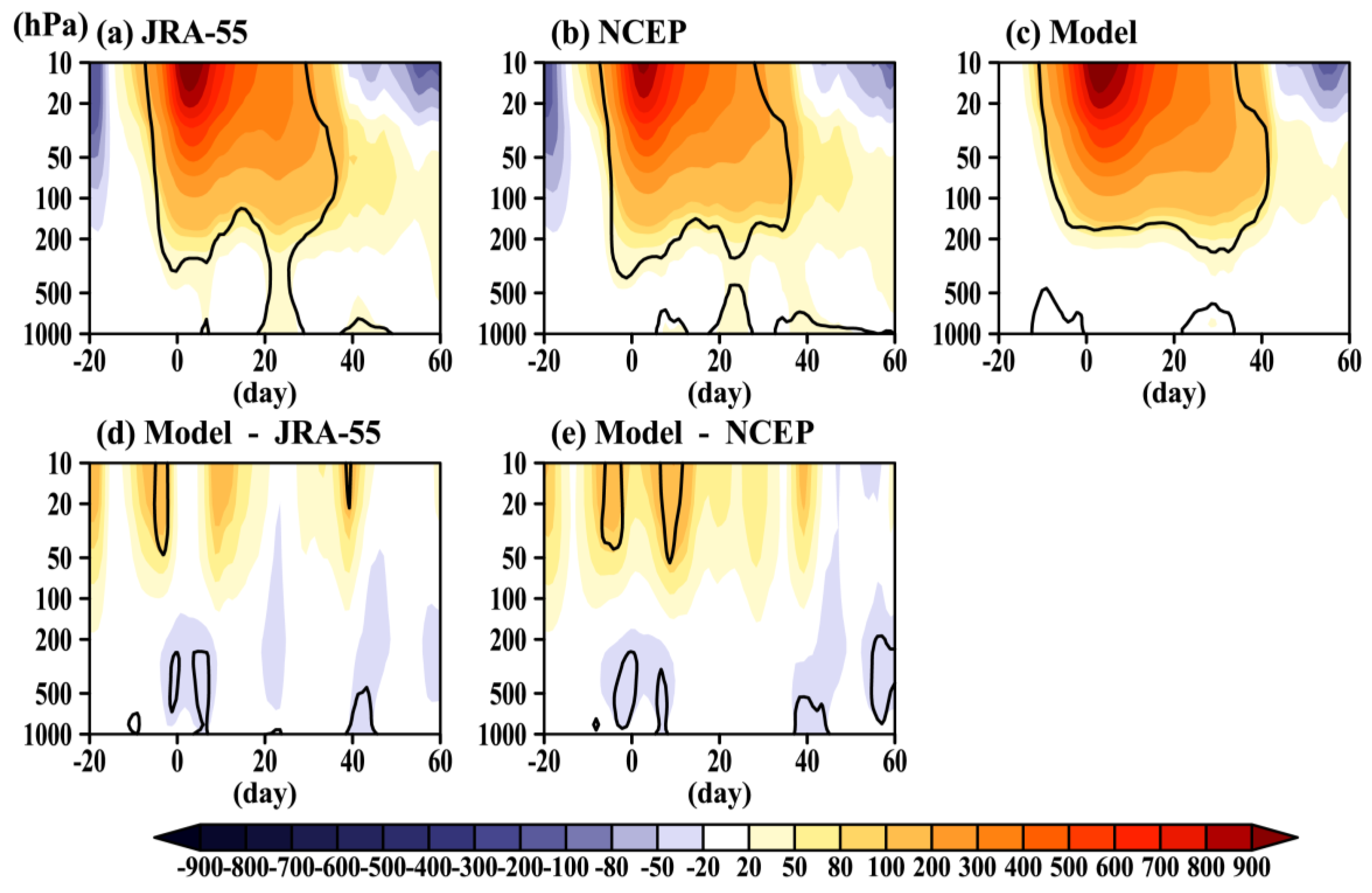
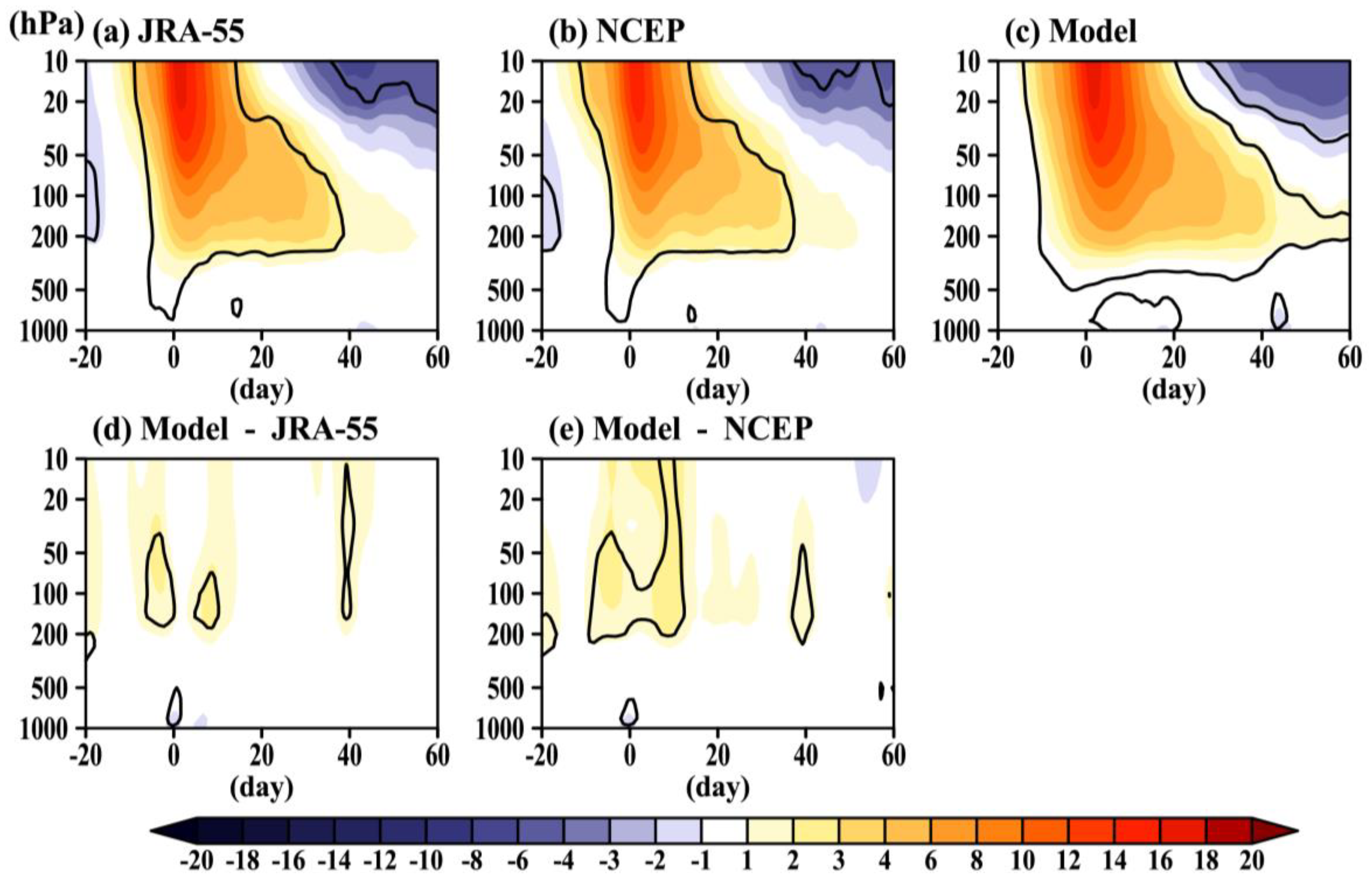
3.2. Evolution of the Stratospheric Circulation and Temperature During SSW

In order to evaluate the reproducibility of SSW events, three indicators are calculated, including the zonal wind in the circumpolar region (55–75° N), the polar cap temperature (60–90° N), and the polar cap geopotential height (60–90° N) area-averaged over the specified areas. The composite pressure–time evolution from day −20 to day 60 with respect to the SSW onset date is shown in Figure 4 for the JRA55, NCEP/NCAR reanalysis and CESM1-WACCM.
Comparing the zonal mean zonal wind around the SSW onset date, it can be seen that the composite evolution of SSW events in the reanalysis is successfully reproduced by the model. Specifically, the easterly wind anomalies in observations (Figure 4a,b) rapidly strengthen from the upper stratosphere and reach maxima (30 m/s in JRA55, 25 m/s in NCEP/NCAR) at 10 h Pa after the SSW onset. Similarly, the easterly anomalies in the stratosphere also reach maxima (30 m/s) after the SSW onset in CESM1-WACCM (Figure 4c). The easterly wind anomaly stronger than 10 m/s maintains nearly a month after the SSW onset in both reanalyses (Figure 4a,b), which is also successfully simulated by the model (Figure 4c). From the composite difference between the model and the reanalyses (Figure 4d,e), it can be seen that the wind biases are not statistically significant most of the time after the SSW onset. Different from the WACCM early version (version 3.5) showing an overestimated persistence of SSW signals [63], the persisting time of SSWs in CESM1-WACCM (version 4) largely resembles the reanalyses. It can be seen that the negative wind anomalies propagate downward to the near surface after the SSW onset in both reanalyses and the models. Unlike the strong and uniform wind anomalies in the stratosphere, the near surface winds fluctuate after the SSW onset, which might be caused by the tropospheric internal variability [64].
According to the geostrophic wind principle, the reversal of zonal wind is connected with the rise of polar cap geopotential height. The composite evolutions of the polar cap height anomalies are shown in Figure 5. Consistent with the evolution of zonal mean zonal wind anomalies in Figure 4, the positive height anomalies begin to develop several days before the SSW onset in both the model and the reanalyses (Figure 5a–c). The positive height anomalies in the upper stratosphere from the both reanalyses gradually develop deep in the stratosphere and reach the near surface 2–3 weeks after the SSW onset (Figure 5a,b). Positive height anomalies are also identified 2–3 weeks after the SSW onset in the model (Figure 5c). The positive height anomalies in the upper stratosphere reverse to negative anomalies about one month after the SSW onset in the two reanalyses, which is also well simulated by the model. The positive height anomalies in the upper troposphere and lower stratosphere can persist more than one and half months in all datasets. Therefore, the height biases, as measure by the model minus the reanalyses difference, are not statistically significant most of the time (Figure 5d,e).
Another noticeable feature for SSW events is an abrupt increase in the polar cap temperature [2,9,53]. The composite evolutions of the polar cap temperature anomalies are shown in Figure 6. Different from the positive height anomalies in the stratosphere polar cap that descend to the near surface, the warm temperature anomalies only descend to the upper troposphere with weak cold temperature anomalies in the lower troposphere and near surface (Figure 6a–c). The significant warm temperature anomalies develop from several days before the SSW onset to weeks after the SSW onset both in the reanalyses and in the model (Figure 6a–c). The maximum warm temperature anomalies reach above 14–16 K in the reanalyses around the SSW onset date (Figure 6a,b), which is well reproduced by the model (Figure 6c). For most of the SSW lifetime, the temperature anomaly bias in the troposphere is weak and non-significant, confirming the good representation of SSW events in the model (Figure 6d,e).

3.3. Evolution of Tropospheric Circulation During SSW Events

Previous studies reported that occurrence of SSWs is caused by the amplification and vertical propagation of planetary waves originating in the troposphere while recent studies [65] have suggested tropospheric wave forcing may only play a role in about 30% of SSWs. Planetary waves propagate upward to affect the stratospheric circulation and interact with the background mean currents [6,9,19,20]. To well understand the tropospheric wave source or the so-called tropospheric precursor before SSW events and the tropospheric response after the SSW onset, evolutions of the 10-day mean extratropical geopotential height anomalies at 500 h Pa are shown in Figure 7.
It can be observed by visual inspection that significant negative height anomalies are centered over the North Pacific 15–25 days before the SSW onset, while Arctic Canada and Russia are covered with positive height anomalies, which is fairly similar to a PNA pattern in its positive phase [55]. The negative height anomaly center over the North Pacific is in phase with the climatological trough there and can also be projected into the negative WP pattern [56,57]. The height anomaly patterns in the reanalyses (Figure 7(a1,b1)) amplify the climatological planetary waves, corresponding to enhanced wave activity [15,25,66]. The negative height anomaly center over the North Pacific, the positive center over Canada, and another negative center over the East US still persist from day −15 to day −5 (Figure 7(a2,b2)). Namely, the positive PNA-like pattern is still clearly presented, although only the negative center over the North Pacific is significant at the 95% confidence level. The PNA-like pattern largely weakens from day −5 to day 5, and a negative NAO-like pattern forms due to the downward propagation of the SSW signals and their impact on the troposphere [58] (Figure 7(a3,b3)). When a negative NAO forms, negative pressure (height) anomalies appear in midlatitudes of the Atlantic sector in the Northern Hemisphere, and positive pressure (height) anomalies appear in the high-latitudes of the North Atlantic and the Arctic Ocean. The low pressure (or negative height) anomalies in Eurasia usually persist a long time due to the gradual propagation of the circulation anomalies following SSW events (Figure 7(a4,a5,b4,b5)). In general, the negative height anomaly center over the North Pacific, as well as the positive PNA-like and negative WP-like patterns, is well simulated before SSW onset by the model (Figure 7(c1,c2)). However, the amplitude of height anomalies in the model is usually much stronger than in the reanalyses. Additionally, the negative NAO-like response in the North Atlantic following SSWs is shown to be stronger in the model (Figure 7(c3–c5)).

3.4. Teleconnections and Upward Propagation of Planetary Waves from the Troposphesre

Recent studies have shown that the weakening of the stratospheric polar vortex and the changing of temperature in stratosphere polar cap are closely associated with planetary wave activities originating from the extratropical troposphere [15,25,66,67,68,69], which can be confirmed by some teleconnections. Evidences show that teleconnections such as WP and PNA patterns precede SSWs while the regional pressure and temperature can be anomalously large due to the downward impact of SSW events. For example, the NAO oscillation is usually developing toward its negative phase, when the downward propagation of the AO/NAM signals during SSW events can reach the troposphere and surface [2,11,20,64]. Therefore, several selected teleconnections are calculated from day −50 to day 50 so as to evaluate the tropospheric precursor and “follower” for SSWs in the model.
The day-to-day evolutions of the PNA, WP, and NAO indices are shown in Figure 8. Firstly, the negative WP phase is observed before SSW events, which is quite persistent before SSW onset (Figure 8a–c). Secondly, the PNA from the reanalyses fluctuates fairly frequently, although it is mainly in its positive phase before the SSW onset (Figure 8a,b). Thirdly, during the time evolution of NAO from day −30 to day 30, the NAO is dominated by its negative phase throughout SSWs (Figure 8a,b). Those observational facts can be well simulated by the model: the pre-SSW period is also mainly controlled by the positive PNA and negative WP in the model; the NAO is in its negative phase for most part of the focused period from day −30 to day 30 in the model and it seems to be more significantly negative in the model especially after SSWs (Figure 8c), consistent with Figure 7(c3–c5). It can also be observed that the changes related to WP pattern are more consistent and significant in both the reanalyses and the model than the NAO response.
Since the upward propagation of planetary waves (i.e., the vertical component of the Eliassen-Palm flux, Fz) is almost proportional to the eddy heat flux ( v T ¯ ), the eddy heat flux can measure the upward propagation of waves [2,9,15,28,58]. The pressure-time evolutions of eddy heat flux area-averaged over 45°–75° N from day −40 to day 40 are shown in Figure 9. It is obvious that poleward (positive) eddy heat flux anomalies reach maxima several days before the SSW onset, and their signs are changed soon after the SSW onset, implying that the upward propagation of planetary waves is prohibited under the stratospheric easterly wind background in the mid-to-high latitudes for both the reanalyses (Figure 9a,b) and the model (Figure 9a–c). Enhanced upward propagation of waves before SSWs is well simulated in the model: the maximum eddy heat flux anomaly at 10 h Pa is nearly the same as in the JRA55 reanalysis (>80 K m/s; Figure 9a,c). The well simulated wave activities before SSWs can also be seen from the 10 h Pa eddy heat flux (Figure 9d). The timing of the eddy heat flux peaks for SSW events are well simulated by CESM1-WACCM. The negative eddy heat flux following the SSW onset implies an anomalous downward propagation of waves, when the downward impact of SSWs is strong.

3.5. Downward Impact of SSW

Figure 10 shows the evolution of the 850 h Pa air temperature anomalies in the northern extratropics during SSW to explicitly demonstrate the impact of SSWs. It should be noticed that no model data is available in Tibet Plateau, Greenland and Rocky Mountains because of high altitudes in those regions. The temperature anomaly patterns before SSW onset (left two columns in Figure 10) is mainly related to the development of positive PNA and negative WP, as well as the negative NAO. The evolution of temperature anomalies in the following periods (right three columns in Figure 10) is caused by the downward impact of SSW events.
Specifically, it can be observed by visual inspection from the reanalyses that warm conditions appear in the North American continent from day −25 to day −15, while the North Eurasian continent is covered with cold anomalies (Figure 10(a1,b1)). This temperature pattern still persists from day −15 to day −5 in the reanalysis (Figure 10(a2,b2)). From day −5 to day 5, the cold North Eurasia–warm North America pattern is still clear in mid-to-high latitudes, while the lower latitudes of Eurasia are anomalously warm and the lower latitudes of North America are cold (Figure 10(a3,b3)). The warm anomalies in the North America weaken gradually and are replaced by cold anomalies from day 5 to day 15 (Figure 10(a4,b4)). Finally, the continents in mid-to-high latitudes are mostly covered with cold anomalies (Figure 10(a5,b5)). The model can well capture the evolutions of 850 h Pa temperature anomalies (Figure 10b), including the cold Eurasia–warm North America pattern before SSW onset (Figure 10(c1,c2)) and cold Eurasia–cold North America following SSWs (Figure 10(c3–c5)). Comparing the reanalyses and the model, it is revealed that areas covered with significant temperature anomalies in the model are wider than those in the reanalyses, which might be caused by the anomalously strong NAO pattern in the model (Figure 7c).

4. Summary and Discussion

This study assessed the CESM1-WACCM model in simulating the SSW events and their downward impact based on the JRA55 and NCEP/NCAR reanalyses. A detailed statistical and diagnostic analysis of SSW events were carried out for a historical run by CESM1-WACCM, the JRA55 reanalysis and the NCEP/NCAR reanalysis. Those diagnoses include the statistical distribution of SSW events in every decade and every month, the primary biases of SSWs in the model historical run with respect to the reanalyses and the representation of the tropospheric precursor for SSWs in the model. The main findings in the study are as follow.
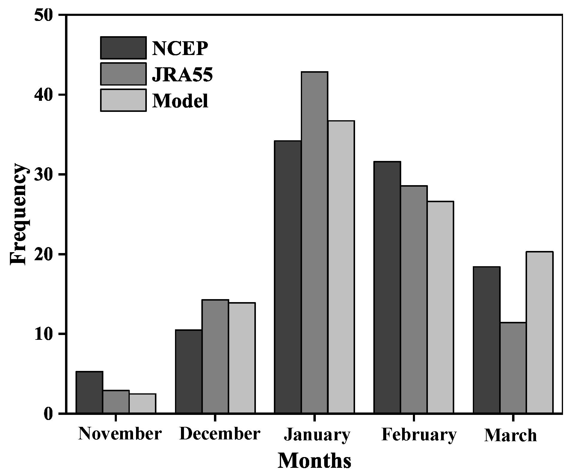
  • On average, major SSW events based on the WMO definition [8] occur 5–6 times per decade in the JRA55 and NCEP/NCAR reanalyses, which is realistically reproduced by CESM1-WACCM. The seasonal distribution of SSWs in wintertime is also well simulated, although some tiny differences between the reanalyses and the model are noticed. The SSW events in January ranks the first in the percentage (35%), followed by February; while SSW events in November ranks the last in the percentage, which is also realistically reproduced by the model. Considering the large uncertainty from the reanalyses (especially NCEP/NCAR) and the large variability in the stratosphere, the different SSW occurrence percentages between the reanalyses and the model for some months (December and March) may not indicate a poor representation of SSW events in the model. In general, the SSW percentage in midwinter from the model falls between the two reanalyses.
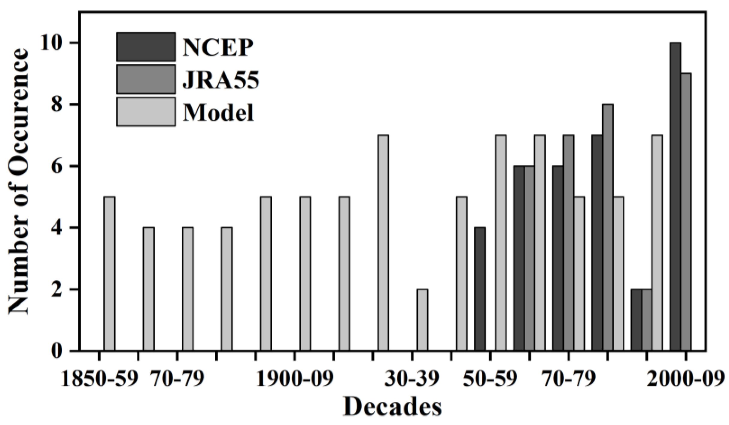
  • The SSW absence observed in 1990s from the reanalysis can also be identified in the model data, but of a different model decade (1930s). The scarcity of SSW events in some decades might reflect the internal variability of the stratosphere. Because the historical run is an “atmosphere-ocean coupled run” experiment, the SST and sea ice are generated by the model. Therefore, the model shows a different SSW number from the reanalyses in every decade.
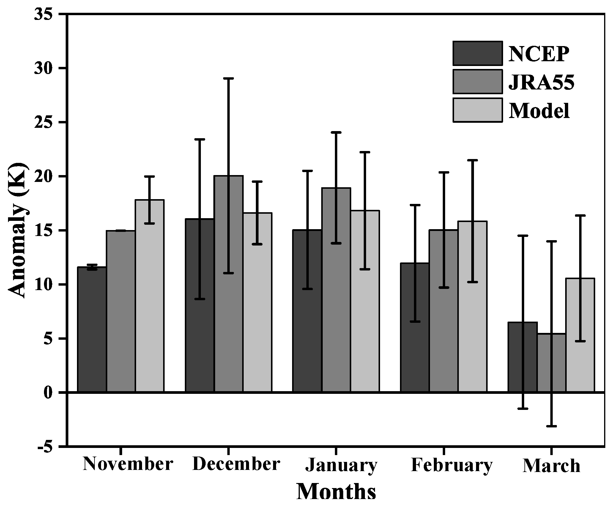
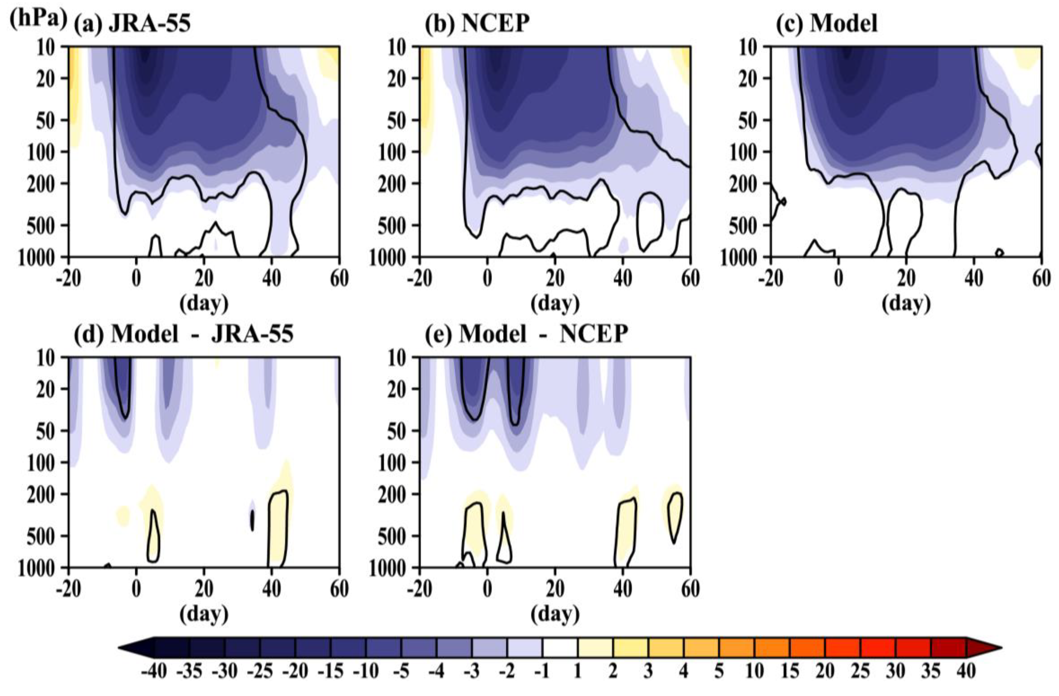
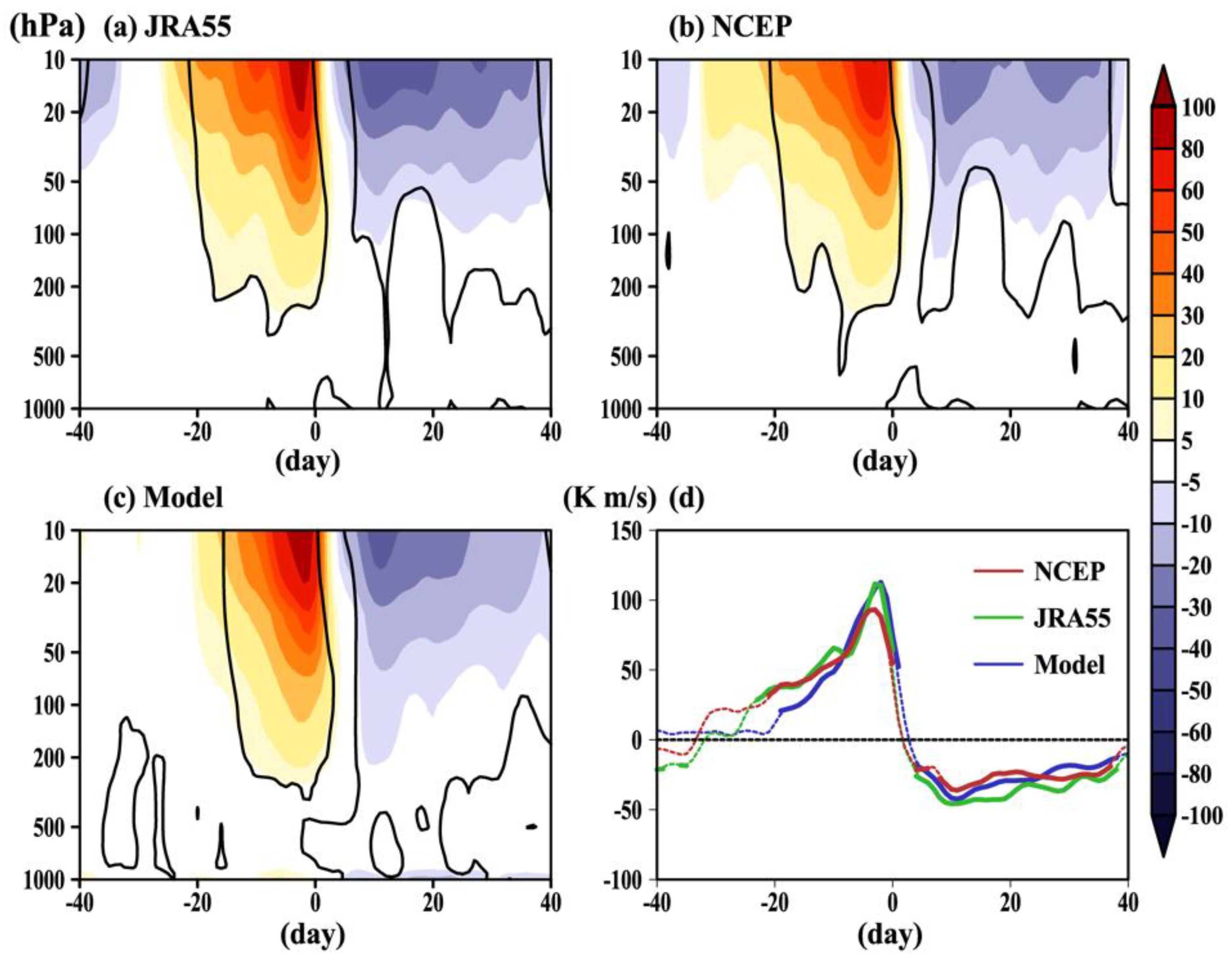
  • The SSW intensity measured by the circumpolar easterly anomalies, the polar cap temperature anomalies, and polar cap height anomalies are nicely simulated. The overestimated duration of SSW events in an earlier WACCM version (WACCM3.5 [63]) is not seen in this version (WACCM4). Further, the model can well reproduce the downward propagation of easterly anomalies and the negative NAM represented by the positive polar cap height anomalies following the SSW onset. The polar cap warm temperature anomalies propagate from the upper stratosphere to the upper troposphere in all datasets. The enhanced wave activities evaluated by the eddy heat flux before the SSW onset are also realistically reproduced, and the suppressed wave activities after the SSW onset are fairly similar in the reanalyses and the model.
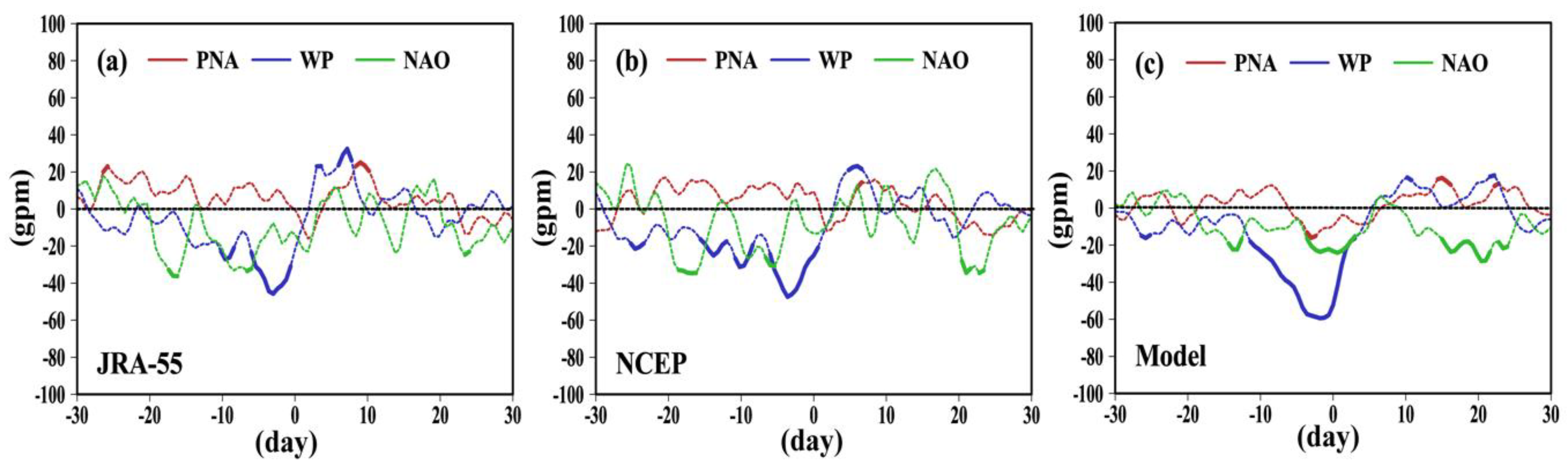
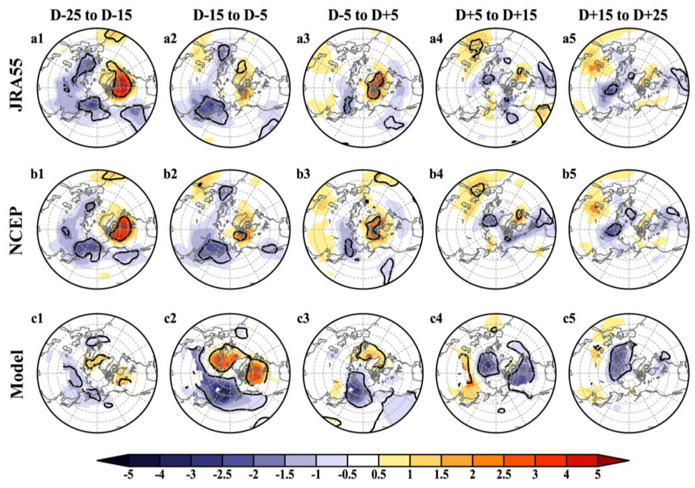
  • Both the modelling and observational evidences indicate that SSWs are proceeded by the positive PNA and negative WP pattern in the troposphere, which favor the amplification and upward propagation of extratropical waves in pre-SSW periods. The model can well simulate the negative WP pattern and the positive PNA pattern before SSWs. The negative NAO develops throughout the SSW life cycle, which is simulated to be more significantly negative in the model after SSWs, and the NAO response is seemingly weaker than that of the WP pattern.
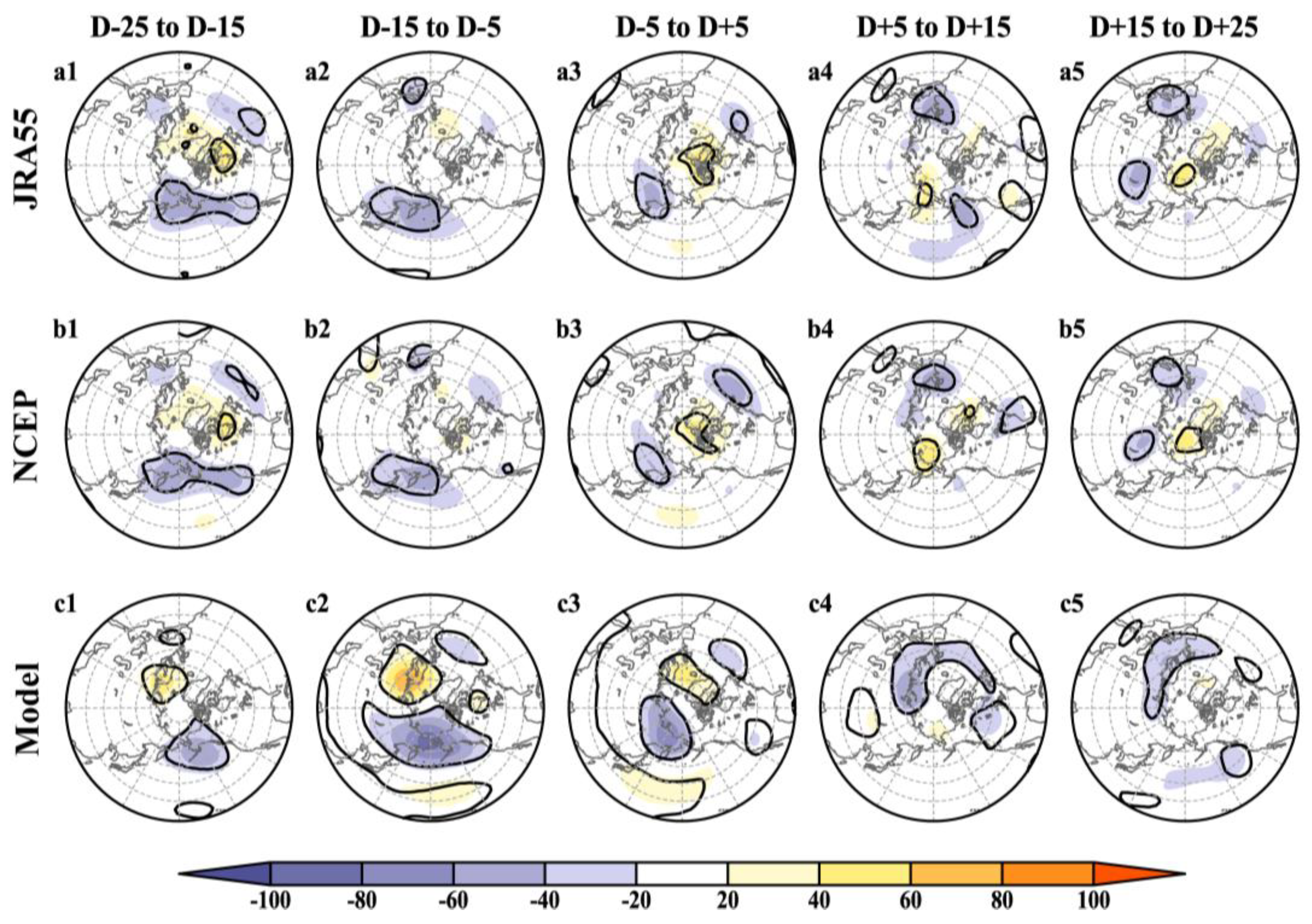
  • A cold Eurasian continent–warm North American continent pattern is observed in some pre-SSW periods, while the two continents are anomalously cold in some post-SSW periods. The model can produce distribution of the 850 h Pa temperature anomalies before and after the SSW onset, including the cold Eurasia–warm North America pattern before SSW onset and cold Eurasia–cold North America following SSWs.
This study systematically evaluates the model performance of CESM1-WACCM in simulating SSWs and their surface impact. Some studies show that the frequency of SSW events might be different between different phases of ENSO [18,26,58]. We still do not know if the SSW frequency in CESM1-WACCM is controlled by ENSO, which deserves further investigation. Peters et al. [29] designed two experiments, one forced by zonal mean ozone, the other forced by zonally asymmetric ozone; they that the number of SSWs in the latter experiment is larger than that in the former. The historical run in this study includes fully interactive chemistry to produce zonally asymmetric ozone, so the frequency of SSWs is nearly as high as in the JRA55 and NCEP/NCAR reanalyses. Only one model is used in this study, but CESM1-WACCM is one of the most widely used and best stratosphere-resolving models [26,43,44,45]. Since only one realization of WACCM is used in this study, the robustness of this study will be improved if more realizations are evaluated. The QBO is nudged in the CESM1-WACCM historical run, which is shown to have an impact on the northern winter stratospheric polar vortex [22,23,24,25]. The newer version of CESM-WACCM, CESM2-WACCM, has a spontaneously generated QBO, which might further improve the simulation of SSWs in this model. A comparison between the two versions of CESM-WACCM is another interesting topic beyond the limited scope of this paper. A more comprehensive comparison between different SSW types also deserves further investigation in the future work.
Only two reanalyses are used in this study, but the SSW events especially in the satellite era, have been shown to be fairly consistent between several reanalyses [61]. Furthermore, comparisons between CESM1-WACCM and other models are still lack, although the SSW modeling in MPI-ESM-LR is also reported [70]. Previous studies also emphasized that the persistence time of SSWs is very different between strong polar night jet oscillation events and weak polar night jet oscillation events [29,70], which is beyond the scope of this study but worth a deep investigation using outputs from the state-of-the-art CMIP6 models.

Author Contributions

Conceptualization, J.R. and S.-M.L.; methodology, Y.-H.C. and C.C.; software, C.C. and Y.-H.C.; validation, J.R. and S.-M.L.; formal analysis, S.-M.L. and J.R.; investigation, Y.-H.C and S.-Y.L.; writing—original draft preparation, S.-M.L and S.-Y.L.; writing—review and editing, J.R.; visualization, M.-H.M. and Y.-B.W.; supervision, J.R.; project administration, S.-M.L. and C.C.

Funding

This work was jointly supported by grants from the National Natural Science Foundation of China (41705024), the National Key R&D Program of China (2016YFA0602104), and College Student’s Practice Innovation Training Program of Jiangsu Province (201810300009Z).

Acknowledgments

We acknowledge the JRA55 and NCEP/NCAR for providing the reanalysis data. The CESM1-WACCM historical run was provided by CMIP and NCAR upon request.

Conflicts of Interest

The authors declare no conflict of interest.

References

  1. O’Neill, A.; Charlton-Perez, A.J.; Polvani, L.M. Stratospheric sudden warmings. In Encyclopedia of Atmospheric Science, 2nd ed.; North, G.R., Pyle, J., Zhang, F., Eds.; Elsevier: London, UK, 2014; Volume 4, pp. 30–40. [Google Scholar]
  2. Limpasuvan, V.; Thompson, D.W.J.; Hartmann, D.L. The life cycle of the Northern Hemisphere sudden stratospheric warmings. J. Clim. 2004, 17, 2584–2596. [Google Scholar] [CrossRef]
  3. Manney, G.L.; Krnney, G.; Sabutis, J.L.; Sena, S.A.; Pawson, S. The remarkable 2003–2004 winter and other recent warm winters in the Arctic stratosphere since the late 1990s. J. Geophys. Res. 2005, 110, 583–595. [Google Scholar] [CrossRef]
  4. Shi, C.; Xu, T.; Guo, D.; Pan, Z. Modulating effects of planetary wave 3 on a stratospheric sudden warming event in 2005. J. Atmos. Sci. 2017, 74, 1549–1559. [Google Scholar] [CrossRef]
  5. Scherhag, R. Die explosionsartigen Stratospherenerwarmingen des Spatwinters, 1951–1952. Ber. Deut. Wetterd. 1952, 6, 51–63. [Google Scholar]
  6. Matsuno, T. A dynamical model of the stratospheric sudden warming. J. Atmos. Sci. 1971, 28, 1479–1494. [Google Scholar] [CrossRef]
  7. McIntyre, M.E. How well do we understand the dynamics of stratospheric warming? J. Meteorol. Soc. Jpn. 1982, 60, 37–64. [Google Scholar] [CrossRef]
  8. Andrews, D.G.; Holton, J.R.; Leovy, C.B. Middle Atmosphere Dynamics; Academic Press: Cambridge, MA, USA, 1985; 489p. [Google Scholar]
  9. Charlton, A.J.; Polvani, L.M. A new look at stratospheric sudden warmings. Part I: Climatology and modeling benchmarks. J. Clim. 2007, 20, 449–469. [Google Scholar] [CrossRef]
  10. Limpasuvan, V.; Hartmann, D.L. Eddies and the annular modes of climate variability. Geophys. Res. Lett. 1999, 26, 3133–3136. [Google Scholar] [CrossRef] [Green Version]
  11. Black, R.X. Stratospheric forcing of surface climate in the Arctic Oscillation. J. Clim. 2002, 15, 268–277. [Google Scholar] [CrossRef]
  12. Karpechko, A.Y.; Charlton-Perez, A.; Balmaseda, M.; Tyrrell, N.; Vitart, F. Predicting sudden stratospheric warming 2018 and its climate impacts with a multi-model ensemble. Geophys. Res. Lett. 2018, 45, 13538–513546. [Google Scholar] [CrossRef]
  13. Kim, Y.J.; Flatau, M. Hindcasting the January 2009 Arctic sudden stratospheric warming and its influence on the Arctic Oscillation with unified parameterization of orographic drag in NOGAPS. Part I: Extended-range stand-alone forecast. Weather Forecast. 2010, 25, 1628–1644. [Google Scholar] [CrossRef]
  14. Dörnbrack, A.; Pitts, M.C.; Poole, L.R.; Orsolini, Y.J.; Nishii, K.; Nakamura, H. The 2009–2010 Arctic stratospheric winter–general evolution, mountain waves and predictability of an operational weather forecast model. Atmos. Chem. Phys. 2012, 12, 3659–3675. [Google Scholar] [CrossRef]
  15. Rao, J.; Ren, R.; Chen, H.; Yu, Y.; Zhou, Y. The stratospheric sudden warming event in February 2018 and its prediction by a climate system model. J. Geophys. Res. Atmos. 2018, 123, 13332–13345. [Google Scholar] [CrossRef]
  16. Mukougawa, H.; Sakai, H.; Hirooka, T. High sensitivity to the initial condition for the prediction of stratospheric sudden warming. Geophys. Res. Lett. 2005, 32, L08814. [Google Scholar] [CrossRef]
  17. Taguchi, M. Predictability of major stratospheric sudden warmings: Analysis results from JMA operational 1-month ensemble predictions from 2001/02 to 2012/13. J. Atmos. Sci. 2016, 73, 789–806. [Google Scholar] [CrossRef]
  18. Butler, A.H.; Polvani, L.M. El Niño, La Niña, and stratospheric sudden warmings: A reevaluation in light of the observational record. Geophys. Res. Lett. 2011, 38, L13807. [Google Scholar] [CrossRef]
  19. Yoden, S.; Yamaga, T.; Pawson, S.; Langematz, U. A composite analysis of the stratospheric sudden warmings simulated in a perpetual January integration of the Berlin TSM GCM. J. Meteorol. Soc. Jpn. 1999, 77, 431–445. [Google Scholar] [CrossRef]
  20. Rao, J.; Ren, R.; Chen, H.; Liu, X.; Yu, Y.; Yang, Y. Sub-seasonal to seasonal hindcasts of stratospheric sudden warming by BCC_CSM1.1(m): A comparison with ECMWF. Adv. Atmos. Sci. 2019, 35, 479–494. [Google Scholar] [CrossRef]
  21. Rao, J.; Ren, R. Varying stratospheric responses to tropical Atlantic SST forcing from early to late winter. Clim. Dyn. 2018, 51, 2079–2096. [Google Scholar] [CrossRef]
  22. Rao, J.; Yu, Y.; Guo, D.; Shi, C.; Chen, D.; Hu, D. Evaluating the Brewer–Dobson circulation and its responses to ENSO, QBO, and the solar cycle in different reanalyses. Earth Planet. Phys. 2019, 3, 166–181. [Google Scholar] [CrossRef]
  23. Holton, J.R.; Tan, H.C. The Influence of the equatorial quasi-biennial oscillation on the global circulation at 50mb. J. Atmos. Sci. 1980, 37, 2200–2208. [Google Scholar] [CrossRef]
  24. Naito, Y.; Taguchi, M.; Yoden, S. A parameter sweep experiment on the effects of the equatorial QBO on stratospheric sudden warming events. J. Atmos. Sci. 2003, 60, 1380–1394. [Google Scholar] [CrossRef]
  25. Garfinkel, C.I.; Hartmann, D.L. Effects of the El Niño–Southern oscillation and the quasi-biennial oscillation on polar temperatures in the stratosphere. J. Geophys. Res. 2007, 112, D19112. [Google Scholar] [CrossRef]
  26. Taguchi, M.; Hartmann, D.L. Increased occurrence of stratospheric sudden warmings during El Niño as simulated by WACCM. J. Clim. 2006, 19, 324–332. [Google Scholar] [CrossRef]
  27. Wei, K.; Chen, W.; Huang, R.H. Association of tropical Pacific sea surface temperatures with the stratospheric Holton-Tan Oscillation in the Northern Hemisphere winter. Geophys. Res. Lett. 2007, 34, L16814. [Google Scholar] [CrossRef]
  28. Rao, J.; Ren, R. Parallel comparison of the 1982/83, 1997/98 and 2015/16 super El Niños and their effects on the extratropical stratosphere. Adv. Atmos. Sci. 2017, 34, 1121–1133. [Google Scholar] [CrossRef]
  29. Peters, D.H.W.; Schneidereit, A.; Bügelmayer, M.; Zülicke, C.; Kirchner, I. Atmospheric circulation changes in response to an observed stratospheric zonal ozone anomaly. Atmos. Ocean 2014, 53, 74–88. [Google Scholar] [CrossRef]
  30. Baldwin, M.P.; Dunkerton, T.J. Propagation of the Arctic Oscillation from the stratosphere to the troposphere. J. Geophys. Res. 1999, 104, 30937–30946. [Google Scholar] [CrossRef]
  31. Baldwin, M.P.; Stephenson, D.B.; Thompson, D.W.J.; Dunkerton, T.J.; Charlton, A.J.; O’Nell, A. Stratospheric memory and skill of extended-range weather forecasts. Science 2003, 301, 636–640. [Google Scholar] [CrossRef]
  32. Thompson, D.W.J.; Wallace, J.M. Annular modes in the extratropical circulation. Part I: Month-to-month variability. J. Clim. 2000, 13, 1000–1016. [Google Scholar] [CrossRef]
  33. Thompson, D.W.J.; Baldwin, M.P.; Wallace, J.M. Stratospheric connection to Northern Hemisphere wintertime weather: Implications for prediction. J. Clim. 2002, 15, 1421–1428. [Google Scholar] [CrossRef]
  34. Stan, C.; Straus, D.M. Stratospheric predictability and sudden stratospheric warming events. J. Geophys. Res. 2009, 114, D12103. [Google Scholar] [CrossRef]
  35. Roff, G.; Thompson, D.W.J.; Hendon, H. Does increasing model stratospheric resolution improve extended-range forecast skill? Geophys. Res. Lett. 2011, 38, L05809. [Google Scholar] [CrossRef]
  36. Tripathi, O.P.; Baldwin, M.; Charlton-Perez, A.; Charron, M.; Eckermann, S.D.; Gerber, E.; Harrison, G.; Jackson, D.R.; Kim, B.-M.; Kuroda, Y.; et al. The predictability of the extratropical stratosphere on monthly time-scales and its impact on the skill of tropospheric forecasts. Q. J. R. Meteorol. Soc. 2015, 141, 987–1003. [Google Scholar] [CrossRef]
  37. Allen, D.R.; Coy, L.; Eckermann, S.D.; McCormack, J.P.; Manney, G.L.; Hogan, T.F.; Kim, Y.J. NOGAPS-ALPHA simulations of the 2002 Southern Hemisphere stratospheric major warming. Mon. Weather Rev. 2006, 134, 498–518. [Google Scholar] [CrossRef]
  38. Kim, Y.J.; Campbell, W.; Ruston, B. Hindcasting the January 2009 Arctic sudden stratospheric warming and its influence on the Arctic oscillation with unified parameterization of orographic drag in NOGAPS. Part II: Short-range data-assimilated forecast and the impacts of calibrated radiance bias correction. Weather Forecast. 2011, 26, 993–1007. [Google Scholar]
  39. Taguchi, M. Predictability of major stratospheric sudden warmings of the vortex split type: Case study of the 2002 southern event and the 2009 and 1989 northern events. J. Atmos. Sci. 2014, 71, 2886–2904. [Google Scholar] [CrossRef]
  40. Tripathi, O.P.; Baldwin, M.; Charlton-Perez, A.; Charron, M.; Cheung, J.C.H.; Eckermann, S.D.; Gerber, E.; Jackson, D.R.; Kuroda, Y.; Lang, A.; et al. Examining the predictability of the stratospheric sudden warming of January 2013 using multiple NWP systems. Mon. Weather Rev. 2016, 144, 1935–1960. [Google Scholar] [CrossRef]
  41. Simmons, A.; Hortal, M.; Kelly, G.; McNally, A.; Untch, A.; Uppala, S. ECMWF analyses and forecasts of stratospheric winter polar vortex breakup: September 2002 in the Southern Hemisphere and related events. J. Atmos. Sci. 2005, 62, 668–689. [Google Scholar] [CrossRef]
  42. Hirooka, T.; Ichimaru, T.; Mukougawa, H. Predictability of stratospheric sudden warmings as inferred from ensemble forecast data: Intercomparison of 2001/02 and 2003/04 winters. J. Meteorol. Soc. Jpn. 2007, 85, 919–925. [Google Scholar] [CrossRef]
  43. Rao, J.; Ren, R.C.; Yang, Y. Parallel comparison of the northern winter stratospheric circulation in reanalysis and in CMIP5 models. Adv. Atmos. Sci. 2015, 32, 952–966. [Google Scholar] [CrossRef]
  44. Gent, P.R.; Danabasoglu, G.; Donner, L.J.; Holland, M.M.; Hunke, E.C.; Jayne, S.R.; Lawrence, D.M.; Neale, R.B.; Rasch, P.J.; Vertenstein, M.; et al. The Community Climate System Model version 4. J. Clim. 2011, 24, 4973–4991. [Google Scholar] [CrossRef]
  45. Marsh, D.R.; Mills, M.J.; Kinnison, D.E.; Lamarque, J.F.; Calvo, N.; Polvani, L.M. Climate change from 1850 to 2005 simulated in CESM1(WACCM). J. Clim. 2013, 26, 7372–7391. [Google Scholar] [CrossRef]
  46. Ren, R.C.; Rao, J.; Wu, G.X.; Cai, M. Tracking the delayed response of the northern winter stratosphere to ENSO using multi reanalyses and model simulations. Clim. Dyn. 2017, 48, 2859–2879. [Google Scholar] [CrossRef]
  47. Richter, J.H.; Sassi, F.; Garcia, R.R. Toward a physically based gravity wave source parameterization in a general circulation model. J. Atmos. Sci. 2010, 67, 136–156. [Google Scholar] [CrossRef]
  48. Kalnay, E.; Kanamitsu, M.; Kistler, R.; Collins, W.; Deaven, D.; Gandin, L.; Iredell, M.; Saha, S.; White, G.; Woollen, J.; et al. The NCEP/NCAR 40-year reanalysis project. Bull. Am. Meteorol. Soc. 1996, 77, 437–471. [Google Scholar] [CrossRef]
  49. Kobayashi, S.; Ota, Y.; Harada, Y.; Ebita, A.; Moriya, M.; Onoda, H.; Onogi, K.; Kamahori, H.; Kobayashi, C.; Endo, H.; et al. The JRA-55 reanalysis: General specifications and basic characteristics. J. Meteorol. Soc. Jpn. 2015, 93, 5–48. [Google Scholar] [CrossRef]
  50. Martineau, P.; Son, S.-W.; Taguchi, M.; Butler, A.H. A comparison of the momentum budget in reanalysis datasets during sudden stratospheric warming events. Atmos. Chem. Phys. 2018, 18, 7169–7187. [Google Scholar] [CrossRef] [Green Version]
  51. Gerber, E.P.; Martineau, P. Quantifying the variability of the annular modes: Reanalysis uncertainty vs. sampling uncertainty. Atmos. Chem. Phys. 2018, 18, 17099–17117. [Google Scholar] [CrossRef]
  52. Rao, J.; Ren, R.; Xia, X.; Shi, C.; Guo, D. Combined impact of El Niño–Southern Oscillation and Pacific Decadal Oscillation on the northern winter stratosphere. Atmosphere 2019, 10, 211. [Google Scholar] [CrossRef]
  53. Butler, A.H.; Seidel, D.J.; Hardiman, S.C.; Butchart, N.; Birner, T.; Match, A. Defining sudden stratospheric warmings. Bull. Am. Meteorol. Soc. 2015, 96, 1913–1928. [Google Scholar] [CrossRef]
  54. Thiéblemont, R.; Ayarzagüena, B.; Matthes, K.; Bekki, S.; Abalichin, J.; Langematz, U. Drivers and surface signal of interannual variability of boreal stratospheric final warmings. J. Geophys. Res. Atmos. 2019, 124, 5400–5417. [Google Scholar] [CrossRef]
  55. Rao, J.; Ren, R. A decomposition of ENSO’s impacts on the northern winter stratosphere: Competing effect of SST forcing in the tropical Indian Ocean. Clim. Dyn. 2016, 46, 3689–3707. [Google Scholar] [CrossRef]
  56. Dai, Y.; Tan, B.K. The western Pacific pattern precursor of major stratospheric sudden warmings and the ENSO modulation. Environ. Res. Lett. 2016, 11, 124032. [Google Scholar] [CrossRef] [Green Version]
  57. Hu, J.G.; Li, T.; Xu, H.M.; Yang, S.Y. Lessened response of boreal winter stratospheric polar vortex to El Niño in recent decades. Clim. Dyn. 2017, 49, 263–278. [Google Scholar] [CrossRef]
  58. Polvani, L.M.; Sun, L.; Butler, A.H.; Richter, J.H.; Deser, C. Distinguishing stratospheric sudden warmings from ENSO as key drivers of wintertime climate variability over the North Atlantic and Eurasia. J. Clim. 2017, 30, 1959–1969. [Google Scholar] [CrossRef]
  59. Wallace, J.M.; Gutzler, D.S. Teleconnections in the geopotential height field during the northern hemisphere winter. Mon. Weather Rev. 1981, 109, 784–812. [Google Scholar] [CrossRef]
  60. Hu, J.G.; Ren, R.C.; Xu, H.M. Occurrence of winter stratospheric sudden warming events and the seasonal timing of spring stratospheric final warming. J. Atmos. Sci. 2014, 71, 2319–2334. [Google Scholar] [CrossRef]
  61. Butler, A.H.; Sjoberg, J.P.; Seidel, D.J.; Rosenlof, K.H. A sudden stratospheric warming compendium. Earth Syst. Sci. Data 2017, 9, 63–76. [Google Scholar] [CrossRef] [Green Version]
  62. Wang, H.Z.; Rao, J.; Sheng, C.; Wang, B. Statistical characteristics of the Northern Hemisphere stratospheric sudden warming and its seasonality (1948–2015). Trans. Atmos. Sci. 2019, 42. (In Chinese) [Google Scholar] [CrossRef]
  63. de la Torre, L.; Garcia, R.R.; Barriopedro, D.; Chandran, A. Climatology and characteristics of stratospheric sudden warmings in the whole atmosphere community climate model. J. Geophys. Res. Atmos. 2012, 117, D04110. [Google Scholar] [CrossRef]
  64. Baldwin, M.P.; Dunkerton, T.J. Stratospheric harbingers of anomalous weather regimes. Science 2001, 294, 581–584. [Google Scholar] [CrossRef] [PubMed]
  65. de la Cámara, A.; Birner, T.; Albers, J.R. Are sudden stratospheric warmings preceded by anomalous tropospheric wave activity? J. Clim. 2019. [Google Scholar] [CrossRef]
  66. Garfinkel, C.I.; Benedict, J.J.; Maloney, E.D. Impact of the MJO on the boreal winter extratropical circulation. Geophys. Res. Lett. 2014, 41, 6055–6062. [Google Scholar] [CrossRef]
  67. Rao, J.; Ren, R.C. Asymmetry and nonlinearity of the influence of ENSO on the northern winter stratosphere: 1. Observations. J. Geophys. Res. 2016, 121, 9000–9016. [Google Scholar] [CrossRef] [Green Version]
  68. Rao, J.; Ren, R.C. Asymmetry and nonlinearity of the influence of ENSO on the northern winter stratosphere: 2. Model study with WACCM. J. Geophys. Res. 2016, 121, 9017–9032. [Google Scholar] [CrossRef]
  69. Maycock, A.C.; Hitchcock, P. Do split and displacement sudden stratospheric warmings have different annular mode signatures? Geophys. Res. Lett. 2015, 42, 10943–10951. [Google Scholar] [CrossRef]
  70. Peters, D.H.W.; Schneidereit, A.; Karpechko, A.Y. Enhanced stratosphere/troposphere coupling during extreme warm stratospheric events with strong polar-night jet oscillation. Atmosphere 2018, 9, 467. [Google Scholar] [CrossRef]
Figure 1. The frequency distribution (units: percentage) of SSW events in each wintertime month in the NCEP/NCAR (black) and JRA55 reanalyses (dark grey) and CESM1-WACCM (light grey).
Atmosphere 10 00519 g001
Figure 2. The occurrence number of sudden stratospheric warming (SSW) events in each decade in the NCEP/NCAR (black) and JRA55 reanalyses from 1950s/1960s to 2000s (dark grey) and in CESM1-WACCM from 1850s to 2000s (light grey).
Atmosphere 10 00519 g002
Figure 3. Composite of mean area-weighted polar cap (60°–90° N) temperature anomaly at 10 h Pa, ±5 days from the SSW onset date in each wintertime month for the NCEP/NCAR (black) and JRA55 reanalyses (dark grey) and CESM1-WACCM (light grey). The error bar denotes the inter-case standard deviation.
Atmosphere 10 00519 g003
Figure 4. Composite pressure–time evolution of the zonal mean zonal wind anomalies area-averaged over 55 –75° N (shadings; units: m/s) from day −20 to day 60 relative to the SSW onset date for (a) the JRA55 reanalysis, (b) the NCEP/NCAR reanalysis, and (c) CESM1-WACCM. The last two plots (d,e) shows the difference between the model and the reanalyses. Black contours mark the composite zonal wind anomalies/differences at the 95% confidence level according to the t-test.
Atmosphere 10 00519 g004
Figure 5. Same as in Figure 4, but for the zonal mean geopotential height anomalies area-averaged over the polar cap region from 60–90° N (shadings; units: gpm).
Atmosphere 10 00519 g005
Figure 6. Same as in Figure 4, but for the polar cap temperature anomalies area-averaged over 60–90° N (shadings; units: K).
Atmosphere 10 00519 g006
Figure 7. Composite of geopotential height anomalies (shadings; units: gpm) at 500 h Pa in (a1–a5) the JRA55 reanalysis, (b1–b5) the NCEP/NCAR reanalysis, and (c1–c5) CESM1-WACCM during day −25 to −15 (first column), day −15 to −5 (second column), day −5 to 5 (middle column), day 5 to 15 (fourth column), and day 15 to 25 (fifth column) relative to the SSW onset date. Black contours indicate that the composite height anomalies are significant at the 95% confidence level according to the t-test.
Atmosphere 10 00519 g007
Figure 8. Day-to-day evolution of the PNA (red), WP (blue), and NAO (green) indices from day −30 to day 30 from (a) the JRA55 reanalysis, (b) the NCEP/NCAR reanalysis, and (c) CESM1-WACCM. Thickened solid parts of the line indicate that the composite index is significant at the 95% confidence level according to the t-test.
Atmosphere 10 00519 g008
Figure 9. Composite evolution of eddy heat flux area-averaged in the 45°–75° N latitude band from 1000–10 h Pa (shadings; units: K m/s) from day −40 to day 40 relative to the SSW onset date for (a) the JRA55 reanalysis, (b) the NCEP/NCAR reanalysis, and (c) CESM1-WACCM. Black contours indicate that the composite anomalies are significant at the 95% confidence level. The last plot (d) shows the temporal evolution of eddy heat flux at 10 h Pa (units: K m/s) from the JRA55 reanalysis (green), the NCEP/NCAR reanalysis (red) and CESM1-WACCM (blue), receptively. Thickened solid parts of the line indicate the composite is significant at the 95% confidence level according to the t-test.
Atmosphere 10 00519 g009
Figure 10. Same as in Figure 7, but for temperature anomaly distribution (shading, units: K) at 850 h Pa.
Atmosphere 10 00519 g010
Table 1. Onset dates of sudden stratospheric warmings (SSW) events in the JRA55 and NCEP/NCAR reanalyses (1958/1948–2015) and in the CESM1-WACCM historical run (1850–2005).
Date in JRA55Date in NCEP/NCARDate in CESM1-WACCM
25 February 19522 March 18517 February 1930
8 February 195720 March 185318 January 1936
****30 January 195829 December 185312 December 1941
****30 November 195810 January 185515 January 1945
17 January 196016 January 196022 March 18553 December 1947
30 January 1963****28 January 186019 February 1948
****23 March 196528 March 186228 January 1949
18 December 19658 December 196515 January 186519 March 1952
23 February 196624 February 196619 March 18676 January 1953
7 February 1968****26 January 187418 March 1953
29 November 196827 November 196813 January 187617 March 1954
****13 March 196917 January 187720 February 1955
2 January 19702 January 19706 December 187724 January 1958
25 January 197025 January 19704 January 188014 January 1959
18 January 197117 January 19714 February 188021 February 1960
20 March 197120 March 197119 February 188727 November 1961
31 January 19732 February 197313 January 188918 February 1963
9 January 1977****4 February 188931 January 1964
22 February 197922 February 19793 March 189319 March 1965
29 February 198029 February 198023 November 189428 December 1966
6 February 1981****26 December 18967 February 1969
4 December 19814 December 198124 January 18986 January 1970
1 January 19852 January 198521 December 189917 February 1971
23 January 198723 January 198730 January 19009 March 1973
8 December 19878 December 198722 March 190119 January 1977
14 March 198814 March 19886 January 19047 January 1979
21 February 198922 February 198929 January 19064 February 1981
15 December 199815 December 199826 January 190826 January 1985
26 February 199925 February 199921 January 19103 February 1986
20 March 200020 March 20007 February 19122 March 1987
11 February 200111 February 200110 February 191427 February 1989
31 December 20012 January 20029 February 191526 March 1993
18 January 200318 January 200324 December 191712 January 1994
5 January 20047 January 200418 February 192025 February 1994
21 January 200621 January 200620 March 192018 February 1995
24 February 200724 February 200716 December 19206 March 1997
22 February 200822 February 200822 January 19228 February 1998
****14 March 20088 December 192410 January 1999
24 January 200924 January 200919 March 19289 February 2003
9 February 20109 February 20101 January 192914 January 2005
24 March 201024 March 2010
7 January 20137 January 2013
The asterisk signs (****) in the left two columns indicate that an SSW event is not identified in one of the two reanalyses, but is identified in the other.

