Article

Fetch Effect on Flux-Variance Estimations of Sensible and Latent Heat Fluxes of Camellia Sinensis

1
School of Agricultural Equipment Engineering, Jiangsu University, Zhenjiang 212013, China
2
Institute of Soil, Water and Environmental Sciences, Agricultural Research Organization, Volcani Center, P.O. Box 15159, Rishon LeZion 7528809, Israel
3
HIT—Holon Institute of Technology, Holon 58102, Israel
4
Department of Precision Machinery and Instrumentation, University of Sciences and Technology of China, Hefei 230026, Anhui, China
*
Author to whom correspondence should be addressed.
Atmosphere 2019, 10(6), 299; https://doi.org/10.3390/atmos10060299
Submission received: 4 May 2019 / Revised: 27 May 2019 / Accepted: 29 May 2019 / Published: 1 June 2019

Abstract

:
Precise estimation of surface-atmosphere exchange is a major challenge in micrometeorology. Previous literature presented the eddy covariance (EC) as the most reliable method for the measurements of such fluxes. Nevertheless, the EC technique is quite expensive and complex, hence other simpler methods are sought. One of these methods is Flux-Variance (FV). The FV method estimates sensible heat flux (H) using high frequency (~10Hz) air temperature measurements by a fine wire thermocouple. Additional measurements of net radiation (Rn) and soil heat flux (G) allow the derivation of latent heat flux (LE) as the residual of the energy balance equation. In this study, the Flux Variance method was investigated, and the results were compared against eddy covariance measurements. The specific goal of the present study was to assess the performance of the FV method for the estimation of surface fluxes along a variable fetch. Experiment was carried out in a tea garden; an EC system measured latent and sensible heat fluxes and five fine-wire thermocouples were installed towards the wind dominant direction at different distances (fetch) of TC1 = 170 m, TC2 = 165 m, TC3 = 160 m, TC4 = 155 m and TC5 = 150 m from the field edge. Footprint analysis was employed to examine the effect of temperature measurement position on the ratio between 90% footprint and measurement height. Results showed a good agreement between FV and EC measurements of sensible heat flux, with all regression coefficients (R2) larger than 0.6; the sensor at 170 m (TC1), nearest to the EC system, had highest R2 = 0.86 and lowest root mean square error (RMSE = 25 Wm−2). The estimation of LE at TC1 was also in best agreement with eddy covariance, with the highest R2 = 0.90. The FV similarity constant varied along the fetch within the range 2.2–2.4.

1. Introduction

Accurate estimation of surface-atmosphere exchanges of mass, energy, and momentum is a major challenge in micrometeorology. Estimating the exchange of water vapor, also known as Evapotranspiration (ET), is of prime importance for effective crop water management. The estimation of ET has been a major research concern during the past few decades [1,2]. Many techniques have been developed for measuring ET (e.g., eddy covariance (EC), Bowen ratio (BR), lysimeter), each technique with its own advantages and limitations. However, the EC is the only direct method and the most widely used for whole canopy latent (LE) and sensible heat flux (H) measurements [3,4,5]. However, the EC method is relatively expensive and complex, hence it is not available for day-to-day use by farmers, for irrigation management; it is mostly used as a research tool [6,7]. Therefore, there is a need for developing a less complex and low-cost method. There are some well-established indirect ET estimation methods available, including surface renewal (SR) and flux variance (FV). The FV method, based on the principle of Monin Obukhov Similarity Theory (MOST), has been very popular and undergone a series of developments since its inception by Tillman in 1972 [8].
The FV is less complex in estimating H, as this method requires only a single-level measurement of air temperature at high frequency (~2–10Hz) [9]. Using additional measurements of net radiation and soil heat flux, LE can be derived from the energy balance equation. The FV method has been examined successfully in many previous studies [10,11,12,13,14,15]. In many cases, the FV method was applied for the LE estimation (through the energy balance), mainly under unstable conditions [16,17,18].
Since the FV measures air temperature by a fine-wire thermocouple, it does not have to be positioned high above the canopy, like the EC, but it can be installed near the canopy top. This raises the possibility that the method might perform satisfactorily under conditions of small fetch. On the other hand, when fetch is small, turbulence development might be limited, adversely affecting the validity of MOST and hence the performance of the FV method. The main objective of the present study was to examine the effect of variable fetch on flux estimations by the FV method under unstable conditions over a Tea plantation (Camellia sinensis). To the best of our knowledge, so far, no results have been reported on the effect of variable fetch on flux estimations by the FV method in the open field. Tanny et al. presented the effect of variable fetch on FV estimation of sensible heat flux under screenhouse conditions [14]. However, the present study was performed in an open field with different conditions than the screenhouse. The ultimate goal of this study was to examine the performance of the FV technique at various positions along the fetch of the prevailing wind direction and test its applicability in Camellia sinensis. Hence, H estimations using the FV method were first regressed against corresponding EC data to derive the similarity constant. Then, it was used for extracting latent heat flux (LE) as a residual of the energy balance closure. The latent heat flux estimated from the FV method and energy balance was finally compared against direct measurements by the EC method to examine the performance of the FV technique under conditions of variable fetch.

2. Theory

2.1. Flux Variance (FV) Method

The FV method established by Tillman, (1972) is based on the MOST which defines the relationships among structure parameters of temperature, relative humidity and surface fluxes assuming stationary conditions and horizontal homogeneity [8]. Using MOST, it can be shown that under unstable conditions, the sensible heat flux in the inertial sub-layer can be expressed as Equation (1) [19]:
H F V = ρ c p ( σ T C T ) 1.5 ( k g ( z d ) T ¯ ) 0.5 ,
where ρ is air density (kg m−3), cp is air specific heat capacity (J kg−1 K−1), σT is standard deviation of air temperature (K), CT is similarity constant, k is von Karman’s constant (k ≈ 0.41), g is gravitational acceleration (g = 9.81 m s−2), z is measurement height (m), d is zero-plane displacement (m) and T ¯ is mean air temperature (K).
Since the above expression Equation (1) is valid for unstable conditions only, all half-hourly data points measured in this study were classified according to stability conditions. Stability parameter (ζ) was estimated as Equation (2):
ζ = z d L ,
where L is Obukhov length (m) defined as Equation (3):
L = ( u 3 T ¯ k g ( w T ¯ ) ) .  
Here, ( w T ¯ ) is the covariance of vertical velocity and air temperature, and u is friction velocity defined as Equation (4), [20,21]:
u = ( ( u w ) ¯ 2 + ( v w ¯ ) 2 ) 1 / 4 .  
In Equation (4), u’, v’ and w’ are the fluctuations of three velocity components. The estimated value of the Obukhov length Equation (3) was used to differentiate between stable and unstable conditions for each half-hourly data point (Table 1), whereas days with high precipitation were excluded from the data analysis.

2.2. Footprint Analysis

Footprint analysis was conducted for estimating the relative contribution of the upwind surface to the fluxes measured by the EC method. In many agricultural practices, surfaces are limited in their area or surrounded by some trees or buildings. Therefore, estimation of the footprint for turbulent fluxes is crucial for proper and reliable execution of EC measurements. The following are input variables for the footprint analysis: Measurement height (za), displacement height (d), mean wind speed (ms−1), Obukhov length (L), standard deviation of horizontal wind speed (ms−1), friction velocity (u*), and wind direction (°) [24,25,26,27]. The footprint model used for the estimation of the distance from which 90% of the measured flux originated or the ratio of this distance to measurement height is expressed as Equation (5) [28]:
x / z a = 2 × 9.491 z a x p e a k ,
where x is the horizontal distance along the fetch from the EC system, za is the measurement height, and xpeak is the peak location of the footprint distribution function, expressed as Equation (6):
x p e a k = D z u P | L | 1 P 2 k 2 .
Here, D and P are similarity parameters presented in Table 2, and zu is calculated as Equation (7):
z u = ( z a d ) . z a d z a ( d + z a ) [ ln z a d z o 1 + z o z a d ] ,
where zo is surface roughness length.

3. Materials and Methods

3.1. Study Site and Climate Features

The experiment was performed in a tea garden in Danyang, Jiangsu Province, P.R. China (32.026177°N, 119.674201° E), with an elevation of 18.5 m above sea level [30]. The tea field is located at the southern bank of Yangtze River, about 60 km from Zhenjiang city of Jiangsu Province. The tea plants were four-year-old Anji white tea, with a plant row spacing of 1.5 m and plant spacing within the row of 1 m. Canopy height was 0.8 m during the experiment. The study site is mostly of agricultural land, especially tea, with an erratic distribution of trees. The field was about 5 acres consisting of tea plantation that was irrigated by sprinklers. Data were collected on a non-continuous period of 28 days during September–November 2018 (DOY 291–331). During the experiment, the overall weather was dry, and the mean wind speed was mostly less than 1.5 ms−1. The mean air temperature (Ta) was varied from 10 to 23 °C (Figure 1). The mean daily relative humidity (RH) for the whole duration was ranging from 30 to 70 % (Figure 1). The mean precipitation for the experiment period was 2.73 mm day−1.

3.2. The Field Experiments

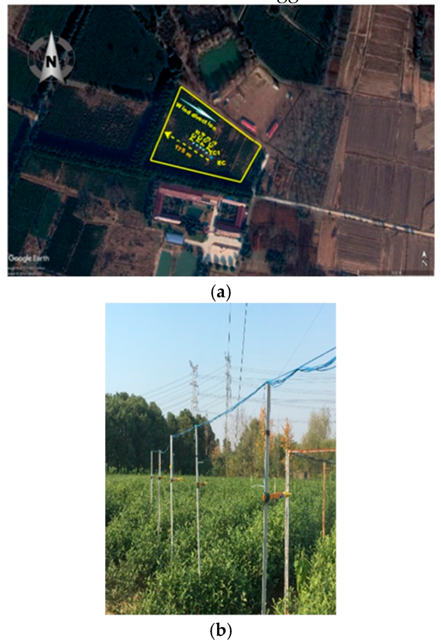
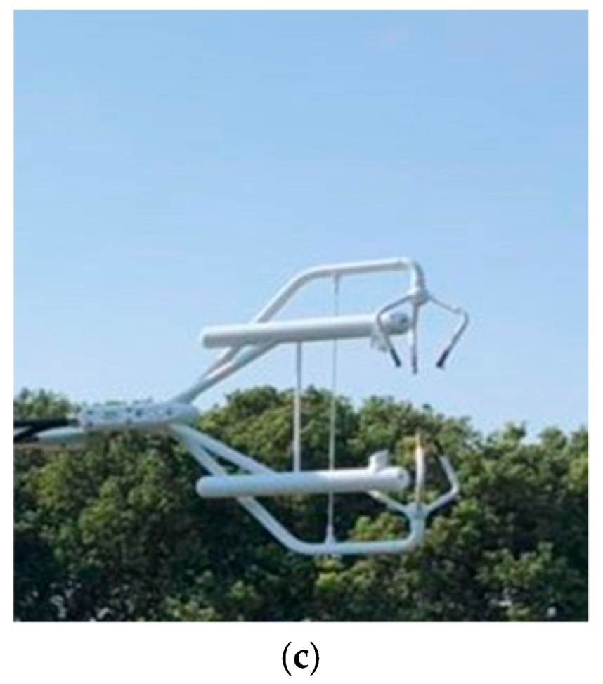
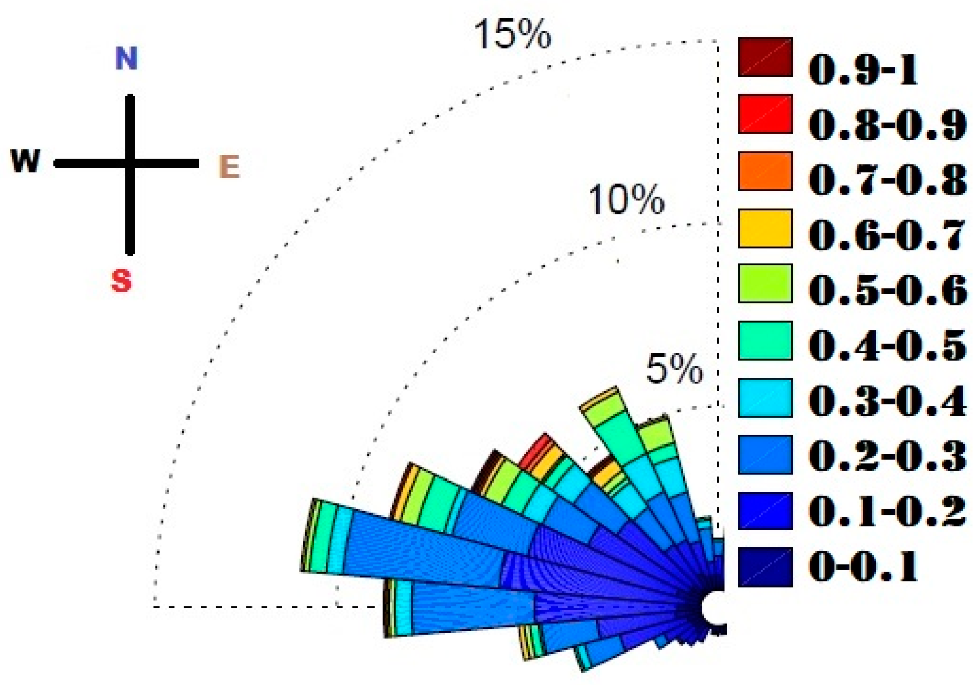
Eddy covariance (EC) measurements were performed approximately in the middle of the tea field at a position that allowed a fetch of about 175 m for the prevailing wind direction (Figure 2a). The EC system was installed at 2.3 m height, such that the available fetch in the prevailing wind direction, was approximately 100 times the measurement height above the zero-plane displacement (d) height according to the common rule of 1:100 height to fetch ratio [31]. The EC system consisted of two sensors (inset of Figure 2c): A three-dimensional sonic anemometer and an Open-path infrared gas analyzer, placed on a tower at the height of 2.3 m. This height is assumed to be above the roughness sublayer, estimated as 1.6 m, for the 0.8 m plant height. Sensors were oriented toward the dominant wind direction (West-North-West) (Figure 3) [32]. Raw data from the EC system was sampled at 10 Hz and stored in a CR3000 data logger. The measurements of sensible and latent heat flux by the EC system were processed using the Easyflux Software (Campbell Sci., USA) which deals with raw data filtering and corrections. Footprint analysis was performed to determine the 90% flux footprint to height ratio for the EC system and two different days were chosen for evaluation. See Table 3 for a list of sensors and their installation heights.
Other variables, including wind speed, wind direction (arctan v/u), air temperature, relative humidity (RH), rainfall, air pressure, soil temperature, and soil water content (ϴv), were sampled and half-hourly averages were recorded on a CR3000 data logger.
For the FV method, five unshielded type T fine-wire thermocouples (50 µm diameter) were used to measure the air temperature at a height of ~1.7 m above ground. The sensors were handled carefully during the experimental duration and were cleaned with Acetone solution (cleaning agent) after every two weeks. The five thermocouples were placed at different distances (TC1 = 170 m, TC2 = 165 m, TC3 = 160 m, TC4 = 155 m and TC5 = 150 m) from the field boundary (Figure 2a). A CR3000 data logger sampled thermocouples signals at 10 Hz.
Additional measurements were conducted for energy balance analysis. A net radiometer was installed at 2.3 m above the ground, towards the south, on the same pole with the EC system for measuring net radiation (Rn) (W m−2). Soil heat flux (G) was measured using two soil heat flux plates installed at a depth of 0.08 m in the soil and four soil temperature sensors, placed in the soil layer, two above each plate, at depths of 0.02 and 0.06 m respectively [33]. Half-hourly averages of measured variables (Rn, G, and soil temperature) were sampled and recorded on the CR3000 data logger. Dry batteries, charged by solar panels, were used as a power source.

3.3. Evaluation Criteria

The performance of the FV method was assessed separately for each thermocouple. RMSE was used to evaluate the accuracy of the estimations of the FV against the measurements of the EC method. In addition, regression analysis was performed to test how well the FV data fit the EC method. The following formulations were used for analysis: (a) Coefficient of determination (R2) Equation (8) [34], (b) the root mean square error (RMSE) Equation (9) [35] (c) Relative error (RE) Equation (10) [36]:
R 2 = ( i = 1 N ( X i X ¯ ) ( Y i Y ¯ ) ) 2 i = 1 N ( X i X ¯ ) 2 i = 1 N ( Y i Y ¯ ) 2
where X is the measurement of the EC system and Y is the estimation of the FV method.
RMSE = i = 1 N ( Y i X i ) 2 N ,  
where N is the number of half-hourly data points. The relative error (RE) was calculated as Equation (10):
RE   =   100   RMSE ( Y max Y min ) ,
where Ymax and Ymin are the maximum and minimum estimated values from the FV method respectively.

3.4. Possible Error Sources

Measurement errors may result either from sensors inaccuracy or from non-optimal conditions in the field measurements. Since all sensors used in this study were purchased just before the field campaign, they were under factory calibration, thus their inaccuracy was minimal. Furthermore, the fine-wire junctions of the thermocouples used for the FV analysis were frequently cleaned (Section 3.2.) to avoid performance deterioration, due to dirt accumulation. Another possible source of error is associated with the suitability of the specific field and atmospheric conditions for EC and FV flux measurements. To minimize this type of error the experiment was conducted in a homogeneous and horizontal tea field, and the sensors were positioned at a location and height that provided sufficient fetch for reliable flux measurements (see Section 4.1. below). Besides, the analysis was done only for data collected under unstable conditions, during daytime hours and rainless days. This minimized the number of data points with low turbulence conditions and assured that for most data points turbulence levels were satisfactory for reliable EC measurements. Hence it is assumed that errors of this type are at the same level as it is common in such field studies [5].

4. Results and Discussion

4.1. The Footprint of EC Flux Measurements

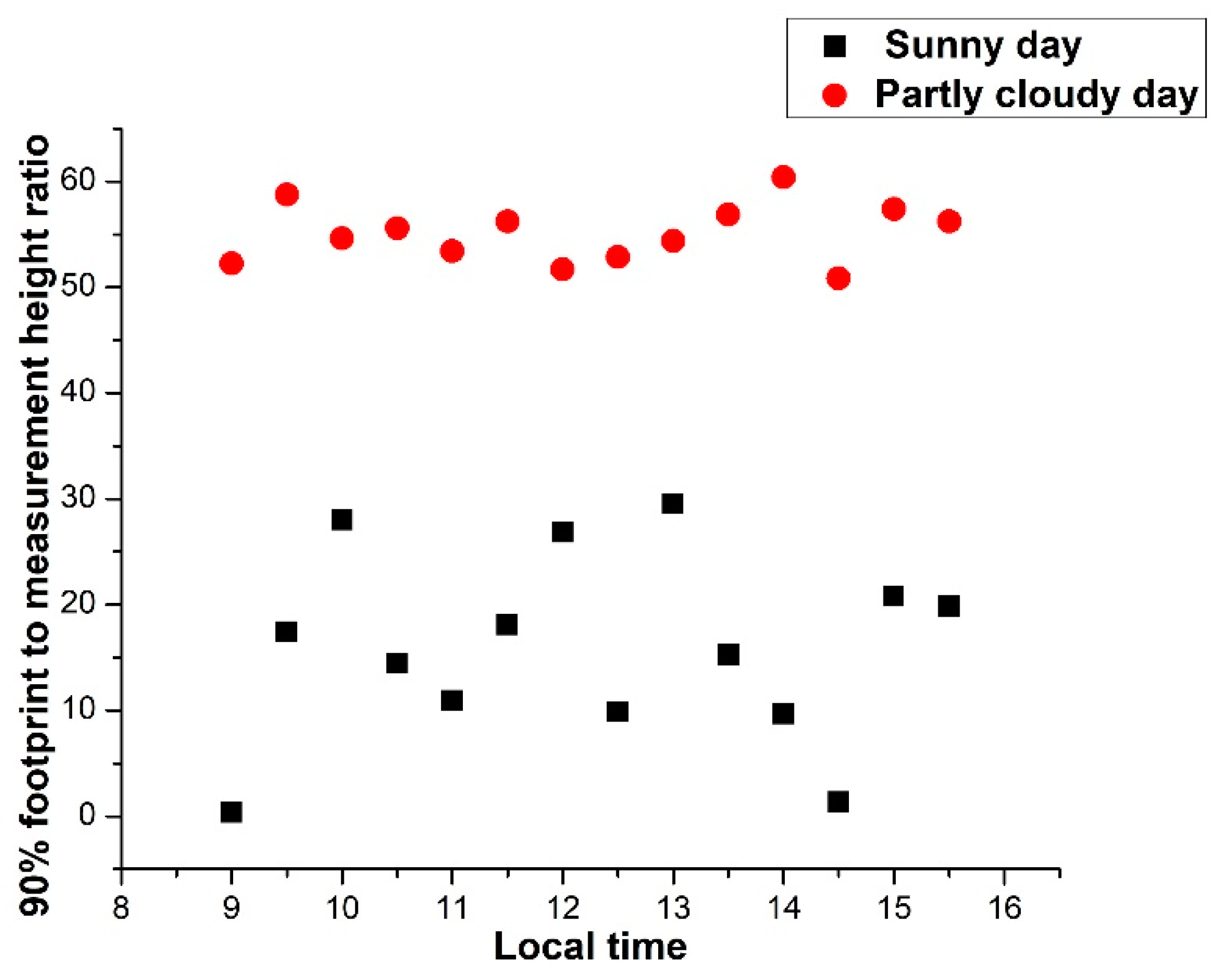
A footprint model was applied to analyze the relative contribution of the windward distance to surface fluxes measured by the EC system. The footprint model was estimated by Equations (5)–(7), which provide the ratio between 90% flux footprint and measurement height Equation (5). The analysis was performed mostly for the day time (unstable conditions) [27]. Two days with different climatic conditions were selected from the experimental duration: One (27/11/2018) partly cloudy and the other one (18/10/2018) a sunny day. Diurnal variation of footprint/height ratios for these two days are shown in Figure 4.
Results in (Figure 4) show that the ratio during the sunny day was in the range 0–30, significantly lower than the ratio determined during the partly cloudy day which ranged between 50 to 60. This difference is presumably because during the sunny day, the surface was warmer, and the boundary layer was more unstable than during the partly cloudy day. This larger instability resulted in a shorter 90% flux footprint during the sunny than the partly cloudy day. Besides, Figure 4 shows that in both days the ratio is smaller than the common 100:1 fetch/height ratio. This indicates that under the conditions of this experiment most of the flux measured by the EC system originated from within the tea field under study. Hence, the EC data is reliable and can be used as a reference to the FV method.

4.2. Energy Balance Closure Analysis

The analysis of EC data was done only for time intervals with a mean wind direction within 45° of the dominant wind direction [37]. The EC raw data were processed using the Easy-Flux DL, a data processing program by Campbell Scientific., USA. Raw data obtained during sensor fault or high precipitation days was discarded from all further analyses.
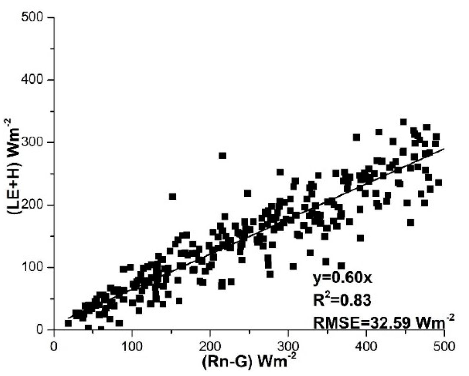
For the energy balance closure analysis, a linear regression was performed between the sum of half-hourly turbulent fluxes (LE+H) vs the available energy (Rn − G), as shown in (Figure 5). The linear regression is Equation (11):
L E   +   H   =   0.60 ( R n   G ) ,
where 0.60 is the closure slope (Figure 5). The reliability of the energy balance closure was justified with the slope of 0.60 and relatively high R2 = 0.83 which supports the reasonable quality of flux data measured by the EC and used for the further analysis against the FV estimations. Although the energy balance closure is low, this result is in good agreement with previous studies, as in most of the literature the slope is ranged between (0.55–0.99) for open fields [38,39]. These results support the use of HEC measured by the EC system to calibrate the similarity constant (CT) of the FV method using Equation (1).

4.3. Sensible Heat Flux Comparison

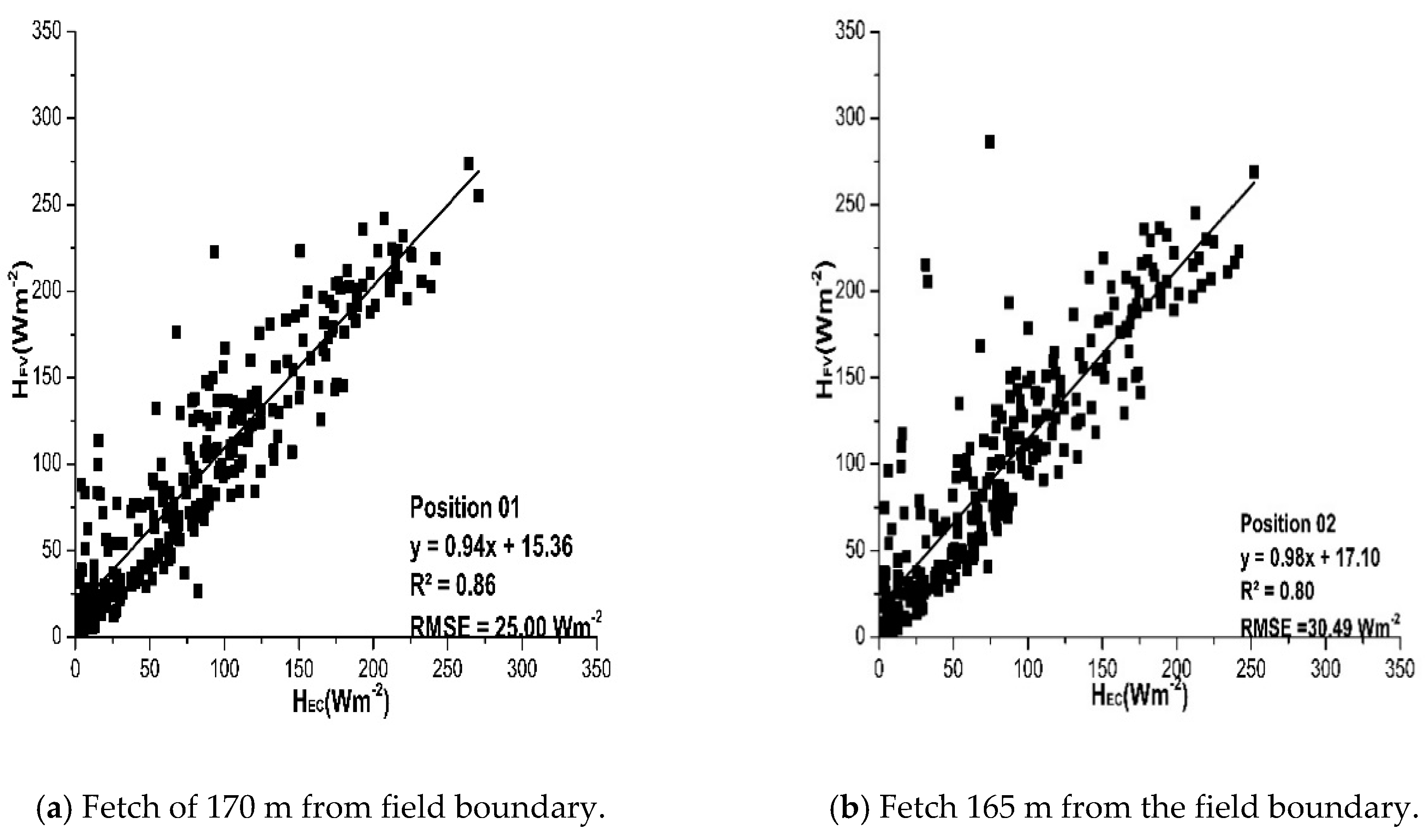
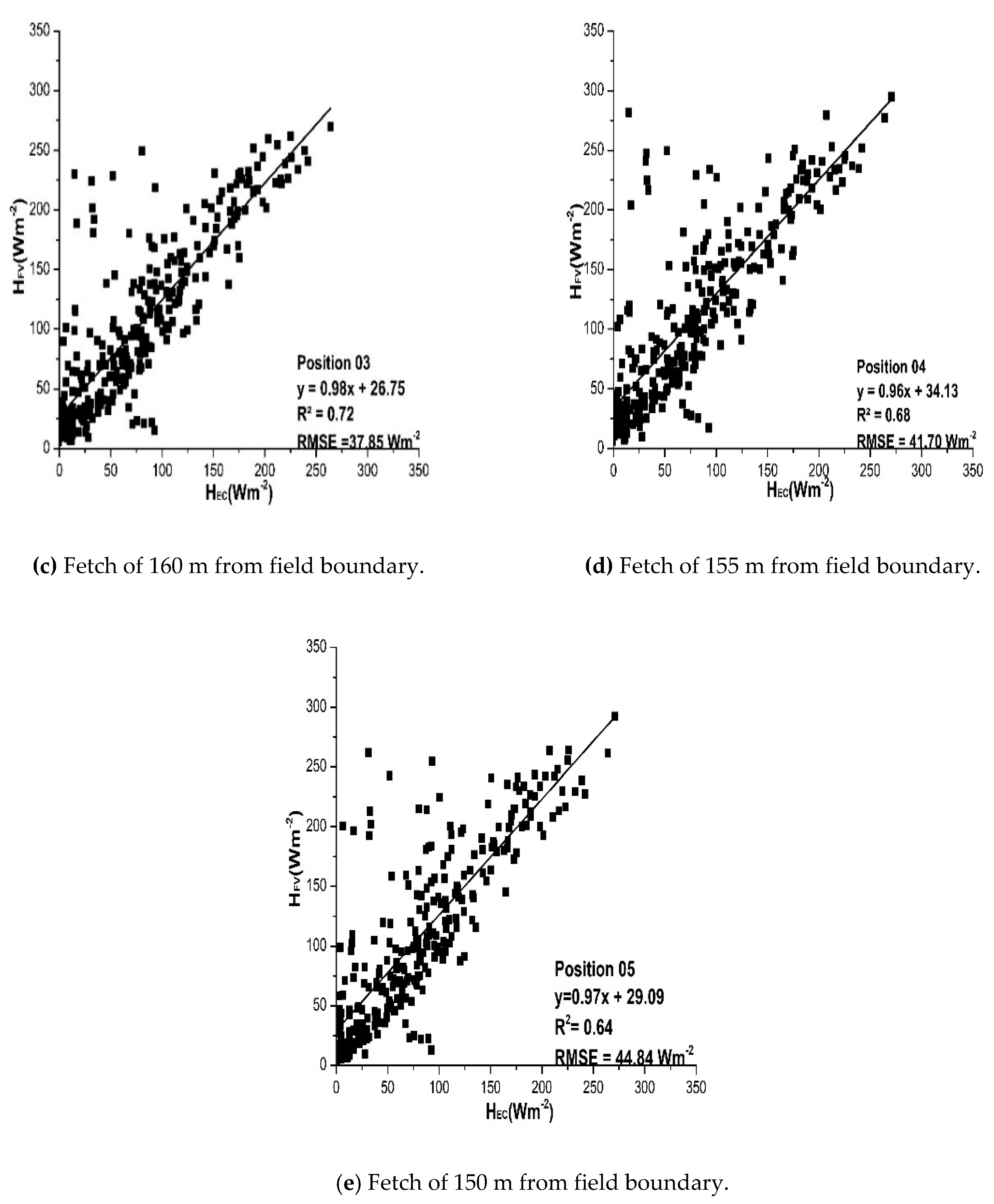
Results in Figure 6a−e show regressions between FV estimated and EC measured sensible heat flux, for five different thermocouple positions, under unstable conditions. The FV estimations are based on the similarity constant (CT) that was adjusted to give the best agreement between HFV and HEC for each position separately.
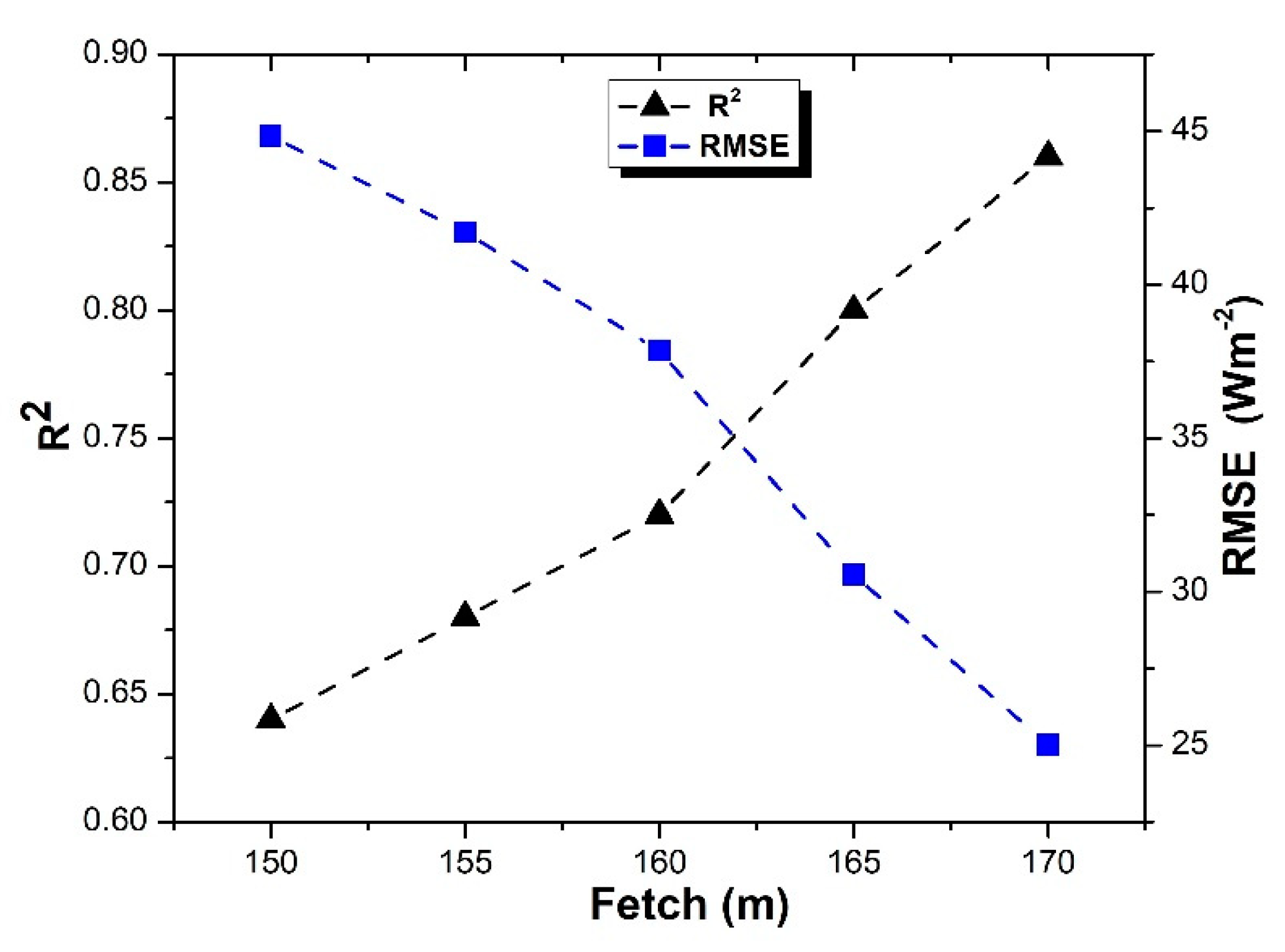
As shown in Figure 6a, very good agreement was observed between the 30-min estimations of HFV and HEC at 170 m from the field edge, with a slope of 0.94, a relatively high R2 = 0.86, low RMSE = 25 Wm−2 and relative error RE = 9.25%. All estimations at the other positions were also in good agreement with the measurements of the EC method, with R2 always larger than 0.6. Some data points, especially in Figure 6b–e show a relatively high estimation of HFV as compared to HEC. The analysis showed that this occurred mainly in the later part of the day, from 15:00 to 16:00. The parameters of regressions between HFV and HEC flux estimates at the five positions are presented in Table 4 and plotted in Figure 7. Figure 7 clearly shows that R2 increases, whereas RMSE decreases with increasing fetch. Hence, a larger fetch provides a better agreement between FV and EC sensible heat flux. This is presumably because with a larger fetch the surface layer becomes more developed and the FV approach, which is based on MOST, is more valid.
Another important parameter in the FV analysis is the similarity constant (CT), estimated from the regression analysis between H measurements of the EC system and that estimated by the FV method using Equation (1). In the present study, the estimated CT was ranging between 2.2 and 2.4 (Table 4) with an average value of 2.3 [40]. Overall, it was observed from the study that the similarity constant was independent of the fetch.
This is the first study that analyzed the effect of variable fetch on the performance of the FV method under open field conditions. The results of this study, regarding the variability of R2 and CT with fetch (Table 4) are qualitatively similar to those by Tanny et al [14] who studied the FV method in a screenhouse in which pepper was grown. In both studies, R2 of the regression between HEC and HFV increased with fetch, indicating the spatial development process of the surface layer and the increasing validity of MOST with distance. The similarity constant obtained in the screenhouse by Tanny et al. [14] was about 3.8, significantly larger than the value obtained here of 2.3. This could be explained by the presence of the screened roof in Tanny et al.’s experiment, which presumably inhibited the development of the turbulence as compared to the open field studied here [14].

4.4. Latent Heat Flux Estimation

The latent heat flux (LE) was estimated as a residual of the energy balance Equation (12):
L E F V = 0.60 ( R n   G )     H F V .
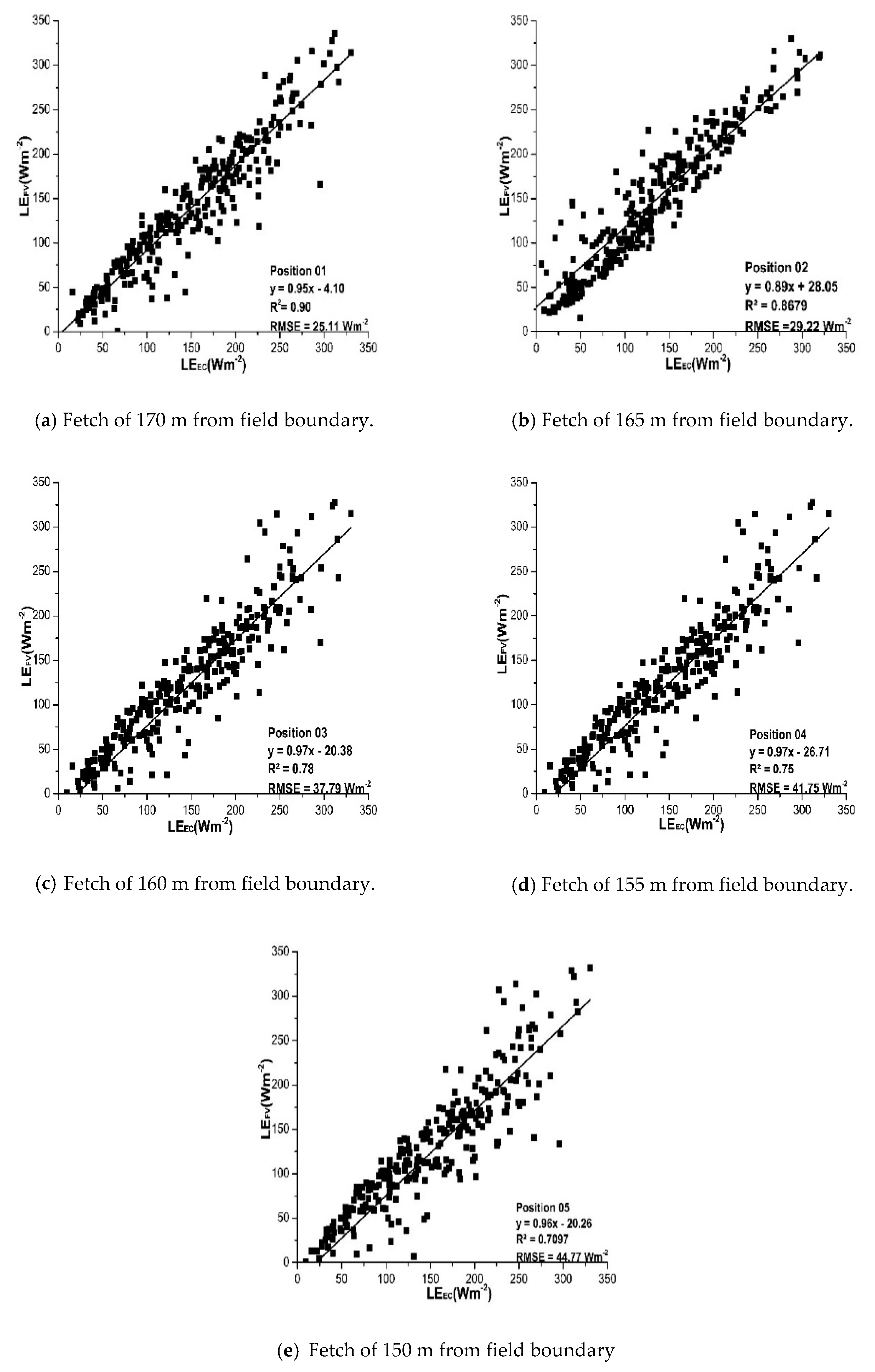
The regression statistics were performed separately for each thermocouple along the fetch. Since the FV data was analyzed only under unstable conditions, and these prevail mostly during the daytime, only daytime values of the latent energy flux were analyzed. The regressions between the LEFV and measured LEEC, are presented in (Figure 8a–e).
Statistical analysis of the results presented in Table 5, showed that R2 varied from TC1 to TC5 along the fetch. The LEFV gave a good estimate of LEEC for all thermocouples and all the slopes were close to unity with RMSE always less than 45 Wm−2. The FV latent heat flux at TC1 which was closest to the EC system and had the longest fetch yielded best results with a slope 0.95, lowest RMSE of 25.11 Wm−2, lowest RE of 4.73 %, and largest R2 = 0.90, as compared to all other thermocouples. The performance of the LEFV, as indicated by RMSE, was improved as position changed and became closer to the EC system and with longer fetch. The overall estimates of LEFV, at all positions, were in good agreement with the measurements of the EC system.
The independence of the FV performance on the fetch observed here implies that the method could be reliable also under conditions of smaller fetch than that realized here (although this was not examined in the present study). A recent study by Haymann et al. (2019) has demonstrated a similar observation regarding another micrometeorological method, the Surface Renewal (SR) [41]. The possibility of reliable LE estimations under limited fetch might be applicable for measurements in small agricultural fields or in agricultural field trials where small plots with different treatments are studied. It provides a significant advantage of the FV method over the EC where large fetch is mandatory.

5. Conclusions and Outlook

In this study, the effect of variable fetch on the performance of the FV method for the estimation of surface fluxes of H and LE in the open field was studied for the first time. The results showed that the FV method was reliable for the estimation of H and provided an accurate estimation of LE. The similarity constant (CT), estimated from the regression analysis between the H estimates of the FV and the measurements by the EC method, changed along the fetch, but a consistent trend was not observed, and it was concluded that the CT has a mean value of 2.3, and is independent of the fetch. The regression between the HFV and HEC for the TC1 which is very close to the EC system and far from the field edge provided higher R2 = 0.86 and lower RMSE = 25 Wm−2 relative to the other thermocouples. In summary, the FV method proved to be a reliable method for the monitoring of surface fluxes at low cost as compared to the EC method.
The FV method is an attractive candidate to be used by growers for day-to-day estimates of LE as an aid in irrigation management. However, two aspects should be examined before it can be considered for routine application. First, it is obvious that farmers will not operate an EC system for FV calibration. Hence, a question of interest is how robust is the similarity constant obtained in this study for other tea plantations. This requires additional field campaigns in other tea plantations. The second aspect is the long-term performance of the fine-wire thermocouples. In this study, the miniature thermocouple junction was frequently cleaned to avoid dirt accumulation. However, it is not clear yet how long such a junction can provide reliable data and whether it should be replaced periodically. To resolve this question, a long-term study should be performed where possible temporal variations of sensor performance would be addressed. Another benefit of such a long-term study would be the examination of the FV performance under various weather conditions, which is missing from this study that was conducted during a relatively limited period of time.

Author Contributions

N.A.B. drafted the manuscript, executed the statistical analysis, interpreted the results, and wrote the manuscript. H.Y. supervised all the experimental setup and reviewed some results. J.T. reviewed the manuscript, interpreted results, commented on the manuscript and participated in revision. A.S. and M.W.A. participated in data analysis.

Funding

The authors are grateful to the financial support by Jiangsu Agriculture Science and Technology Innovation Fund (CX (16)1045), the Key R&D programs of Jiangsu Province and Zhenjiang (BE2016354 and NY2018007), Six Talent Peaks Program of Jiangsu Province (2015-ZBZZ-021) and Priority Academic Program Development of Jiangsu Higher Education Institutions.

Conflicts of Interest

The authors declare no conflict of interest.

References

  1. Jarmain, C.S.C.; Everson, M.J.; Savage, M.G.; Mengistu, A.D.; Clulow, S.W.; Gush, M.B. Refining Tools for Evaporation Monitoring in Support of Water Resources Management; Water Research Commission: Pretoria, South Africa, 2009. [Google Scholar]
  2. Allen, R.G.; Luis, S.; Pereira, D.R.; Smith, M. Crop Evapotranspiration-Guidelines for Computing Crop Water Requirements-FAO Irrigation and Drainage Paper; FAO: Rome, Italy, 1998; Volume 300. [Google Scholar]
  3. Saigusa, N.; Yamamoto, S.; Hirata, R.; Ohtani, Y.; Ide, R.; Asanuma, J.; Gamo, M.; Hirano, T.; Kondo, H.; Kosugi, Y.; et al. Temporal and spatial variations in the seasonal patterns of CO2 flux in boreal, temperate, and tropical forests in East Asia. Agric. For. Meteorol. 2008, 148, 700–713. [Google Scholar] [CrossRef]
  4. Hollinger, D.Y.; Aber, J.; Dail, B.; Davidson, E.A.; Goltz, S.M.; Hughes, H.; Leclerc, M.Y.; Lee, J.T.; Richardson, A.D.; Rodrigues, C.; et al. Spatial and temporal variability in forest–atmosphere CO2 exchange. Glob. Chang. Biol. 2004, 10, 1689–1706. [Google Scholar] [CrossRef]
  5. Aubinet, M.; Timo, V.; Papale, D. (Eds.) Eddy Covariance: A Practical Guide to Measurement and Data Analysis; Springer Science and Business Media: Berlin, Germany, 2012. [Google Scholar]
  6. Hu, Y.; Buttar, N.A.; Tanny, J.; Snyder, R.L.; Savage, M.J.; Lakhiar, I.A. “Surface Renewal Application for Estimating Evapotranspiration: A Review”. Adv. Meteorol. 2018, 2018, 1690714. [Google Scholar] [CrossRef]
  7. Wesely, M.L.; Thurtell, G.W.; Tanner, C.B. Eddy correlation measurements of sensible heat flux near the earth’s surface. J. Appl. Meteorol. 1970, 9, 45–50. [Google Scholar] [CrossRef]
  8. Tillman, J.E. The indirect determination of stability, heat and momentum fluxes in the atmospheric boundary layer from simple scalar variables during dry unstable conditions. J. Appl. Meteorol. 1972, 11, 783–792. [Google Scholar] [CrossRef]
  9. Wesson, K.H.; Gabriel, K.; Chun-Ta, L. Sensible heat flux estimation by flux variance and half-order time derivative methods. Water Resour. Res. 2001, 37, 2333–2343. [Google Scholar] [CrossRef] [Green Version]
  10. Weaver, H.L. Temperature and humidity flux-variance relations determined by one-dimensional eddy correlation. Bound. Layer Meteorol. 1990, 53, 77–91. [Google Scholar] [CrossRef]
  11. Lloyd, C.R.; Culf, A.D.; Dolman, A.J.; Gash, J.H.C. Estimates of sensible heat flux from observations of temperature fluctuations. Bound. Layer Meteorol. 1991, 57, 311–322. [Google Scholar] [CrossRef]
  12. Albertson, J.D.; Marc, B.; Parlange, G.G.; Katul, C.-R.C.; Stricker, H.; Scott, T. Sensible heat flux from arid regions: A simple flux-variance method. Water Resources Res. 1995, 31, 969–973. [Google Scholar] [CrossRef]
  13. Ali Buttar, N.; Hu, Y.; Zhang, C.; Josef, T.; Ikram, U.; Muhammad, A. Height effect of air temperature measurement on sensible heat flux estimation using flux variance method. Pak. J. Agric. Sci. 2019, 56, 793–800. [Google Scholar]
  14. Tanny, J.O.; Achiman, Y.; Mazliach, V.; Lukyanov, S.C.; Cohen, T. The effect of variable fetch on flux-variance estimates of sensible and latent heat fluxes in a pepper screenhouse. In Proceedings of the International Symposium on Sensing Plant. Water Status-Methods and Applications in Horticultural Science, Potsdam, Germany, 6 October 2016; Volume 1197, pp. 109–116. [Google Scholar]
  15. Ahiman, O.; Mekhmandarov, Y.; Pirkner, M.; Tanny, Y. Application of the Flux-Variance Technique for Evapotranspiration Estimates in Three Types of Agricultural Structures. Int. J. Agron. 2018, 2018, 7935140. [Google Scholar] [CrossRef]
  16. Choi, T.; Hong, J.; Kim, J.; Lee, H.; Asanuma, J.; Ishikawa, H.; Tsukamoto, O.; Zhiqiu, G.; Ma, Y.; Ueno, K.; et al. Turbulent exchange of heat, water vapor, and momentum over a Tibetan prairie by eddy covariance and flux variance measurements. J. Geophys. Res. Atmos. 2004, 109, doi. [Google Scholar] [CrossRef]
  17. Sugita, M.; Noriaki, K. Surface and mixed-layer variance methods to estimate regional sensible heat flux at the surface. Bound. Layer Meteorol. 2003, 106, 117–145. [Google Scholar] [CrossRef]
  18. De Bruin, H.A.R.; Hartogensis, O.K. Variance method to determine turbulent fluxes of momentum and sensible heat in the stable atmospheric surface layer. Bound. Layer Meteorol. 2005, 116, 385–392. [Google Scholar] [CrossRef]
  19. Stull, R.B. Similarity Theory. In An Introduction to Boundary Layer Meteorology; Springer: Dordrecht The Netherlands, 1988; pp. 347–404. [Google Scholar]
  20. Stull, R.B. Transilient turbulence theory. Part I: The concept of eddy-mixing across finite distances. J. Atmos. Sci. 1984, 41, 3351–3367. [Google Scholar] [CrossRef]
  21. Garratt, J.R. The atmospheric boundary layer. Earth-Sci. Rev. 1994, 37, 89–134. [Google Scholar] [CrossRef]
  22. Deardorf, J.W. Observed characteristics of the outer layer. AMS course on the planetary boundary layer. Boulder, Colorado, 1983; (unpublished manuscript). [Google Scholar]
  23. Detering, H.W.; Etling, D. Application of the E-ε turbulence model to the atmospheric boundary layer. Bound. Layer Meteorol. 1985, 33, 113–133. [Google Scholar] [CrossRef]
  24. Kljun, N.P.; Calanca, M.W.; Rotach, S.; Schmid, H.P. A simple two-dimensional parameterisation for Flux Footprint Prediction (FFP). Geosci. Model. Develop. 2015, 8, 3695–3713. [Google Scholar] [CrossRef] [Green Version]
  25. Gash, J.H.C. A note on estimating the effect of a limited fetch on micrometeorological evaporation measurements. Bound. Layer Meteorol. 1986, 35, 409–4134. [Google Scholar] [CrossRef]
  26. Savage, M.J.; Everson, C.S.; Rawstorne Metelerkamp, B. Evaporation measurement above vegetated surfaces using micrometeorological techniques. Pretoria. Water Res. Comm. 1997. [Google Scholar]
  27. Hsieh, C.-I.; Mei-Chun, L.; Yue-Joe, H.; Tsang-Jung, C. Estimation of sensible heat, water vapor, and CO2 fluxes using the flux-variance method. Int. J. Biometeorol. 2008, 52, 521–533. [Google Scholar] [CrossRef]
  28. Savage, M.J.; Everson, C.S.; Odhiambo, G.O.; Mengistu, M.G.; Jarmain, C. Theory and Practice of Evaporation Measurement, with Spatial Focus on SLS as an Operational Tool for the Estimation of Spatially-Averaged Evaporation; Report No. 1335/1/04; Water Research Commission: Pretoria, South Africa, 2004; p. 204. ISBN 1−77005−247−X. [Google Scholar]
  29. Hsieh, C.-I.; Gabriel, K.; Tzewen, C. An approximate analytical model for footprint estimation of scalar fluxes in thermally stratified atmospheric flows. Adv. Water Res. 2000, 23, 765–772. [Google Scholar] [CrossRef]
  30. Hu, Y.; Zhu, X.; Zhao, M.; Richard, L.; Snyder, L.; Li, P. Operation effects of wind machines for frost protection of tea trees on different time scales. Nongye Jixie Xuebao Transact. Chin. Soc. Agric. Mach. 2013, 44, 252–257. [Google Scholar]
  31. Allen, R.G.; Pereira, L.S.; Howell, T.A.; Jensen, M.E. Evapotranspiration information reporting: I. Factors governing measurement accuracy. Agric. Water Manag. 2011, 98, 899–920. [Google Scholar] [CrossRef] [Green Version]
  32. Foken, T.; Napo, C.J. Micrometeorology; Springer: Berlin, Germany, 2008; Volume 2. [Google Scholar]
  33. Tanner, C.B.; Pelton, W.L. Potential evapotranspiration estimates by the approximate energy balance method of Penman. J. Geophys. Res. 1960, 65, 3391–3413. [Google Scholar] [CrossRef]
  34. Cameron, A.C.; Windmeijer, F.A.G. An R-squared measure of goodness of fit for some common nonlinear regression models. J. Econom. 1997, 77, 329–342. [Google Scholar] [CrossRef]
  35. Willmott, C.J. Some comments on the evaluation of model performance. Bull. Am. Meteorol. Soc. 1982, 63, 1309–1313. [Google Scholar] [CrossRef]
  36. Willmott, C.J.; Matsuura, K. Advantages of the mean absolute error (MAE) over the root mean square error (RMSE) in assessing average model performance. Climate Res. 2005, 30, 79–82. [Google Scholar] [CrossRef]
  37. Wilson, K.; Goldstein, A.; Falge, E.; Aubinet, M.; Baldocchi, D.; Berbigier, P.; Bernhofer, C.; Ceulemans, R.; Dolman, H.; Field, C.; et al. Energy balance closure at FLUXNET sites. Agric. For. Meteorol. 2002, 113, 223–243. [Google Scholar] [CrossRef] [Green Version]
  38. Kordova-Biezuner, L.; Mahrer, I.; Schwartz, C. Estimation of actual evapotranspiration from vineyard by utilizing eddy correlation method. In Proceedings of the III International Symposium on Irrigation of Horticultural Crops, Lleida, Spain, 8 June 1999; Volume 537, pp. 167–175. [Google Scholar]
  39. Testi, L.; Villalobos, F.J.; Orgaz, F. Evapotranspiration of a young irrigated olive orchard in southern Spain. Agric. For. Meteorol. 2004, 121, 1–18. [Google Scholar] [CrossRef]
  40. Wyngaard, J.C.; Coté, O.R.; Izumi, Y. Local free convection, similarity, and the budgets of shear stress and heat flux. J. Atmos. Sci. 1971, 28, 1171–1182. [Google Scholar] [CrossRef]
  41. Haymann, N.; Lukyanov, V.; Tanny, J. Effects of variable fetch and footprint on surface renewal measurements of sensible and latent heat fluxes in cotton. Agric. For. Meteorol. 2019, 268, 63–73. [Google Scholar] [CrossRef]
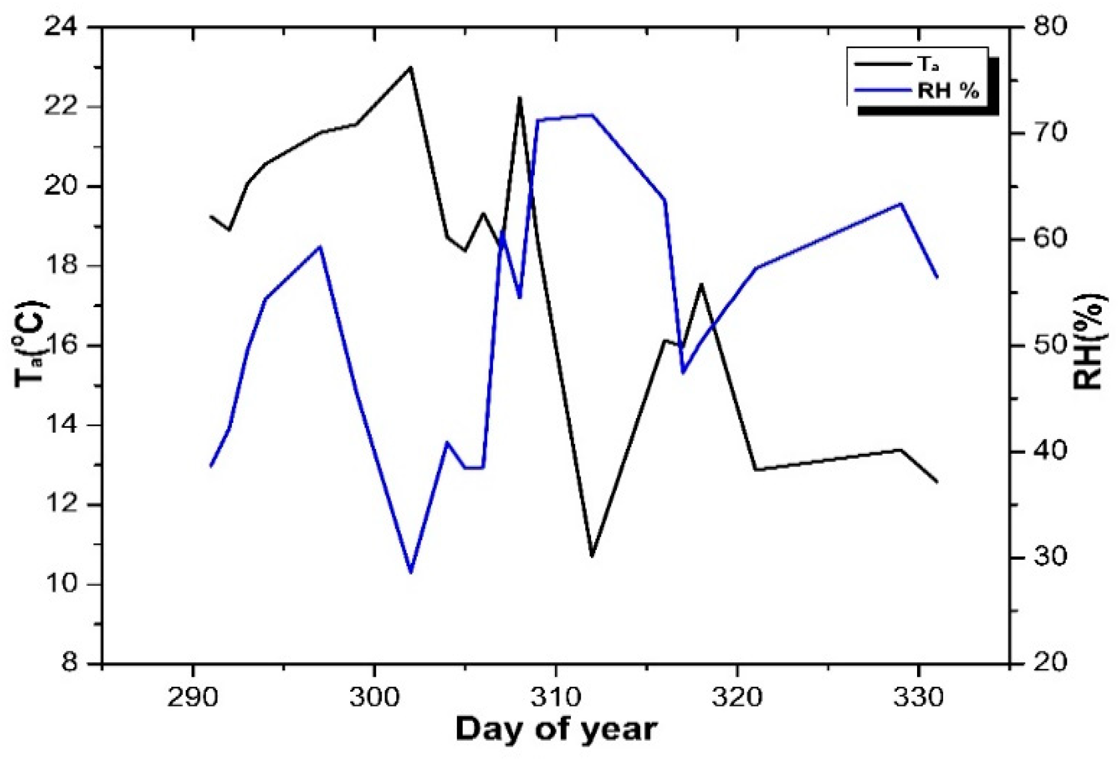
Figure 1. Mean daily values of air temperature and relative humidity for the whole experimental period.
Atmosphere 10 00299 g001
Figure 2. The experimental setup (a) Schematic top view of the tea field with thermocouples positions (TC1…TC5) and EC system (Pic from google earth). (b) Photo of the TC sensors distributed in the tea field along the prevailing wind direction. (c) The EC system (Campbell Scientific, USA).
Atmosphere 10 00299 g002aAtmosphere 10 00299 g002b
Figure 3. The wind rose presentation of wind direction and wind speed (m s−1) during the experiment period of Sept–Nov 2018. The prevailing wind direction of West-North-West is clearly observed.
Atmosphere 10 00299 g003
Figure 4. Variation of half-hourly 90% footprint to measurement height ratio Equation (5) for two days one partly cloudy (27/11/2018) and the other with a clear sky (sunny day) (18/10/2018) [28].
Atmosphere 10 00299 g004
Figure 5. Linear regression between the components of the energy balance closure based on the EC flux measurements.
Atmosphere 10 00299 g005
Figure 6. (a) Fetch of 170 m from field boundary; (b) Fetch 165 m from the field boundary; (c) Fetch of 160 m from field boundary; (d) Fetch of 155 m from field boundary; (e) Fetch of 150 m from field boundary. Regression analysis between the estimated HFV and measured HEC at five different positions along the fetch.
Atmosphere 10 00299 g006aAtmosphere 10 00299 g006b
Figure 7. Variation of R2 and RMSE for HFV vs HEC along fetch.
Atmosphere 10 00299 g007
Figure 8. (a) Fetch of 170 m from field boundary; (b) Fetch of 165 m from field boundary; (c) Fetch of 160 m from field boundary; (d) Fetch of 155 m from field boundary; (e) Fetch of 150 m from field boundary. Half-hourly LEFV derived by using Equation (12) plotted against LEEC for unstable conditions during Sep–Nov 2018.
Atmosphere 10 00299 g008
Table 1. Stability condition with respect to Obukhov length [22,23].
Stability ConditionObukhov Length (L)
Stable0 < L < 200
Unstable−200 < L < 0
Neutral|L| > 200
Table 2. Similarity constants (D and P) for different stability conditions [29].
DPStability Condition
0.280.59Unstable
0.971Natural
2.441.33Stable
Table 3. List of sensors, units, measurement height and equipment used in the experiment.
NotationUnitsHeight (m)Equipment
3D-Wind velocity, Sonic temperature u, v, w, Tsm s−1, °C2.3CSAT3, Sonic anemometer, Campbell Scientific, USA.
H2O and CO2 concentrations-µmol m−32.3EC150, Campbell Scientific., USA.
Soil temperatureTsoil°C0.02 and 0.06 (Depth)TCAV-L, Campbell Scientific, USA.
Air temperature for FV analysisTa°C1.7Fine-wire thermocouple, COCO-002, Omega, Eng., UK.
Relative humidityRH%2.1HC2S3-L, Campbell Scientific., USA.
Soil heat fluxGW m−20.08HFP01, Hukseflux plate sensor.
Net radiationRnW m−22.3CNR4-L, KIPP and ZENON.
Liquid precipitation-mm2.1TE525MM, Campbell Scientific Inc., USA.
Soil water contentϴvm3m−30.04 (Depth)CS655, Campbell Scientific Inc., USA.
Table 4. Statistical parameters of the regressions between HEC and HFV at the different positions: R2, the similarity constant CT, RMSE, RE, and slope. n is the number of data points in each regression. Fetch is the distance from the field edge for the dominant wind direction.
StatisticsHFV
SensorsTC1TC2TC3TC4TC5
Fetch (m)170165160155150
R20.860.800.720.680.64
CT2.32.42.32.22.3
RMSE (Wm−2)25.0030.5537.8541.7044.84
RE (%)9.2510.7414.3314.4412.57
Slope0.940.980.980.960.97
n291289294291293
Table 5. Regression statistics of half-hourly LEFV vs LEEC as indicated by R2, RMSE, RE and the slope of linear regression.
StatisticsLEFV
SensorsTC1TC2TC3TC4TC5
Fetch (m)170165160155150
R20.900.870.780.750.71
RMSE (Wm−2)25.1129.2237.7941.7444.77
RE (%)4.735.967.527.787.03
Slope0.950.870.970.970.96
n291289294291293