1. Introduction
Actual Evapotranspiration (AET), which is the water lost to the atmosphere from the land surface [
1], is a crucial component of the terrestrial water cycle and energy balance [
2,
3]. In addition, accurate AET information at a regional scale is critical for quantitative understanding of land-atmosphere interactions and providing valuable means to efficiently use water resources [
4,
5]. However, it is difficult to measure AET through point observation in remote mountain regions, such as the Tibetan Plateau (TP), which also has harsh climate conditions. The TP, with an average elevation of more than 4000 m above sea level, is often called the ‘Third Pole’ because of excessive amounts of snow and ice existing, especially for mountainous regions. The large heat sink created during the spring and summer has a profound impact on the mid-troposphere [
6,
7]. The thermal forcing effectively enhances the Asian monsoon and modulates its variability [
8]. In addition, for the water cycle, the TP contains the headwaters of major rivers in Asia and is often referred to as the ‘Asian Water Tower’ [
9].
Several eddy-flux towers have been set up in the TP [
10], but they cannot provide sufficient or accurate estimations of regional AET over a heterogeneous area. With rapid development of remote sensing technology, regional and meso-scale patterns of the characteristics of land surface parameters used for AET estimation can be mapped efficiently with satellite data [
11]. Therefore, several satellite-based AET approaches are applicable for determining AET at different scales, which include simplified empirical regressions and physically based surface energy balance (SEB) models [
12,
13,
14,
15,
16]. The empirical methods can be established based on in situ measurements of AET and related hydrometeorological parameters for different homogeneous regions. This kind of method has some advantages due to its simplicity. The empirical models are more accurate under the in-situ conditions it is based on. If these conditions are fairly homogenous over large scales, empirical models can be accurate enough. For heterogeneous regions, empirical models have their limitations. The physically-based models use meteorological parameters and land surface parameters retrieved from satellite images as model inputs. The calculation for these models include complex solution of the turbulent heat fluxes. However, these models have the ability to estimate meso-scale, regional scale, and even global scale AET with reasonable accuracy. They have other advantages, such as low cost, continuous monitoring, and clear physical mechanisms involved. The physically-based surface energy balance models have been widely used to estimate AET with the aid of remote sensing techniques [
14,
15,
17,
18].
Although researches on the estimation of AET have become available for various applications [
11,
19], most of them only focus on the regional scale or the global scale. AET is still difficult to calculate accurately because of the heterogeneous landscape and the large number of controlling factors involved. Studies on the estimation of AET at a basin scale over the TP are rather scarce. Furthermore, in recent inter-comparisons of global AET estimation results, large model uncertainties were observed [
20]. First, these uncertainties come from different models and approaches for calculating AET. Second, for a heterogeneous land surface like the TP, the roughness length for heat transfer in a model can vary with geometric and environmental variables by several orders of magnitude. Large uncertainties are caused by estimating evaporation for different land surface types [
20]. Third, some of the model input forcing parameters need improvement. For example, most of the previous models used vegetation indices processed by the maximum value compositing (MVC) method while the effects of cloud cover were not removed completely [
21].
Since basin-scale AET data are crucial to close the water cycle, more attention should be paid to local basin scale studies such as the Nagqu river basin over the TP. The motivation for the current study is that regional AET data over the TP with reasonable accuracy are still needed. This study aims to test the feasibility of the surface energy balance system (SEBS) model to derive the AET at a local basin scale. As input parameters for AET calculations, broadband albedo was parameterized with a new formula. Normalized difference vegetation index (NDVI) was reconstructed by cloud removal before being added to the model.
2. Materials
Taking the quality and continuity of in-situ measurements into account, this study mainly focuses on the year 2003. Daily meteorological data, surface meteorological forcing data, 10-day composite SPOT Vegetation (VGT) data, and daily Moderate Resolution Imaging Spectroradiometer (MODIS) data were used as an input for 10-day mean AET calculations.
2.1. Study Area
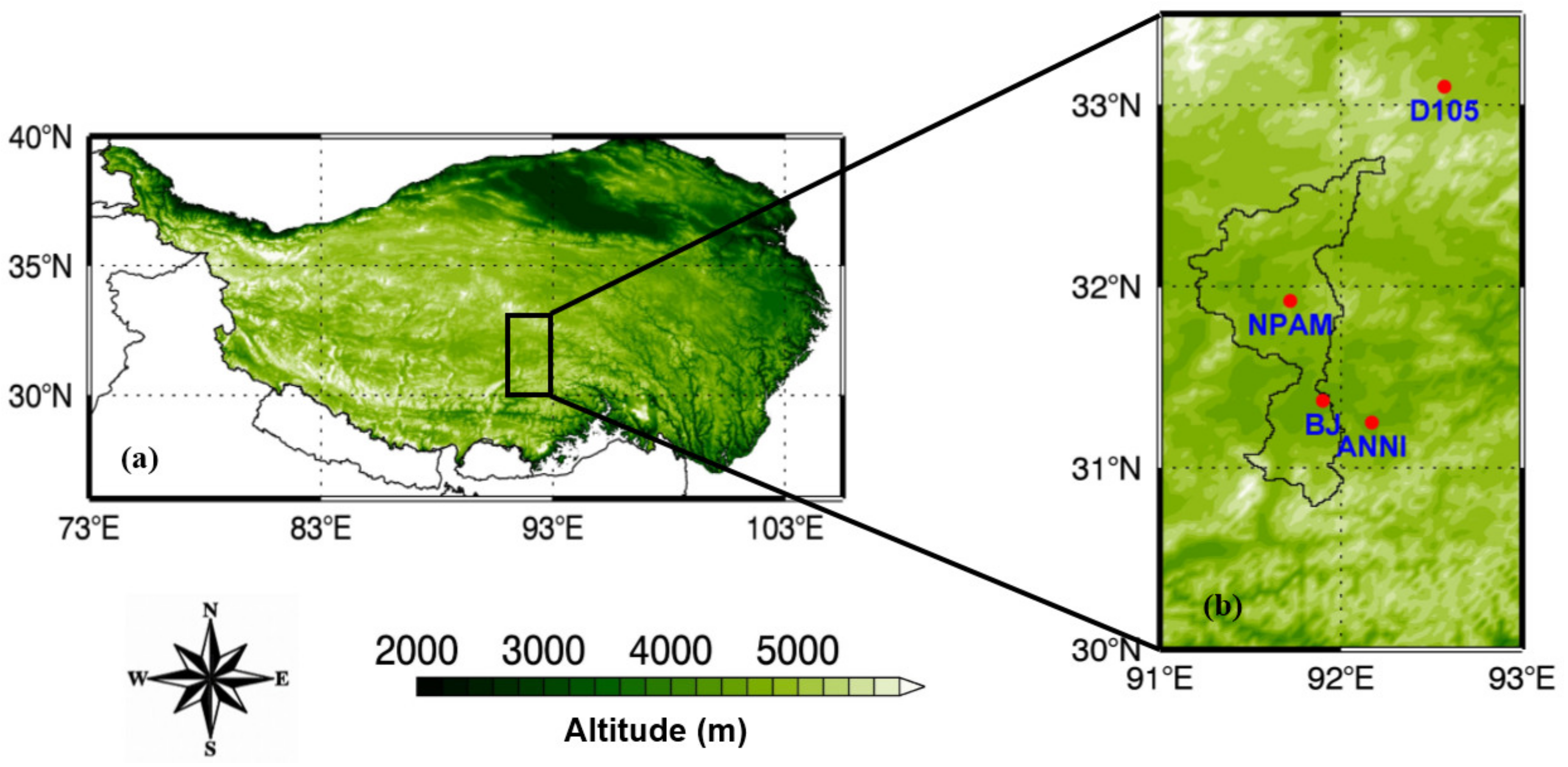
The Nagqu river basin, which is located in the southern part of the TP, China, has a size of about 8749 km
2 and a mean elevation of more than 4808 m above sea level (
Figure 1). It is located between the Tanggula Mountains and the Nyainqentanglha Mountains [
22]. The Nagqu river basin is part of the Nu River system. Gentle hills and mountains are scattered throughout the entire basin terrain. The dominant vegetation type is meadow. Strong solar radiation and low air temperature are two characteristic climate conditions for the study area. The annual precipitation is about 430.2 mm with monthly sums ranging from 3.2 mm (January) to 103.1 mm (July). A clear demarcation between the dry and wet season is identified due to the influence of the Asian monsoon. Approximately 80% of the total precipitation falls during the wet season (from June to August).
2.2. Satellite Data
The input satellite data are shown in
Table 1. The datasets include: (1) 1-km MODIS land surface temperature (LST) data (MOD11A1), (2) 1-km VGT NDVI, (3) 1-km VGT narrowband albedo, (4) 30-m ASTER digital elevation model (DEM), (5)
MODIS aerosol optical depth (AOD) (MOD08D3), and (6) 1-km MODIS land cover type (LCT) data (MOD12Q1). Since clouds are always occurring in the satellite images, we only choose images taken with total cloud cover of less than 40% in this study. With ancillary information from MOD06_L2, images with cloud cover of more than 40% were excluded. To maintain consistency in spatial and temporal resolution, all satellite data were preprocessed by temporal-spatial matching. The spatial resolution was aggregated into 1 km cells using a nearest neighbor interpolation method and the daily temporal resolution was averaged into 10-day intervals.
2.3. In Situ Data and Surface Forcing Data
Taking data continuity and quality into account, the Northern Portable Automated Meso-net (NPAM) and Bu Jiao (BJ) stations in the Nagqu river basin, together with the D105 and ANNI stations around the study area were used. The observational data for 2003 from the Coordinated Enhanced Observing Period Asia–Australia Monsoon Project on the Tibetan Plateau (CAMP/Tibet) were used as inputs for the combinatory method (CM). The in situ meteorological data included hourly multiple-layer air temperature, relative humidity, wind speed, soil heat flux, air pressure, and soil moisture. Near surface air temperature, specific humidity, and wind speed of the ITPCAS forcing dataset were selected as inputs for the SEBS model. The forcing dataset has merged the observations from 740 operational stations (among which one station was located in the study watershed) of the China Meteorological Administration (CMA) with the corresponding Princeton global meteorological forcing dataset [
23]. All data were preprocessed to keep the same resolution by temporal-spatial matching (1). The forcing data were spatially interpolated to a 1-km resolution using a nearest neighbor interpolation method (2). The daily LST data of the Terra/MODIS were averaged into 10-day intervals.
3. Methods
Land surface physical parameters, such as NDVI, albedo, land surface emissivity, and downward shortwave radiation play an important role in land-atmosphere interactions. In this study, land surface characteristics were derived from satellite images and meteorological forcing data. They were used as inputs for the SEBS model.
3.1. Reconstruction of Normalized Difference Vegetation Index
The MVC method has been widely used to derive vegetation products. However, some cloud and haze effects remain in NDVI data after using the MVC method. Therefore, the NDVI time series were reconstructed by the harmonic analysis time series (HANTS) algorithm, which combines cloud removal and data smoothing in a single operation [
24]. The principle of the algorithm is that vegetation growth (NDVI) has a strong seasonal effect. It can be simulated by a series of low frequency sinusoidal functions. However, cloud cover can cause negative NDVI values and was previously considered to be high frequency ‘noise’ [
24]. HANTS is based on a Fourier analysis and any pixels considered ‘cloudy’ were replaced with filtered NDVI time-series values. The HANTS algorithm can be written in the following form.
where
is the fitted curve value at time
t.
is the average value of the time series.
is the number of harmonics.
is the Fourier amplitude component.
is the Fourier frequency.
is the Fourier phase component. In HANTS, curve fitting is applied iteratively. Based on all data points for a pixel, a least squares curve is calculated. All data points are then compared to the least squares curve. Because of cloud cover, data points that are clearly below the curve are candidates for rejection. Data points that have the greatest negative deviation are removed. The absolute error in the negative direction of the remaining observations should be smaller than 0.05 with respect to a currently fitted curve. Based on the remaining data points, a new curve is computed and the process is repeated using the remaining points until no points exceed the pre-defined error threshold [
25]. There is no specific rule for determining threshold or parameters in HANTS, but some experience is usually needed before getting optimal values.
3.2. Determination of Albedo and Emissivity
In this study, we present an improvement of the model that converts the narrowband to broadband albedo for the land surface based on Liang [
26]. The equation (Equation (2)) was built to calculate land surface broadband albedo by using the fitting method. Since broadband albedo is a function of the narrowband albedo, the in situ broadband albedo from BJ, D105, NPAM, and narrowband albedo (
,
,
and
) from SPOT/VGT were used in the fitting procedure. Then the narrowband albedo was converted to broadband albedo for all land cover types except water. Since we do not have in situ albedo measurements in the study area for water, the broadband albedo of water was determined by the method (Equation (3)) proposed by Liang [
26].
where
and
are the broadband albedo for land surface and water body,
,
,
and
are the narrowband albedos of four spectral bands, which are 0.43–0.47, 0.61–0.68, 0.78–0.89, and 1.58–1.75 µm, respectively. The observational albedo at stations D105, NPAM, BJ, and ANNI was used to evaluate the conversion formula before and after the improvement. The root mean square error (RMSE) and mean percentage error (MPE) were used to quantitatively evaluate the model accuracy.
where
stands for in-situ measurements.
stands for model derived values and
N is the sample number.
Based on derived NDVI and
, emissivity was derived from the following equation.
where
is the emissivity of mixed pixels, which is considered as a mixture of vegetation, water, and bare soil.
,
and
are the emissivity values for vegetation, water, and bare soil, respectively. The
,
, and
are 0.98831, 0.994685, and 0.972785 [
27,
28].
is the ratio of mixed-pixel albedo to bare soil albedo.
is the fractional vegetation cover. It can be calculated using the equation below.
where
and
are the
values for full vegetation cover and bare soil, respectively [
29].
3.3. Parameterization of Land Surface Heat Fluxes
The surface energy balance system (SEBS) is a single source model used to calculate the land surface heat fluxes. The detailed framework of SEBS can be found in Su [
30]. A dynamic model for thermal roughness [
31], the Monin-Obukhov similarity theory (MOST) and the bulk atmospheric similarity (BAS) theory [
32] were integrated in the SEBS model. SEBS can be used at local and regional scales for all atmospheric stability conditions. AET is estimated as the residual of the SEB equation (Equation (8)).
where
(
)is the net radiation flux,
H (
) and G (
) are the turbulent sensible heat flux and soil heat flux, respectively,
(
) is the turbulent latent heat flux, and
(
) is the latent heat of vaporization.
The net radiation can be calculated using the equation below.
where
is the albedo,
is the land surface temperature,
is the surface emissivity,
is the Stefan-Bolzmann constant,
is the downward shortwave radiation, and
is the downward longwave radiation.
The soil heat flux is calculated by the formula below.
The SEBS model constrains the surface heat flux estimation by introducing wet limit cases and dry limit cases. In wet limit cases, the evapotranspiration is only limited by the available energy. The SEB equation can be written by using the equation below.
In dry limit cases, the latent heat flux becomes zero because of soil water shortage. The SEB equation can be given by the equation below.
The relative evaporation is shown below.
By the use of the above limit conditions, SEBS avoids the tedious process of selecting hot and cold pixels, which is different from other SEB models. The evaporative fraction is given by the formula below.
where
is relative evaporation and
is the latent heat flux at the wet limit. The detailed computational schemes for
can be found in Reference [
30].
The surface solar radiation is an important input in SEBS. For a mountainous region like the TP,
varies with different geometric relationships between the solar position and the tilt of land surface, which includes factors of altitude, surface slope, and aspect.
is divided into direct (
), diffuse (
), and reflected (
) radiation, which can be computed by Equations (15)–(17).
where
is the solar irradiance at the top of the atmosphere,
is the solar altitude angle,
is solar incidence angle,
is the slope of the ground surface, and
is the ground albedo.
,
and
are the transmittance for solar beam radiation, the solar diffuse radiation, and the reflected radiation, respectively. The detailed solutions for the parameters in Equations (15)–(17) were presented in Reference [
33].
3.4. The Combinatory Method
In the absence of measured latent and sensible heat flux data by eddy-covariance instruments, AET, which is determined by the combinatory method, were used for validation with estimation results obtained by SEBS. Since CM needs gradient observation of wind speed, air temperature, and humidity as inputs, only in situ measurements from four stations (NAPM, BJ, D105, and ANNI) were used to calculate AET at point scale. The combinatory method combines the aerodynamic method with the energy balance method and determines the turbulent fluxes in the surface layer based on MOST [
5,
34].
can be derived by using Equations (18)–(22).
In this case,
and
are the turbulent sensible heat flux and turbulent latent heat flux before correcting.
is the soil heat flux measured at a specific soil depth,
is the stratification influence function,
(
) is the latent heat flux after correction, and
is evapotranspiration.
(
) is the specific heat capacity of air,
(
) is air density, and k = 0.4 (Von Karman’s constant).
,
and
are the observation heights of two levels.
is specific heat capacity of soil. T (
) and U
are the measured air temperatures and wind speed while
and
are specific humidity and potential temperature, respectively [
5].
4. Results
4.1. Reconstructed Normalized Difference Vegetation Index
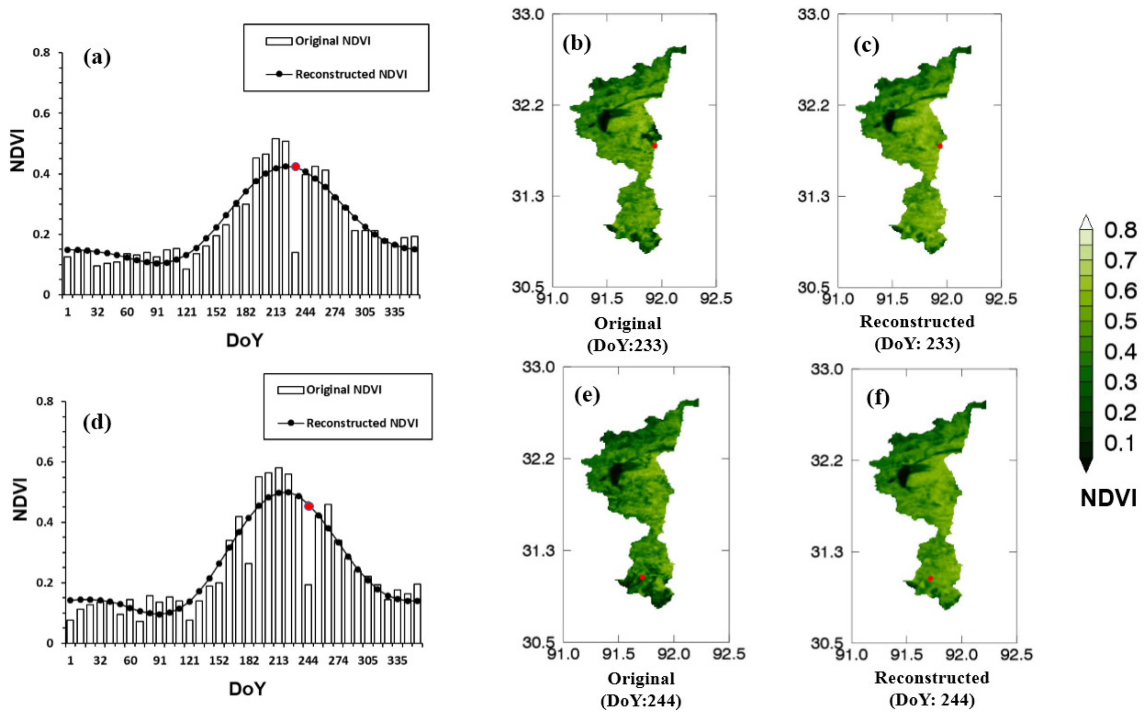
Two different pixels (located at 31.79° N, 91.94° E and 31.09° N, 91.71° E) were chosen randomly for comparison between the original NDVI processed by MVC and reconstructed NDVI by HANTS (
Figure 2). The MVC process was used to recalibrate for the removal of cloud, but some abnormal values caused by residual cloud cover still remain visible in
Figure 2a,d. As can be seen on DOY 233 (
Figure 2a), the NDVI value of the pixel marked by a red point suddenly decreased from 0.45 to 0.1. This signal was recorded as a low NDVI value in blue in
Figure 2b,e. The change took place in a very short time period of 10 days, which was not caused by a vegetation growth process but by clouds. After reconstruction (
Figure 2c,f), some dark green areas diminished and were replaced by normal NDVI values. As shown by
Figure 2a,d, an improved smoothing of time series can be achieved. Negative outliers of NDVI observations that are clearly below the curve due to cloud cover or atmospheric haze, were removed while the characteristics of the original trend was maintained.
4.2. Improvement of Broadband Albedo
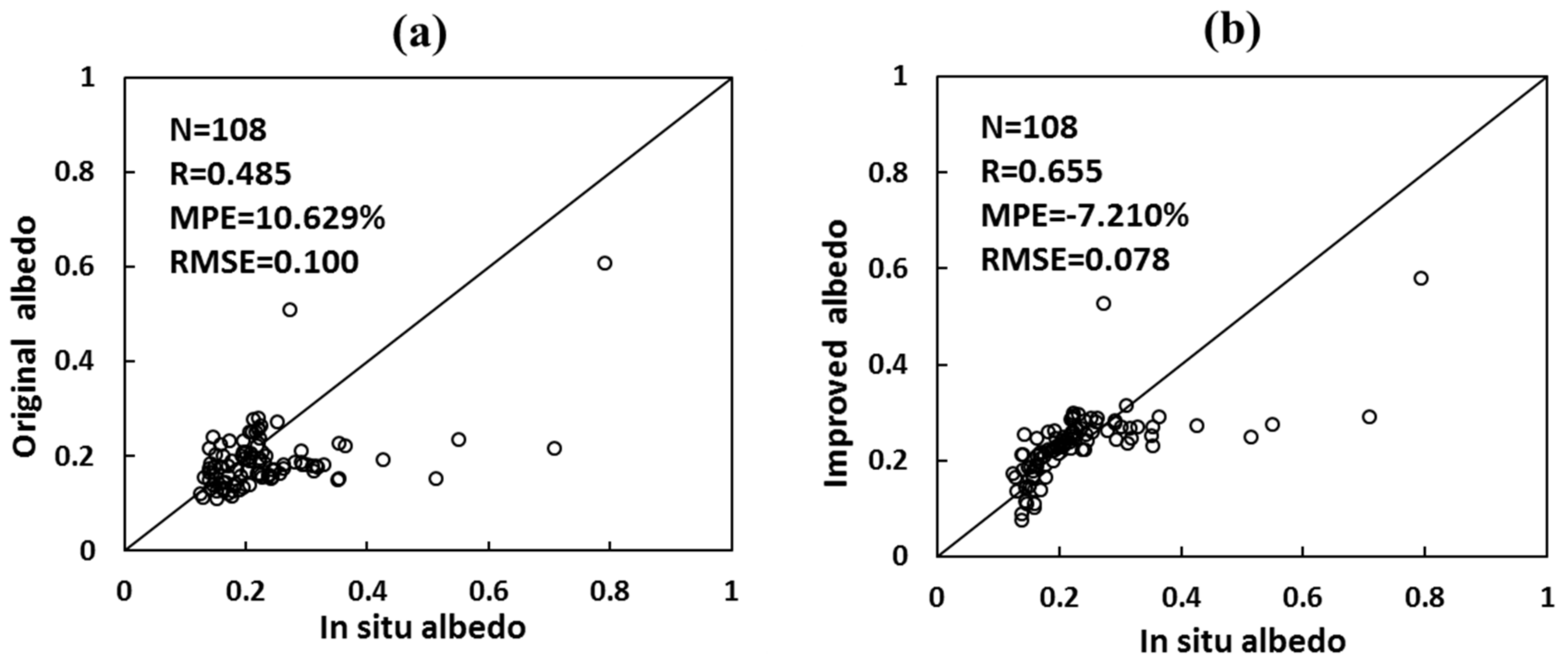
As shown in
Figure 3a,b, the improved method (Equation (2)) has higher R (0.655), lower RMSE (0.078), and MPE (−7.21%) than the original method (Equation (3)) (with R, RMSE, and MPE values of 0.485%, 0.1%, and 10.629%, respectively), which means the new conversion model could provide a better estimation of broadband albedo than the original one. Since snow-covered situations have not been taken into account, some errors might occur when albedo is relatively high. According to global land cover 2000 (GLC2000), the dominant land cover in the study area is alpine and subalpine plain grass. The error of estimated albedo could be large only when snowfall happens, which only takes up a small proportion. This can also be identified from
Figure 3.
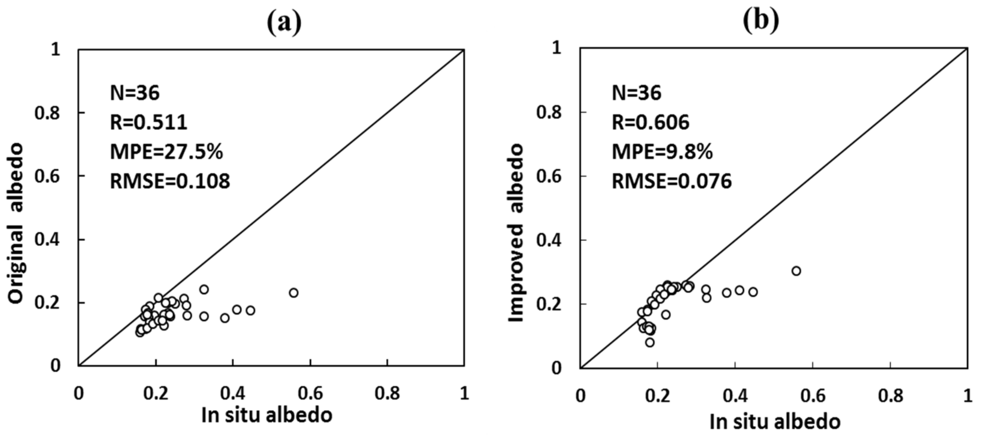
To further validate the improved model, independent observational data from the ANNI station were selected for cross validation (
Figure 4). As shown by
Figure 4a,b, R, MPE, and RMSE of the original method are 0.511, 27.5%, and 0.108 while the statistical indexes from the improved method are 0.606, 9.8%, and 0.076, respectively. Therefore, the improved model could provide a more accurate estimation of broadband albedo in the Nagqu river basin.
4.3. Estimation of Actual Evapotranspiration
Land surface 10-day AET derived from SEBS were validated with the 10-day AET determined using in situ observations taken in the Nagqu river basin (
Figure 5). Since the validation sites are built on relatively flat and homogenous underlying surfaces, the observations are representative of a 1-km pixel. For the time being, how to remove cloud effects on LST and downward radiation flux remains a challenging issue. As shown in
Figure 5, the model-estimated AET values are very close to CM results with R, RMSE, and MPE of 0.972, 0.052 mm/h, and −10.4%, respectively.
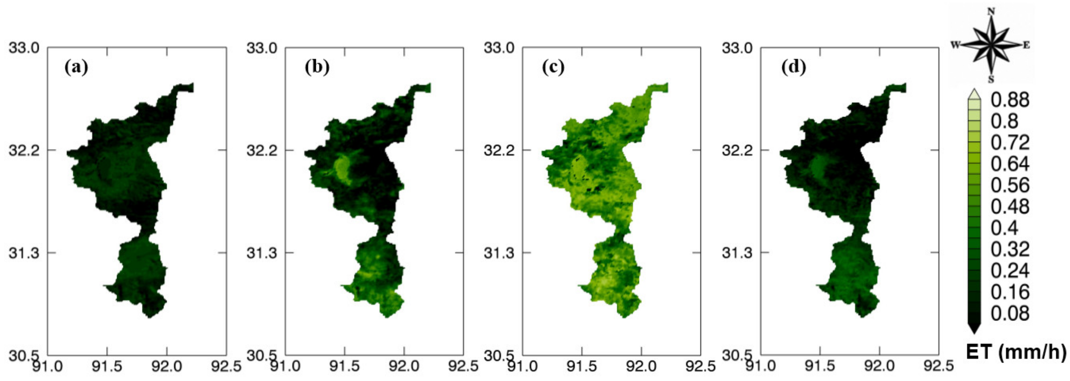
Maps of hourly AET in the Nagqu river basin in January, April, May, and December are shown in
Figure 6. AET in January (0 to 0.29 mm/h,
Figure 6a) and December (0 to 0.43 mm/h,
Figure 6d) were significantly lower than those in May (varies from 0 to 0.77 mm/h,
Figure 6c). Because of the increasing soil moisture during the period of frozen soil melt, AET increases suddenly from April to May, with average AET increasing from 0.184 mm/h to 0.479 mm/h. In the SEBS model, the uncertainty in AET is greatly reduced by taking the energy balance at the limiting cases into account. In comparison with previous studies [
12,
35], which derived the latent heat flux only through LST and surface layer meteorological conditions and are not constrained by limiting cases, the associated uncertainty in the derived ET is small. Moreover, instead of using fixed values as before, the dynamic roughness height for heat transfer was incorporated in SEBS.
5. Discussion
Because of complicated weather conditions over the TP, only several satellite images with total cloud cover less than 40% were used in this study. Although the derived results were generally in agreement with field measurements, some discrepancies still exist. Several reasons may account for this. First, there are errors in the satellite-derived parameters, such as LST, albedo, emissivity, and NDVI. The surface meteorological forcing data of air temperature, humidity, and wind speed also have errors, which has been proved by several studies [
31,
36]. Second, scale issues always exist between satellite-derived results and in-situ measurements [
37]. Since there is no absolute homogenous underlying surface, the error becomes much larger with surface heterogeneity. Third, the SEBS model itself has assumptions and limitations. For example, the model is based on the Monin-Obukhov similarity theory, which produces larger error under stable atmospheric stratification [
17,
18,
30].
The MVC method is widely used to remove cloud cover on satellite images [
38,
39,
40]. It can be used to produce time series of land surface characteristic parameters, such as NDVI, LST, and the leaf area index (LAI) [
21,
25,
41]. However, evidence has shown that artefacts caused by residual cloud cover and atmospheric haze remain visible in MVC-processed time series, which has also been proved in our study. The HANTS algorithm was used to reconstruct one-year cloud-free time series based on the original MVC time series data. The robustness of the HANTS algorithm was confirmed by validating at two different vegetation sites. The HANTS algorithm is superior to other time series processing methods but improvements related to its numerical stability in case of long gaps with no data are still desirable. Taking superiority of the HANTS algorithm into account, we would like to suggest using the above method to further process MVC time series to avoid some uncertainties especially for the estimation of AET and vegetation trend analyses.
The improved land surface characteristic parameter retrieval algorithms, which were incorporated in SEBS in this study, have the potential to be used to derive time series of AET and other land surface heat fluxes (such as sensible heat flux, radiation flux, and soil heat flux) as well. It can also be applied to regions at a larger spatial scale, such as the Tibetan Plateau, China, and even the globe. Additionally, the SEBS model itself can be applied to geostationary satellites to estimate AET with a fine temporal resolution [
18]. The derived AET, together with other components of the water cycle, will help close the water cycle at a basin scale and promote the understanding of energy and the water cycle over the TP. Another good example is that the derived AET and in situ hydrometeorological parameters were used to investigate the inner relationship among AET and energy parameters, hydrological parameters, and dynamical parameters [
5]. The results show that the energy-related factors are most important for the AET in areas with high elevation like the Nagqu river basin. Both the precipitation and wind speed have positive and negative feedback on the AET.
On the application side, SEBS has great potential. It can be suitable for an operational monitoring system if the input forcing data can be provided in a timely manner. SEBS results may be used for initialization or validation of hydrological, meteorological, and ecological models that usually require SEB components at different spatial and temporal scales. The second valuable application is soil water deficit monitoring [
42,
43]. The model can provide actual sensible heat flux as well as sensible heat flux under limiting cases. Although cloud contaminations have been removed successfully in NDVI, albedo, and emissivity data, the application of optical remote sensing data is still limited by cloud contamination because the cloud-contaminated LST and the cloud effects on radiation have not been taken into account yet. In the future, broadband albedo estimation would be improved by taking snow-covered situations into account. Moreover, the estimation of the cloud effects on LST and radiation should be focused on as well. Lastly, more extensive observation networks equipped with eddy covariance instruments need to be constructed over the TP, especially for the vast western region, to provide essential validation information for different satellite estimations and land surface models.
6. Conclusions
In this study, the land surface parameters in the Nagqu river basin, such as NDVI and surface albedo, were retrieved from satellite images. Based on meteorological forcing data and derived land surface parameters, the SEBS model were used to estimate AET with a fine spatial resolution of 1 km. The following conclusions were drawn.
(1) A cloud-free time series of NDVI was successfully reconstructed using the HANTS algorithm.
(2) A land surface broadband albedo parameterization scheme was improved. The albedos derived from the improved method were in good agreement with in situ measurements with a correlation coefficient, a root mean square error, and a mean percentage error of 0.606%, 0.076%, and −9.8%, respectively.
(3) AET with a fine spatial resolution of 1 km was derived in the Nagqu river basin based on the SEBS model with TERRA/MODIS, SPOT/VGT, ASTER/DEM data, and meteorological forcing data as model inputs.
(4) The feasibility and potentiality of using SEBS model to derive mesoscale AET has been tested by comparing it with results from CM in this paper. The validation results indicated that the model-estimated AET agreed well with CM AET with a correlation coefficient, a root mean square error, and a mean percentage error of 0.972, 0.052 mm/h, and −10.4%, respectively.
Author Contributions
L.Z. conceived and designed the study. K.X., X.W., and N.G. performed the experiments and analyzed the satellite data. Y.M. helped in the Evapotranspiration model. K.X., N.G., and Z.H. edited and commented on the manuscript. L.Z. wrote the paper.
Funding
The National Natural Science Foundation of China (41875031), the Strategic Priority Research Program of Chinese Academy of Sciences (Grant No. XDA20060101), the National Natural Science Foundation of China (Grant No. 41522501, 41275028, 91337212, 41661144043, 91837208), the Chinese Academy of Sciences (Grant No. QYZDJ-SSW-DQC019), CLIMATE-TPE (ID 32070) in the framework of the ESA-MOST Dragon 4 Program and Jiangsu Collaborative Innovation Center for Climate Change jointly funded this research.
Conflicts of Interest
The authors declare no conflict of interest.
References
- Mu, Q.; Heinsch, F.A.; Zhao, M.; Running, S.W. Development of a global evapotranspiration algorithm based on MODIS and global meteorology data. Remote Sens. Environ. 2007, 111, 519–536. [Google Scholar] [CrossRef]
- Trenberth, K.E.; Fasullo, J.T.; Kiehl, J. Earth’s global energy budget. B. Am. Meteorol. Soc. 2009, 90, 311. [Google Scholar] [CrossRef]
- Hu, G.; Jia, L.; Menenti, M. Comparison of MOD16 and LSA-SAF MSG evapotranspiration products over Europe for 2011. Remote Sens. Environ. 2015, 156, 510–526. [Google Scholar] [CrossRef]
- Yao, Y.; Liang, S.; Cheng, J.; Liu, S.; Fisher, J.B.; Zhang, X.; Jia, K.; Zhao, X.; Qin, Q.; Zhao, B.; et al. MODIS-driven estimation of terrestrial latent heat flux in China based on a modified Priestley–Taylor algorithm. Agr. Forest Meteorol. 2013, 171, 187–202. [Google Scholar] [CrossRef]
- Zou, M.; Zhong, L.; Ma, Y.; Hu, Y.; Feng, L. Estimation of actual evapotranspiration in the Nagqu river basin of the Tibetan Plateau. Theor. Appl. Climatol. 2017. [Google Scholar] [CrossRef]
- Flohn, H. Large-scale aspects of the ‘summer monsoon’ in South and East Asia. J. Meteorol. Soc. Jpn. 1957, 35A, 180–186. [Google Scholar] [CrossRef]
- Ye, D.; Gao, Y.X. Meteorology of the Qinghai-Xizang Plateau; Chinese Science Press: Beijing, China, 1979. [Google Scholar]
- Wu, G.; Liu, Y.; He, B.; Bao, Q.; Duan, A.; Jin, F. Thermal controls on the Asian Summer Monsoon. Sci. Rep. 2012, 2, 404. [Google Scholar] [CrossRef] [PubMed]
- Immerzeel, W.W.; van Beek, L.P.H.; Bierkens, M.F.P. Climate change will affect the Asian water towers. Science 2010, 328, 1382–1385. [Google Scholar] [CrossRef]
- Ma, Y.; Kang, S.; Zhu, L.; Xu, B.; Tian, L.; Yao, T. Tibetan Observation and Research Platform-Atmosphere-land interaction over a heterogeneous landscape. B. Am. Meteorol. Soc. 2008, 89, 1487–1492. [Google Scholar]
- Mu, Q.; Zhao, M.; Running, S.W. Improvements to a MODIS global terrestrial evapotranspiration algorithm. Remote Sens. Environ. 2011, 115, 1781–1800. [Google Scholar] [CrossRef]
- Jackson, R.D.; Reginato, R.J.; Idso, S.B. Wheat canopy temperature: A practical tool for evaluating water requirements. Water Resour. Res. 1977, 13, 651–656. [Google Scholar] [CrossRef]
- Seguin, B.; Itier, B. Using midday surface temperature to estimate daily evaporation from satellite thermal IR data. Int. J. Remote Sens. 1983, 4, 371–383. [Google Scholar] [CrossRef]
- Bastiaanssen, W.G.M.; Menenti, M.; Feddes, R.A.; Holtslag, A.A.M. A remote sensing surface energy balance algorithm for land (SEBAL): 1. Formulation. J. Hydrol. 1998, 212–213, 198–212. [Google Scholar] [CrossRef]
- Roerink, G.J.; Su, Z.; Menenti, M. S-SEBI: A simple remote sensing algorithm to estimate the surface energy balance. Phys. Chem. Earth. 2000, 25, 147–157. [Google Scholar] [CrossRef]
- Li, Z.L.; Tang, R.; Wan, Z.; Bi, Y.; Zhou, C.; Tang, B.; Yan, G.; Zhang, X. A review of current methodologies for regional evapotranspiration estimation from remotely sensed data. Sensors 2009, 9, 3801–3853. [Google Scholar]
- Han, C.; Ma, Y.; Chen, X.; Su, Z. Estimates of land surface heat fluxes of the Mt. Everest region over the Tibetan Plateau utilizing ASTER data. Atmos. Res. 2016, 168, 180–190. [Google Scholar] [CrossRef]
- Zhong, L.; Ma, Y.; Hu, Z.; Fu, Y.; Hu, Y.; Wang, X.; Cheng, M.; Ge, N. Estimation of hourly land surface heat fluxes over the Tibetan Plateau by the combined use of geostationary and polar orbiting satellites. Atmos. Chem. Phys. 2019, 19, 5529–5541. [Google Scholar] [CrossRef]
- Fisher, J.B.; Tu, K.P.; Baldocchi, D.D. Global estimates of the land-atmosphere water flux based on monthly AVHRR and ISLSCP-II data, validated at 16 FLUXNET sites. Remote Sens. Environ. 2008, 112, 901–919. [Google Scholar] [CrossRef]
- Vinukollu, R.K.; Meynadier, R.; Sheffield, J.; Wood, E.F. Multi-model, multi-sensor estimates of global evapotranspiration: Climatology, uncertainties and trends. Hydrol. Process. 2011, 25, 3993–4010. [Google Scholar] [CrossRef]
- Zhong, L.; Ma, Y.; Salama, M.S.; Su, Z. Assessment of vegetation dynamics and their response to variations in precipitation and temperature in the Tibetan Plateau. Clim. Change 2010, 103, 519–535. [Google Scholar] [CrossRef]
- Yu, W.; Yao, T.; Tian, L.; Wang, Y.; Yin, C. Isotopic composition of atmospheric water vapor before and after the monsoon’s end in the Nagqu River Basin. Sci. Bull. 2005, 50, 2755–2760. [Google Scholar] [CrossRef]
- Yang, K.; He, J.; Tang, W.; Qin, J.; Cheng, C.C.K. On downward shortwave and longwave radiations over high altitude regions: Observation and modeling in the Tibetan Plateau. Agric. Forest. Meteorol. 2010, 150, 38–46. [Google Scholar] [CrossRef]
- Verhoef, W.; Menenti, M.; Azzali, S. Cover. A colour composite of NOAA-AVHRR-NDVI based on time series analysis (1981–1992). Int. J. Remote Sens. 1996, 17, 231–235. [Google Scholar] [CrossRef]
- Julien, Y.; Sobrino, J.A.; Verhoef, W. Changes in land surface temperatures and NDVI values over Europe between 1982 and 1999. Remote Sens. Environ. 2006, 103, 43–55. [Google Scholar] [CrossRef]
- Liang, S. Narrowband to broadband conversions of land surface albedo I: Algorithms. Remote Sens. Environ. 2000, 76, 213–238. [Google Scholar] [CrossRef]
- Becker, F.; Li, Z.L. Towards a local split window method over land surface. Int. J. Remote Sens. 1990, 3, 369–393. [Google Scholar] [CrossRef]
- Zhong, L.; Ma, Y.; Su, Z.; Salama, M.S. Estimation of land surface temperature over the Tibetan Plateau using AVHRR and MODIS data. Adv. Atmos. Sci. 2010, 27, 1110–1118. [Google Scholar] [CrossRef]
- Carlson, T.N.; Ripley, D.A. On the relation between NDVI, fractional vegetation cover, and leaf area index. Remote Sens. Environ. 1997, 62, 241–252. [Google Scholar] [CrossRef]
- Su, Z. The Surface Energy Balance System (SEBS) for estimation of turbulent heat fluxes. Hydrol. Earth Syst. Sc. 2002, 6, 85–99. [Google Scholar] [CrossRef]
- Su, Z.; Schmugge, T.; Kustas, W.P.; Massman, W.J. An evaluation of two models for estimation of the roughness height for heat transfer between the land surface and the atmosphere. J. Appl. Meteorol. 2001, 40, 1933–1951. [Google Scholar] [CrossRef]
- Brutsaert, W. Aspects of bulk atmospheric boundary layer similarity under free-convective conditions. Rev. Geophys. 1999, 37, 439–451. [Google Scholar] [CrossRef]
- Chen, X.; Su, Z.; Ma, Y.; Yang, K.; Wang, B. Estimation of surface energy flues under complex terrain of Mt. Qomolangma over the Tibetan Plateau. Hydrol. Earth Syst. Sc. 2013, 17, 1607–1618. [Google Scholar] [CrossRef]
- Ma, W.; Ma, Y. The annual variations on land surface energy in the northern Tibetan Plateau. Environ. Geol. 2006, 50, 645–650. [Google Scholar]
- Carlson, T.N.; Capehart, W.J.; Gillies, R.R. A new look at the simplified method for remote sensing of daily evapotranspiration. Remote Sens. Environ. 1995, 54, 161–167. [Google Scholar] [CrossRef]
- Han, C.; Ma, Y.; Chen, X.; Su, Z. Trends of land surface heat fluxes on the Tibetan Plateau from 2001 to 2012. Int. J. Climatol. 2017, 37, 4757–4767. [Google Scholar] [CrossRef]
- Ma, Y.; Su, Z.; Koike, T.; Yao, T.; Ishikawa, H.; Ueno, K.; Menenti, M. On measuring and remote sensing surface energy partitioning over the Tibetan Plateau––From GAME/Tibet to CAMP/Tibet. Phys. Chem. Earth 2003, 28, 63–74. [Google Scholar] [CrossRef]
- Holben, B. Characteristic of maximum value composite images for temporal AVHRR data. Int. J. Remote Sens. 1986, 7, 1417–1434. [Google Scholar] [CrossRef]
- Van Leeuwen, W.J.D.; Huete, A.R.; Laing, T.W. MODIS vegetation index compositing approach: A prototype with AVHRR data. Remote Sens. Environ. 1999, 69, 264–280. [Google Scholar] [CrossRef]
- Cuomo, V.; Lanfredi, M.; Lasaponara, R.; Macchiato, M.F.; Simoniello, T. Detection of interannual variation of vegetation in middle and southern Italy during 1985–1999 with 1 km NOAA AVHRR NDVI data. J. Geophys. Res.-Atmos. 2001, 106, 17863–17876. [Google Scholar] [CrossRef]
- Kandasamy, S.; Baret, F.; Verger, A.; Neveux, P.; Weiss, M. A comparison of methods for smoothing and gap filling time series of remote sensing observations-application to MODIS LAI products. Biogeosciences 2013, 10, 4055–4071. [Google Scholar] [CrossRef]
- Su, Z.; Yacob, A.; Wen, J.; Roerink, G.; He, Y.; Gao, B.; Boogaard, H.; van Diepen, C. Assessing relative soil moisture with remote sensing data: theory and experimental validation. Phys. Chem. Earth 2003, 28, 89–101. [Google Scholar] [CrossRef]
- Zhong, L.; Ma, Y.; Fu, Y.; Pan, X.; Hu, W.; Su, Z.; Salama, M.S.; Feng, L. Assessment of soil water deficit for the middle reaches of Yarlung-Zangbo River from optical and passive microwave images. Remote Sens. Environ. 2014, 142. [Google Scholar] [CrossRef]
© 2019 by the authors. Licensee MDPI, Basel, Switzerland. This article is an open access article distributed under the terms and conditions of the Creative Commons Attribution (CC BY) license (http://creativecommons.org/licenses/by/4.0/).


