Abstract
To reveal key parameter-related physical mechanisms in simulating Madden-Julian Oscillation (MJO), seven physical parameters in the convection and cloud parameterization schemes of Beijing Climate Center Climate System Model (BCC_CSM1.2) are perturbed with Latin hypercube sampling method. A new strategy is proposed to select runs with good and poor MJO simulations among 85 generated ones. Outputs and parameter values from good and poor simulations are composited separately for comparison. Among the seven chosen parameters, a decreased value of precipitation efficiency for shallow convection, higher values of relative humidity threshold for low stable clouds and evaporation efficiency for deep convective precipitation are crucial to simulate a better MJO. Changes of the three parameters act together to suppress heavy precipitation and increase the frequency of light rainfall over the Indo-Pacific region, supplying more moisture in low and middle troposphere. As a result of a wetter lower troposphere ahead of the MJO main convection, the low-level moisture preconditioning along with the leading shallow convection tends to be enhanced, favorable for MJO’s further development and eastward propagation. The MJO’s further propagation across the Maritime Continent (MC) in good simulations is accompanied with more land precipitation dominated by shallow convection. Therefore, the above-mentioned three parameters are found to be crucial parameters out of the seven ones for MJO simulation, providing an inspiration for better MJO simulation and prediction with this model. This work is valuable as it highlights the key role of moisture-shallow convection feedback in the MJO dynamics.
1. Introduction
The Madden-Julian Oscillation (MJO), named after its discoverers [1,2], is characterized by a large-scale convection ensemble initiated over India Ocean. Statistically, the MJO propagates eastward slowly (~5 m/s) and dies after crossing the dateline, while the coupled planetary-scale baroclinic circulation still propagates throughout the whole tropical belt at a relatively faster speed [3,4,5]. As the dominant intraseasonal (30–90 days) signal in the tropical atmosphere [6], MJO affects the climate and weather systems over the globe such as the outbreak and withdraw of monsoon systems [3], the initiation of El Niño events [6], the genesis of tropical cyclones [7] and the evolution of extratropical circulation patterns through teleconnection [8,9].
There is a growing body of theoretical work trying to understand the essential physical mechanisms of the MJO [10]. Among the four basic theories, the first one, i.e., the convectively coupled Kelvin-Rossby wave theory was firstly proposed by Wang and Rui [11]. It emphasizes the importance of the interaction between convective heating, the low-frequency equatorial waves, and the boundary layer (BL) frictional moisture convergence. Therefore, only dynamical wave feedback is resolved in this theory [12]. The second basic theory, i.e., the moisture mode theory [13,14,15] regards the atmospheric humidity as the first order important variable under the weak temperature gradient approximation [10]. In this theory, the eastward propagating MJO is simulated by the so-called moisture-convection feedback [16] and moisture transport [17,18,19,20]. The third basic theory, i.e., the frictionally coupled dynamic moisture mode theory combines the above two theories by including a simplified Betts-Miller cumulus parameterization scheme, in which both the moisture-convection [21,22] and wave feedbacks [12] are resolved. The last basic theory, namely, the multiscale interaction theory includes many different schools of thinking about how mesoscale and synoptic-scale disturbances interact and contribute to the MJO dynamics. It includes the MJO skeleton model [23,24,25,26,27,28], the MJO-synoptic wave interaction model; [23,24,26,28], the multi-cloud model [29,30] and the gravity wave interference model [31,32,33]. Besides the aforementioned four groups of basic MJO theories, there are also two specific theories including the boreal summer intraseasonal oscillation (ISO) theory [34] and the atmosphere-ocean interaction theory [35,36,37].
Despite numerously conducted theoretical work trying to understand the MJO dynamics, most of the state-of-the-art climate models still suffer from different hierarchies of deficiencies of simulating realistic MJO structure and its eastward propagation [38,39,40,41,42,43]. Hung et al. [44], for example, demonstrated that only about one-third of the General Circulation Models (GCMs) from the Coupled Model Intercomparison Project phase 5 (CMIP 5) generate the spectrum peak of MJO precipitation between 30 and 70 days. Among them only one model produces the realistic eastward propagation. Jiang et al. [41] found that only one-fourth of the latest-generation GCMs could accurately simulate the systematic eastward propagation of MJO. These highlight the necessity to advance our understanding of the potential mechanisms in shaping the fundamental behaviors of the MJO, especially its smooth propagation from the Indian Ocean to the western Pacific seen in the observation statistics [2,45,46].
An important factor leading to the unrealistic MJO simulations in GCMs has been widely recognized as the uncertainty in cloud and convection parameterization schemes, which largely resolve atmospheric subgrid-scale moist and convective processes [43,47,48,49]. For example, by increasing the minimum value of cumulus entrainment rate of the environmental air in the Arakawa-Schubert (AS) cumulus convection parameterization scheme, the equatorial intraseasonal signals are better simulated by GCMs [50]. Wang and Schlesinger [51] demonstrated that the simulated Intraseasonal Tropical Oscillation (ITO) becomes stronger by increasing relative humidity criterion for convective heating () in three different parameterization schemes using one GCM model. The effects of convective precipitation evaporation in unsaturated environmental air and unsaturated downdrafts are found to be essential for the amplitude of simulated MJO in GCM [52]. The role of stratiform precipitation portion in MJO simulation is investigated in Fu and Wang [53] and results show that increasing the portion of stratiform precipitation by changing the value of deep or shallow convection detrainment rate leads to a robust MJO in GCM. A robust relationship between environmental moisture and convection was also confirmed in observation [54] and models [55,56].
In this study, we seek to find out certain cloud and convection parameter perturbations leading to models’ best and worst ability of simulating MJO so that the parameter-related physical processes crucial for MJO simulation could be found. Therefore, we perturb seven control parameters (such as the moisture thresholds related to convection trigger, the low and high stable clouds, the efficiencies related to precipitation and evaporation in deep and shallow convections, and the adjustment timescale for shallow convections) in the cloud and convection parameterization schemes, using Beijing Climate Center Climate System Model (BCC_CSM1.2) with a revised Zhang and McFarlane’s convection scheme (hereafter RZM) [49,57]. Therefore, a variety of model runs are generated after perturbing these parameters in order to identify parameter perturbations leading to runs with a high-skill MJO simulation (hereafter good simulations) and runs with a low-skill MJO simulation skill runs (hereafter poor simulations).
The parameter perturbation strategy and model used in this study is the same as that in Liu et al. [57], but for different purposes. Liu et al. [57] focused on the optimization of MJO simulation and prediction skills, while this study emphasizes the crucial physical mechanisms for better MJO simulation, which are modulated by values of cloud and convection parameters in this model. Besides, to objectively select the good and poor integrations, a new evaluation strategy for the MJO simulation skill is proposed in this study. Unlike Liu et al. (2018) who only select one high-skill run and one low-skill run, this study would objectively identify those good and poor simulations with the new evaluation strategy, and a composite analysis is then performed for the two groups of simulations. In this way, a robust result may be shed light on, and more importantly, the parameter-related mechanisms that are vital important to the better MJO simulations will be revealed in a robust way.
This paper is arranged as follows. Section 2 describes the data and methodology. The composite good and poor simulations of the MJO are presented in Section 3. The diagnostics of mean states are given in Section 4. Section 5 analyzes the MJO-scale cloud and moist processes, in which the key role of moisture and shallow convection feedbacks are identified and studied. Finally, the summary and discussion are given in Section 6.
2. Data and Methodology
2.1. Data
BCC_CSM1.2 model [58] is used in this study. BCC_CSM1.2 model is a climate system model including 4 components. The atmospheric component of BCC_CSM1.2 is Beijing Climate Center Atmospheric General Circulation Model (BCC_AGCM3.0), which adopts a spectral truncation of 106 waves (T106) in the horizontal and 40 layers (L40) in the vertical from surface to 0.31 hPa. Beijing Climate Center Atmosphere-Vegetation Interaction Model (BCC_AVIM2.0) [59] is used as BCC_CSM1.2’s land surface component with the same horizontal resolution as BCC_AGCM3.0. The global ocean general circulation model in BCC_CSM1.2 called MOM4_L40v2 is modified from the Modular Ocean Model (MOM4) to include the ocean carbon cycle [59] with a horizontal resolution of 1/3 degrees (~30 km) and 40 vertical layers. BCC_CSM1.2 also includes the Sea Ice Simulator (SIS) [60] as its sea ice model.
The RZM scheme invoked in our work is a revised version of the original scheme of Zhang and McFarlane [48]. It is different from the original scheme in (a) the closure condition, where the original scheme only assumes that convection acts to remove the atmospheric convective available potential energy with a relaxation of 2 h while the RZM assumes that a quasi-equilibrium exists between convection and the large-scale environment in the free troposphere above the boundary layer, (b) the inclusion of a relative humidity threshold for convection triggering, which acts to suppress spurious convection when the boundary layer is dry, and (c) the allowance for the bottom of the unstable lifted layer’s occurrence above the boundary layer. Details about the revision could be found in Zhang and Mu [49] and Wu et al. [61].
A series of experiments were run by perturbing the values of (1) adjustment time scale for shallow convection (), (2) precipitation efficiency for shallow convection (), (3) relative humidity threshold for low stable clouds (), (4) relative humidity threshold for high stable clouds (), (5) relative humidity threshold for convection trigger (), (6) precipitation efficiency for deep convection () and (7) evaporation efficiency for deep convective precipitation () [57]. These parameters are perturbed with Latin Hypercube sampling (LHS) method [62] to sample points within the seven-dimensional parameter space. The Latin hypercube procedure selects pseudo-random points from the full seven-dimensional parameter space, ensuring uniform coverage across the space. Details of the experimental design could be found in Section 2.2.1 of Liu et al. [57].
Adopted from Liu et al. [57], Table 1 shows the default, maximum and minimum values of seven chosen parameters. In total, 85 perturbed points or 85 sets of different parameter values are sampled for seven parameters. The model is integrated with each set of parameters for seven years, generating 85 sets of daily outputs on grids with a horizontal resolution of 1.125° × 1.125° at 40 vertical layers. Considering that these integrations may take a few years to reach an equilibrated state after changing values of these seven parameters, we examined the time series of tropical (30° S–30° N) Surface Temperature and column-integrated (850–500 hPa) specific humidity in the 85 integrations (not shown here). Results show that most of the integrations reach an equilibrated state after 1.5–2 years of adjustment. Therefore, the last five years of each set of outputs are used for analysis.

Table 1.
Description, default values and perturbed ranges of seven parameters in the model, adopted from Liu et al. [57].
The observational data used in this study consists of the daily outgoing longwave radiation (OLR) data from the National Oceanic and Atmospheric Administration (NOAA) polar-orbiting series of satellites [63], TRMM based precipitation observations (version 3B42 v7) [64] and the European Center for Medium-Range Weather Forecasting (ECMWF) ERA-Interim reanalysis [65] for the period of 2000–2009. All datasets and model outputs are interpolated into a 2.5° × 2.5° longitude-latitude grid and 19 vertical layers as ERA-Interim reanalysis data.
2.2. Methodology
2.2.1. Evaluation of MJO Simulation with Three Canonical Methods
Many metrics regarding MJO variability and its internal physics have been given in previous studies [41,42,44,45,55,66,67,68,69]. Jiang et al. [41] proposed two metrics to evaluate the models’ ability of simulating realistic MJO. The first approach (Lag-correlation hereafter) is defined as the average value of two pattern correlation coefficients (PCCs) in each model. The equatorial (10° S–10° N) 20–100–day filtered precipitation in GCM outputs and observation are lag regressed from day -20 to 20, against the area-averaged time series of itself over India Ocean (75–85° E; 5° S–5° N) and Pacific Ocean (130–150° E; 5° S–5° N), respectively. Two regional Hovmöller plots (day −20 to 20, (60° E–180°)) are given in each GCM and observation by averaging the regressed precipitation in meridional direction. Two PCCs are computed by regional Hovmöller plots in GCM and observation. The averaged value of these two PCCs is thus defined as the MJO simulation skill score by Lag-correlation. The other approach is based on the regional (60° E–180°) space-time power spectral analysis of precipitation or other convection related variables over an equatorial belt [70], and it is defined as the ratio of the spectral power for the eastward to westward propagation component (E/W ratio hereafter) on MJO time and space scales (period of 30–90 days, zonal wavenumber of 1–3). Another approach called “MJO tracking method” is also used to examine the MJO simulation qualities in different models in previous study [42]. It is based on the Hovmöller diagrams of filtered equatorial precipitation. A set of criteria is used to track the MJO events in model outputs. Each event’s amplitude, propagation range and life span are also given by this method. Details about the MJO tracking method could be found in Zhang and Ling [71].
Three aforementioned approaches (Lag-correlation, E/W ratio and MJO tracking method) are used to examine the MJO simulation skills in 85 integrations. It is worth noting that the Lag-correlation and E/W ratio scores are computed based on the OLR data, considering that OLR is a good representation of organized convection systems and has a normal distribution. However, the MJO tracking method is still based on equatorial precipitation data because this method includes some criteria especially designed by using precipitation data like the reference longitude and the criteria used to determine the initiating and ending date of each MJO event [71]. Using OLR in MJO tracking method without changing these criteria leads to its failure to track MJO events. Therefore, we still use precipitation data in the MJO tracking method for convenience. Figure 1 shows the scores of 85 integrations given by Lag-correlation. Runs of the top 10 and bottom 10 scores are labeled in red and blue, respectively. The top (bottom) 10 is then identified as stronger (weaker) MJO runs. Compared with the result in Jiang et al. [41], the diversity of scores in our study is clearly smaller with most of them lying between 0.7 and 0.85. The E/W ratio scores computed with OLR are given along with the Lag-correlation scores in Figure 2a. Integrations identified as strong (weak) MJO simulations are scattered in red (blue). The E/W ratio scores in all 85 runs are above 1.0, indicating that the eastward propagating components of large-scale intraseasonal signals in 85 integrations are stronger than that of the westward propagation component. However, the correlation coefficient between Lag-correlation scores and E/W ratio scores is only 0.23, and the stronger MJO integrations identified by Lag-correlation scores lie in almost the same zone in E/W ratio as weaker MJO integrations. The linear fit between two scores also shows that two scores no longer corroborate each other in MJO simulation skill measurement. Considering that the Lag-correlation scores are computed with OLR data filtered only in time dimension while OLR data is filtered both in time and zonal dimension before computing E/W ratio scores, the E/W ratio in the same times scale of 30–90 days but at different wavenumbers of 1–15, and 4–15 are computed, as shown in Figure 2b,c, along with Lag-correlation scores. The regression lines in Figure 2b,c are much steeper compared with that in Figure 2a, but it is probably due to the narrower spread of E/W ratio values in the x axis. The correlation coefficient between these two scores slightly increases when including intraseasonal signals of all zonal wavenumbers. The correlation coefficient decreases to 0.13 if only a wavenumber of 4–15 spectral power is included to compute the E/W ratio.
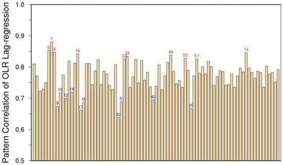
Figure 1.
Scores of 85 integrations by Lag-correlation defined as the average values of two pattern correlation correlations (PCCs) in each run. The PCCs of each run are computed between the Hovmöller diagrams in it and observation, which are given by averaging equatorial (10° S–10° N; 60° E–180°) lag regressed 20-100 day filtered outgoing longwave radiation (OLR) from day −20 to 20 against the area-averaged time series of itself over India (5° S–5° N; 75° E–85° E) and Pacific (5° S–5° N; 130° E–150° E). The highest (lowest) 10 runs are labeled with their experiment identification number in red (blue).
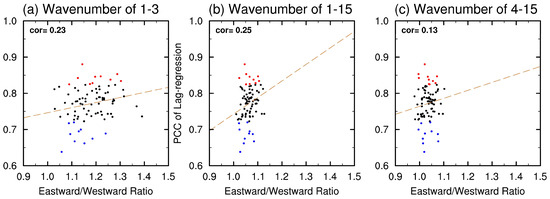
Figure 2.
Scatter plot of scores by Lag-correlation (y axis) against scores by E/W ratio (x axis) of zonal wavenumber (a) 1–3, (b) 1–15, and (c) 4–15. The scores by Lag-correlation are the same as those in Figure 1. Scores by E/W ratio are defined as the values of dividing the spectra power in the eastward-propagating component by that in the westward-propagating component on MJO time and space scales (period of 30–90 days, zonal wavenumber of 1–3) in each run. The power spectral analysis is conducted with regional OLR (5° S–5° N; 60° E–180°) and then averaged meridionally. The 10 integrations identified by Lag-correlation as with stronger (weaker) MJO are scattered in red (blue) while the others in black. The dot line donates the linear fit by least squares means. The correlation coefficients are also displayed.
The same diagrams are done to investigate the correlation between scores given by quantities of MJO events, Lag-correlation and E/W ratio. Ling et al. [42] proposed a hypothesis after evaluating 27 GCMs that the model’s ability of simulating MJO is highly related to the quantity of MJO events in model integration. The more frequent model produces MJO events, the higher MJO simulation skill the model has. Therefore, MJO tracking method is applied to get the quantity of MJO events in 85 integrations. Figure 3 presents the same scatter plots as Figure 2 but with X axis referring to the quantity of tracked MJO events in 85 integrations and Y axis referring to E/W ratio scores in Figure 3a–c, and Lag-correlation scores in Figure 3d. Among 4 correlation coefficients in scatter plots of Figure 3, the correlation coefficient between quantities of MJO events and E/W ratio is the highest, but only reaching 0.26. The low correlation coefficients in Figure 3 indicate that scores given by quantity of MJO events do not corroborate with those given by Lag-correlation, nor E/W ratio.
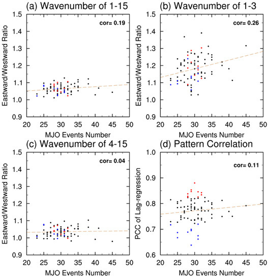
Figure 3.
Same as in Figure 2 but with x axis denotes the quantity of MJO events in model integration given by MJO tracking method. y axis donates to scores by E/W ratio of wave number (a) 1–15, (b) 1–3, (c) 4–15 and scores by Lag-correlation in (d).
2.2.2. A New Strategy to Evaluate the MJO Simulation Skill
A new evaluation strategy is therefore proposed to identify integrations with good and poor MJO simulations. The contradiction in scores using the above three different canonical approaches individually makes it difficult to find out one certain integration with the highest MJO modulation skills in all respects. However, the two approaches (Lag-regression and E/W ratio) in Jiang et al. [41] are still widely used to evaluate model’s MJO simulation skills. The Lag-correlation examines the propagation quality of intraseasonal signals while E/W ratio investigates whether the eastward propagation is dominant in MJO time and space scales. Therefore, a combination of Lag-regression and E/W ratio scores is used to identify good simulations and poor simulations. The new evaluation strategy consists of three steps: (i) rank 85 integrations twice, in order of Lag-correlation and E/W ratio scores respectively from high to low, (ii) divide two ranks respectively into three tiers (the top, middle and bottom tiers). Two rank’s top and bottom tier sizes (hereafter tier-size) are same. (iii) identify good and poor simulations. If one integration lies in top (bottom) tier of both two ranks, this integration is thought to be good (poor) simulation.
Attempts are made to choose the appropriate tier-size during dividing two ranks into three tiers in step ii. Three rules need to be considered while choosing: (i) the quantities of selected good and poor simulations should be sufficient to do the composite analysis, (ii) the difference between the case numbers of selected good and poor simulations is small enough to fairly compare the composite results, and (iii) the mean scores in good and poor simulations show distinct differences. Figure 4 shows the quantities of selected good and poor simulations and the difference between mean scores of these two groups according to different tier-sizes. Based on the second rule, tier-size of 10, 20 and 33 are worth considering. However, the quantities of selected good and poor simulations are too small to do the composite analysis when tier-size is under 16 and the difference between mean scores decreases rapidly when tier-size is greater than 20. Therefore, we choose 20 as the appropriate tier-size by which six good simulations (integration 1, 6, 23, 33, 38 and 48) and eight poor simulations (integration 10, 14, 18, 30, 43, 45, 55 and 70) are identified for the following analysis. Distributions of MJO scores are analyzed to investigate the validity of this new strategy. Figure 5 presents the distribution of good and poor simulations selected by this new strategy in scores of Lag-correlation and E/W ratio among 85 integrations. Uniform higher scores could be seen in good simulations compared with poor ones, especially of E/W ratio scores, indicating that such new evaluation strategy is effective in selecting high-skill and low-skill MJO simulations.
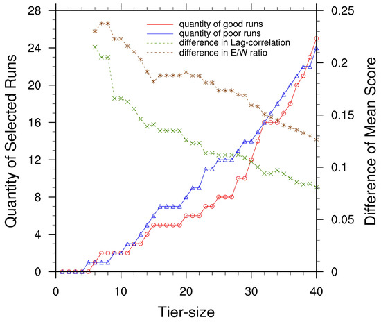
Figure 4.
Quantities of selected good and poor simulations (left y-axis) and differences between mean scores of selected good and poor simulations (right y-axis) according to different values of tier-size.

Figure 5.
Scatter plots of scores by Lag-correlation (y axis) against scores by E/W ratio (x axis) with good (poor) simulations selected by the new evaluation strategy scattered in red stars (blue triangles) while the rest of 85 runs scattered in black dots.
2.2.3. Compositing Technique and Significance Test
Before the composite analysis, a linear regression technique was conducted for each group of simulation. The referenced time series is calculated as the 20–100-day, bandpass-filtered OLR anomaly averaged over the Indian Ocean (5° S–5° N; 75°–85° E) and Pacific Ocean (5° S–5° N; 130°–150° E). Then, the MJO-scale perturbations are obtained by regressing any atmospheric or oceanic parameters against this referenced time series. The composite results of the six good simulations and eight poor simulations are calculated using their associated regression patterns, respectively, in which the lags from −20 to 20 days is used to thoroughly observe the entire life cycle of the MJO. The significance test of the composite results at the 90% confidence level is based on the Student’s t statistic that obeys a distribution with a degree of freedom (DOF) of N. The DOF N is 6(8) for the good (poor) simulations.
3. Composites of Good and Poor Simulations
3.1. Parameter Values
Average values of seven chosen parameters in good and poor simulations are given in Figure 6. Seven chosen parameters differ largely in their magnitudes as Table 1 shows. In order to visualize each parameter’s perturbation in good and poor simulations and to compare their differences, the values of these parameters are converted to their percentiles in each parameter’s changing range (maximum-minimum as in Table 1). Three parameters such as precipitation efficiency for shallow convection (), relative humidity threshold for low stable clouds () and evaporation efficiency for deep convective precipitation () exhibit significant differences between good and poor simulations. In good simulations, values of and are about twice of those in poor simulations while the value of is only about the one third of it in poor simulations.
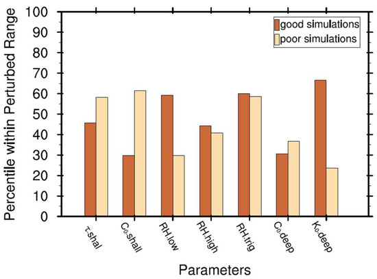
Figure 6.
Average values of 7 chosen parameters in good and poor simulations in form of each parameter value’s percentile within its perturbing range (maximum-minimum) as in Table 1.
Individual changes in values of the above three parameters lead to changes in cloud and convection. Increasing RH threshold for low stable clouds value leads to a reduction of low-level clouds, and this reduction results in an additional moisture accumulation beneath low stable clouds. The decrease in value of precipitation efficiency for shallow convection makes it harder for water in shallow convective clouds to convert to rain droplets. Therefore, this would decrease the shallow convective precipitation and thus humidifying the low troposphere. The sharp increase in the value of evaporation efficiency for deep convective precipitation causes a higher ratio of deep convective rain droplets evaporating while falling down. So, the deep convective precipitation declines largely due to this change. Interestingly, research shows that this change not only influences the deep convection, but also is favorable for low cloud formulation and development of shallow convection [72]. In general, the sharp contrasts between good and poor simulations in terms of these three parameter values have implied the crucial role of the lower-tropospheric moistening in supporting the better MJO simulation (e.g., Yoneyama et al. [73]; Wei et al. [74]).
3.2. Zonal Wavenumber-Frequency Spectrum
To check the characteristics of MJO along with other Convection Coupled Equatorial Waves (CCEWs), Figure 7 shows the signal-to-noise ratio of OLR anomalies computed using the space-time spectral analysis method [70]. In observation, three main CCEWs are clearly shown in Figure 7a. Westward-propagating Equatorial Rossby (ER) waves are dominant in low-frequency period of wavenumbers 3–5 while eastward-propagating Kelvin waves and MJO are also identified. The spectral band of MJO signals lies within zonal wavenumbers of 1–3 and timescales of 30–90 days, with a single peak at wavenumber of 1 and frequency of 0.15 cycles per day (period of 40 days). The timescales of Kelvin waves in observation vary between three days and 15 days with greater zonal wavenumbers of 2–8. The gap between Kelvin waves and MJO in the power spectral is distinct in observation. Figure 7b presents the composite result of spectral analysis in poor simulations. Compared with observation, the ER waves in poor simulations exhibit a new independent power center at wavenumber 6. MJO-related signals greatly shrink and are divided into two individual peaks (at wavenumber 1 and 4) with a much weaker amplitude. Kelvin waves are not well simulated in poor simulations. Kelvin waves vanish in shorter timescales and larger zonal wavenumbers. The residual part of Kelvin wave is connected with weak MJO, filling the gap between them in observation. Composite result of good simulations shows improvement in simulation of CCEWs. MJO-related signals are amplified with a center at zonal wavenumber 1 compared with poor simulations. Kelvin waves are also improved by enhancing the spectral power of its fast components with larger zonal wavenumbers. The improvement of Kelvin waves accompanied with better MJO in models is also proposed in the previous study [75,76]. ER waves are also improved by eliminating the positive bias in zonal wavenumber 6 of westward-propagating component.
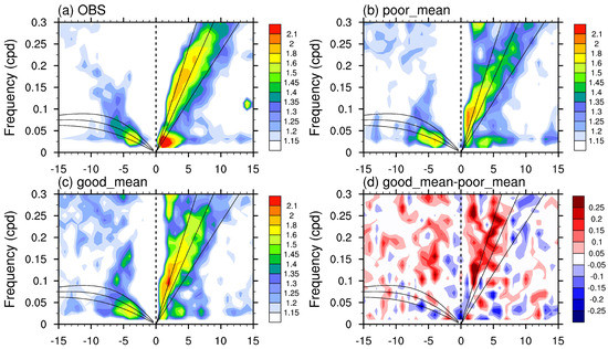
Figure 7.
Boreal-winter (November–April) Signal-to-noise ratio in the wavenumber–frequency spectral domain of the 15° S–15° N symmetric components of OLR anomalies in (a) observation, (b) composite of poor simulations, (c) composite of good simulations and (d) difference between composited results of good and poor simulations.
3.3. Hovmöller diagrams
In order to investigate the propagation of intraseasonal convection systems, the boreal winter Hovmöller diagrams in observation, good and poor simulations are given in Figure 8. The equatorial (10° S–10° N), 20–100-day band-pass-filtered OLR in boreal winter is lag-regressed form day −20 to 20, against the time series of itself averaged over equatorial India Ocean (75°–85° E; 5° S–5° N) and west Pacific (130°–150° E; 5° S–5° N), respectively. The three-dimensional coefficient is then averaged in meridional direction to obtain the Hovmöller plots. In observation as Figure 8a,b show, the convection systems are initiated over Indian Ocean. Well-organized eastward propagation is produced over both India and Pacific Ocean at a speed of about 5 m/s. The barrier effect of Maritime Continent on MJO’s propagation is also indicated in Figure 8b with the propagation slowed down while crossing. In poor simulations given by Figure 8c,d, the regressed coefficient exhibits a strong westward-propagating feature over India Ocean. The propagation over Pacific is relatively better with a weaker westward-propagating component, but the MJO convection dies quickly before reaching the dateline. Also, discontinuous signals are generated after day 0 over west Pacific to motivate the eastward propagation faster than observation. While in good simulations as Figure 8e,f show, the propagation of intraseasonal convection systems is improved both over India and Pacific Ocean. The westward propagations over India Ocean in poor simulations are eliminated. A new eastward-propagating convection signal occurs over Maritime Continent a few days after day 0, indicating that the intraseasonal convection initiated over India Ocean propagates further across MC in good simulations. These improvements have reached 90% confidence level. The improvement of MJO convections over Pacific Ocean is relatively weaker with a continuous signal developed at lag day −10 propagating eastward at almost the same speed in observation. The propagation range over Pacific Ocean in good simulations also gets improved with convections triggered at or even east of dateline, similar with the observational situation.
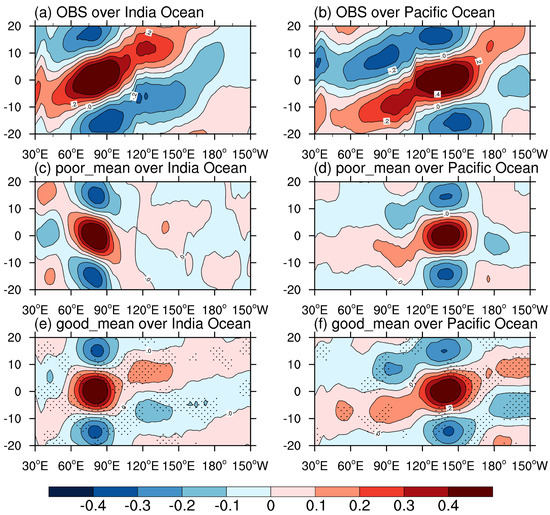
Figure 8.
Boreal winter (November–April) Lag-longitude cross section of the correlation coefficient of 20–100 day filtered OLR anomalies against the area-averaged time series of itself in observation (a and b), poor simulations (c and d) and good simulations (e and f) at the reference area of equatorial India Ocean (5° S–5° N; 75°–85° E) (left column) and Pacific Ocean (5° S–5° N; 130°–150° E) right column). The regressed coefficient is averaged over 10° S–10° N. (d) and (e) are dotted where the difference between composite of good and poor simulations reach 90% confidence level.
4. Diagnostics of Climatology
4.1. Mean State
Previous studies of the MJO concluded that a reasonable mean state is necessary to simulate realistic MJOs [41,77]. Figure 9a–d show the winter-mean precipitation in the composite of poor simulations, the composite of good simulations, observation and the difference between good and poor composites, respectively. As shown in Figure 9a, poor simulations suffer from the problem of double inter-tropical convergence zone (ITCZ). Insufficient precipitation occurs over the Maritime Continent and the east boundary of the Bay of Bengal. Excessive precipitation is dominant in the South Pacific Convergence Zone (SPCZ) and southwest India Ocean. After changing the values of seven parameters, the composite pattern of climatological-mean precipitation in good simulations does not change much in the overall distribution. However, the composite of good simulations is improved by amplifying rainfall in Maritime Continent, mainly over land. The positive biases over SPCZ and south India Ocean are also amplified. In order to better examine the boreal winter mean state, the winter-mean Sea Surface Temperature (SST), u850 and integrated low-level (850–500 hPa) specific humidity in poor simulations, good simulations, observation and the differences between good and poor simulations are given in Figure 10. Both the tropical SST and integrated specific humidity experience an overall increase in good simulations compared with poor simulations, which is consistent with the finding in previous researches that there will be more MJO events with a greater amplitude and farther propagation in a warmer and wetter world [78,79]. It is worth noting that the rise of low-level integrated specific humidity increases the meridional gradient of mean humidity. It has been proposed in Gonzalez and Jiang [80] that a steeper meridional mean humidity gradient is favorable for MJO propagation. The difference of u850 between good and poor simulations shows that the equatorial westerly over India and west Pacific gets amplified. However, the easterly south of MC is also strengthened.
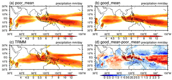
Figure 9.
Winter-mean precipitation in (a) composite of poor simulations, (b) composite of good simulations, (c) observation and (d) the difference between composites of good and poor simulations with that reaching 90% confidence level dotted.
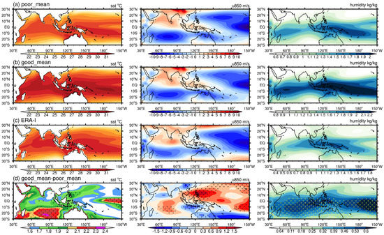
Figure 10.
Boreal winter (November–April) mean state of Sea Surface Temperature (SST, left column), 850 hPa zonal wind (u850, middle column) and integrated low-level (850–500 hPa) specific humidity in (a) composite of poor simulations, (b) composite of good simulations, (c) observations and (d) the differences between composites of good and poor composites. The differences reaching 90% confidence level are dotted in (d).
The occurrence frequency of background precipitation is also examined because researches find out that contemporary climate models used in Phase 3 and Phase 5 of the Coupled Intercomparison Project have biases in the frequency distribution of tropical rainfall inhibiting complete formation of the tropical convective cloudiness [55,81]. The distribution of rainfall over the equatorial Indo-Pacific region (10° S–10° N; 50° E–180°) as a function of accumulated percentiles (divided by the lower 80th and upper 20th percentiles) is given in Figure 11. Light rainfall is defined with amplitude of 0.1–10 . With no precipitation accounts for almost 0% in composite results of both good and poor simulations, the percentile of light rainfall accounts for 80% in poor simulations, the same as observation although the frequency distribution varies. Composite result of the poor simulations shows large bias in the accumulated percentile distribution of rainfall less than and more than , which indicates an insufficient generation of extremely light precipitation (less than ) and excessive generation of intense precipitation in poor simulations. This bias is largely corrected in good simulations with both ends of the distribution curve closer to observation, especially for intense precipitation. Therefore, the frequency distribution of precipitation over the equatorial Indo-Pacific region is much improved by changing the values of seven parameters.
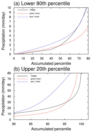
Figure 11.
Histogram of precipitation () in equatorial Indo-Pacific region (10° S–10° N; 50° E–180°) as a function of accumulated percentiles. (a) Lower 80th percentile and (b) upper 20th percentile are plotted.
4.2. Environmental Moisture Sensitivity of Convection
To examine the relationship between moisture and convection closely, composite vertical profiles of the Relative Humidity (RH) as a function of daily averaged precipitation over the Indo-Pacific region are given in Figure 12. In the observation (Figure 12a), the lower troposphere becomes more humid as the precipitation rate increases. The entire column is almost saturated when the precipitation rate is greater than 10 , which means that the heavier precipitation is suppressed until the atmosphere is almost saturated with relative humidity higher than 70%. It is similar to previous findings that more convection occurs in a more humid atmosphere [54,55]. Composite result of poor simulations in Figure 12b shows a dryer environmental atmosphere for light rainfall. Precipitation greater than 30 in poor simulations occurs with a more humid environment at levels around 350 hPa while the lower and upper troposphere are still dryer than observation. The dry bias indicates that the excessive intense precipitation as in Figure 11b consumes too much moisture in the environmental atmosphere. Therefore, most convections in poor simulations develop in a dryer atmosphere. The difference between composite results of good and poor simulations are presented in Figure 12d. The entire lower atmosphere (840–500 hPa) witnesses a moistening with a center at 600 hPa of all precipitation intensities while the humidifying center lies within light precipitation rates (0.1–10 ). This is consistent with changes in rain rate frequency over the same region in Figure 10, where more frequent extremely light rainfall and less heavy precipitation could be seen in good simulations.
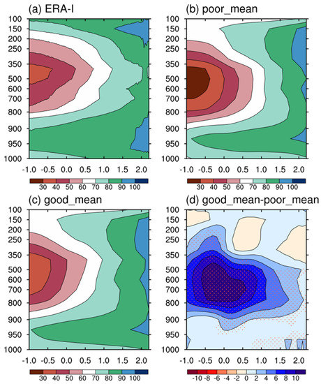
Figure 12.
Composite vertical profiles of relative humidity as a function of precipitation rate over equatorial Indo-Pacific region (10° S–10° N; 50°–180° E) in (a) observation, (b) composite of poor simulations, (c) composite of good simulations and (d) the difference between composites of good and poor simulations. The differences reaching 90% confidence level are dotted. Noted that the precipitation rate on x axis is plotted on a scale.
Difference in the moisture-convection relationship between good and poor simulations is probably due to large changes in values of three important parameters. Increasing the evaporation of deep convective precipitation is favorable for the development of shallow convection [72]. While increasing the value of RH threshold for low level stable cloud and decreasing the value of shallow convective precipitation efficiency both tend to reduce shallow convection, this reduction is compensated with the effect of humidifying low troposphere by intensifying deep convective rainfall evaporation. More shallow convection in good simulations in Figure 11 transports moisture in the low troposphere to middle level, humidifying middle troposphere and drying low troposphere. However, rigorous conversion from cloud water to shallow convective precipitation and less low cloud both lower the efficiency of low-level moisture consumption due to shallow convective precipitation, thus accumulating more moisture in low troposphere. Superimposition of all above influences results in an overall humidifying centering at middle troposphere of light precipitation.
5. Role of Moisture-Shallow Convection Feedback
5.1. Pre-Moistening Effect over the Lower-Layer Atmosphere
Profile of boreal winter regressed specific humidity at lag day 0 is diagnosed to investigate the changes in the MJO-related moisture structure. Figure 13 shows profiles of equatorial (10° S–10° N) specific humidity anomalies regressed against the 20–100 day filtered OLR time series in the reference area (5° S–5° N; 75°–85° E) in observation, good simulations, poor simulations and the difference between good and poor simulations. Result in observation given in Figure 13a shows a west-tilted structure of MJO convection system. The leading preconditioning moisture in lower troposphere and boundary layer ahead of the main convection plays an essential role in the eastward propagation of MJO (e.g., Kim et al. [77]; Hsu and Li [82]; Zhao et al. [83]; Hsu et al. [84]; Wang et al. [85]; Wei et al. [74]). Such preconditioning moisture destabilizes lower troposphere, favorable for the development of leading shallow convection. The shallow convection develops into the following deep convection of the MJO main convection system, resulting the systematic eastward propagation. Figure 13b presents the profile of regressed moisture in poor simulations. The west-titled structure in observation turns into a straight one in poor simulation centering at middle troposphere with broken weak signals ahead, which accounts for the non-propagating or even westward propagating intraseasonal convection systems as Figure 8c,d indicate. As Figure 13d presents, the difference between profiles of regressed equatorial moisture in good and poor simulations tends to compensate for the large bias in poor simulations mainly by moistening the lower troposphere and boundary layer ahead of the main convection of MJO. Therefore, the pre-moistening at low-layer troposphere is produced in good simulations, favorable for the propagation of MJO.
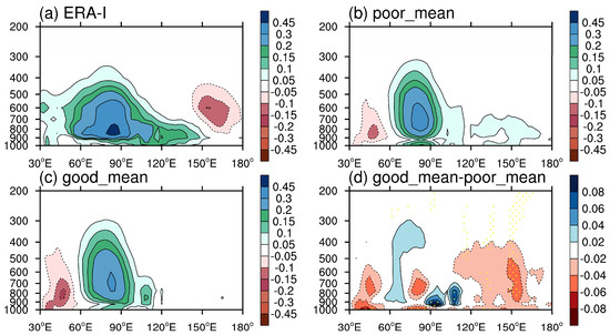
Figure 13.
Longitude-height cross section of regressed specific humidity (averaged over 10° S–10° N) on lag day 0 against the area-averaged 20–100 day filtered OLR time series at the reference area (5° S–5° N; 75°–85° E) in (a) observation, (b) composite of poor simulations, (c) composite of good simulations and (d) difference between composites of good and poor simulations where the differences reaching 90% confidence level are dotted
In order to clarify the dominant source of the pre-moistening, we use the following equation [86]:
where denotes the horizontal velocity vector, is the horizontal gradient operator, is the atmospheric apparent moisture sink, indicates the column integration from surface to 100 hPa. The superscript prime denotes the anomaly regressed against the area-averaged time series of 20–100 day filtered OLR in the reference area (5° S–5° N; 75°–85° E). The first term on the right-hand side of Equation (1) is the horizontal moisture advection. The second term is the large-scale adiabatic vertical motion and the third term represents the subgrid-scale evaporation and condensation. The sum of the second and third terms represents the net moistening associated with the column process. Following Yanai et al. [86], the net moistening associated with the subgrid-scale process can be approximated as the residual term between the moisture tendency and the adiabatic advective processes.
According to Figure 13d, the enhancement of pre-moistening in good simulations is mainly over equatorial MC area (10° S–10° N; 90°–120° E) so that the column-integrated moisture budget terms are averaged over this area. Figure 14 shows the result of such budget analysis in observation, good simulations and poor simulations. Both the tendency terms in observation and composite of good simulations are positive, indicating the accumulation of moisture over this area. But the tendency term in the composite of poor simulations is negative, which accounts for the non-propagating MJO convections. In observation, the positive tendency term over pre-moistening area is mainly contributed by the meridional advection term and the column process while in good and poor simulations, the tendency term is mainly determined by the column process, which is also the most contractive term between good and poor simulations.
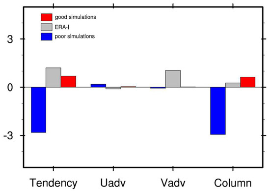
Figure 14.
Results of the regressed moisture budget analysis in observation, good and poor simulations. Four terms presented are defined in Yanai et al. [86]. Each term is regressed against the time series of area-averaged 20–100 day filtered OLR in the reference area (5° S–5° N; 75°–85° E) and then vertically integrated from surface to 100 hPa. The integrated four terms are averaged in the pre-moistening area (10° S–10° N; 90°–120° E) in observation, good and poor simulations.
Therefore, to investigate the role of multi-cloud structure related with convections in pre-moistening, the in Equation (1) is lag regressed from day −20 to 20 against the area-averaged time series of 20–100 day filtered OLR in the reference area (5° S–5° N; 75°–85° E). The four-dimensional is then area-averaged over equatorial MC (10° S–10° N; 90°–120° E) to get the time-height cross section. Results in observation, composite of good simulations, composite of poor simulations are given in Figure 15. In observation, the low-level heating indicating the formation of low-level clouds starts since day −5, destabilizing the atmosphere column, favorable for the following development of shallow convection. Such destabilization and convection development are significantly weakened in poor simulations as the low-level heating starts since day −2 with the heating center higher than that in observation. The heating profile center remains in the low-troposphere after day 0 in observation while both shallow and deep heating sources are found in poor simulations. The difference of profiles between good and poor simulations shows a low-level heating and middle-level cooling from day −5 to day 5, which destabilizes the atmosphere ahead of the MJO major convection, favorable for the development of leading shallow convection. The contrast between profiles indicates a probable enhancement of leading shallow convection.
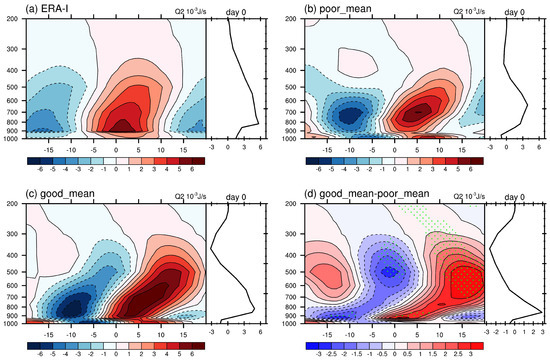
Figure 15.
Time-height cross section (averaged over 10° S–10° N, 90° E–120° E) of lag regressed from day −20 to 20 against the area-averaged 20–100 day filtered OLR time series at the reference area (5° S–5° N; 75°–85° E), along with the regressed profile at day 0 in (a) observation, (b) composite of poor simulations, (c) composite of good simulations and (d) difference between composites of good and poor simulations where the differences reaching 90% confidence level are dotted.
5.2. Key Role of Shallow Convection Leading the Deep Convection
In order to check the enhancement of shallowing convection leading the deep convection of MJO, diagnostics of boundary layer moisture convergence (shown in Figure 16) are conducted. In observation (Figure 16a), strong moisture convergence occurs over the MC when the convective center is over the Indian ocean, indicating the existence of shallow convection leading the updrafts. This leading boundary layer moisture convergence is greatly weakened in the composite of poor simulations, while strong moisture convergence still exists in good simulations. The difference of boundary layer moisture convergence proves that the shallow convection leading MJO major convection in good simulations is indeed enhanced. The enhancement of leading boundary layer moisture convergence also indicates that the BL frictional moisture feedback [87,88] contributes to the improvement of MJO simulation.
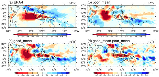
Figure 16.
MJO-related boundary layer moisture convergence which is computed by regressing the vertically integrated (from surface to 700 hPa) moisture convergence against the area-averaged time series of 20–100 day filtered OLR in the reference area (5° S–5° N; 75°–85° E) in (a) observation, (b) composite of poor simulations, (c) composite of good simulations and (d) difference between the composites of good and poor simulations where the differences reaching 90% confidence level are dotted.
To better understand the role of leading shallow convection in better simulation of MJO, regressed structure of apparent heating source () as defined in Yanai et al. [86] is given in Figure 17, along with the regressed profile of equivalent potential temperature (EPT). The regressed structure of in observation shows that the shallow convection heating is triggered a few days before the development of the following deep convection. However, the heating of leading shallow convection vanishes in poor simulations, and the following high-level heating of deep convection is also weakened. The difference of diabatic heating between good and poor simulations shows an enhanced low-level heating caused by shallow convection from day −15. The enhanced leading shallow convection destabilizes the atmosphere column and then develops into deep convection of MJO from lag day 5 to lag day 10. The difference of regressed EPT profile at day 0 between good and poor simulations shows an increase beneath 500 hPa, producing instability for convection to develop. However, the magnitude of such increase is small compared with that of its profile in poor simulations.
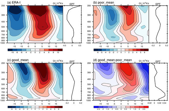
Figure 17.
Time-height cross section (averaged over 10° S–10° N, 90° E–120° E) of lag regressed from day −20 to 20 against the area-averaged 20–100 day filtered OLR time series at the reference area (5° S–5° N; 75°–85° E), along with the regressed equivalent potential temperature profile at day 0 in (a) observation, (b) composite of poor simulations, (c) composite of good simulations and (d) difference between composites of good and poor simulations where the differences reaching 90% confidence level are dotted.
Therefore, the improvement of the pre-moistening effect of MJO is probably due to the enhancement of its leading shallow convection. The deep convective precipitation in poor simulations consumes too much environmental moisture, the light precipitation thus develops in a dryer atmosphere as Figure 12a shows. As a result, the shallow convection precipitation, is insufficient in poor simulations. The shallow convection leading the major convection of MJO is also weakened in poor simulations, which is against its eastward propagation. This is remedied by enhancing the evaporation of deep convective precipitation in good simulations. Meanwhile, the weakened moisture consumption efficiency of shallow convection retains more low-level moisture in good simulations. The improvement of moisture profile in good simulations benefits from both aforementioned effects. The middle-level cooling caused by enhancing the evaporation of deep convection precipitation and the low-level heating caused by strengthening shallow convection destabilize the atmosphere column, favorable for the development of MJO convection and its further propagation.
6. Summary and Discussion
This study analyzed the outputs of 85 model runs produced by perturbing seven chosen parameters in the cloud and convection parameterization schemes of BCC_CSM1.2. Three canonical metrics were used individually to examine each run’s ability of simulating realistic MJO. However, the scoring results of the three metrics do not corroborate each other in our study. Therefore, a new strategy combining the scores of both Lag-correlation and E/W ratio has been used to identify six good and eight poor simulations out of 85 runs. Among the seven chosen parameters as adjustment time scale for shallow convection, relative humidity threshold for high stable clouds, relative humidity threshold for convective trigger, precipitation efficiency for deep convection, precipitation efficiency for shallow convection, relative humidity threshold for low stable clouds and evaporation efficiency for deep convective precipitation, the values of last three parameters showed large differences between good and poor simulations while the rest were almost the same.
MJO exhibits a greater amplitude with an improved eastward propagation in good simulations. Other CCEWs like Kelvin waves are also improved in amplitude and space time structure as Figure 11 shows, consistent with the results of previous research [76]. MJO in poor simulations propagates with a westward speed over India Ocean. Meanwhile, its propagation range over Pacific Ocean shrinks significantly compared with that in observation. After changing values of the abovementioned seven parameters, MJO shows a systematic eastward propagation over India and Pacific Ocean.
The mean state changes along with MJO after parameter perturbation. In poor simulations, excessive precipitation exists in southwest Pacific while insufficient precipitation is produced over MC. The winter mean precipitation gets improved over MC in good simulations by amplifying land rainfalls accompanied with the improvement of MJO propagation. This is consistent to the finding in Peatman et al. [89] that land rainfall is favorable for MJO to cross MC. However, controversy still exists about this conclusion as Zhang and Ling [71] concluded that MJO crosses MC mainly through rainfall over sea. The enhancement of land rainfall over MC, which is dominant by shallow convective precipitation, also indicates changes in the frequency distribution of rain rate. The tropical precipitation consists of too much heavy rainfall in poor simulations as Figure 11a shows. As a result, the environmental atmosphere experiences an overall dry bias in poor simulations since heavy precipitation consumes too much moisture. The dry environmental atmosphere suppresses the frequency of light rainfall. This bias gets improved in good simulations where the frequency distribution of tropical precipitation in Indo-Pacific region is closer to observation by weakening heavy precipitation and increasing the ratio of extremely light rainfall, indicating an enhancement of shallow convection.
The shallow convection leading the deep convection in MJO was enhanced by changing values of three crucial parameters as precipitation efficiency for shallow convection (), relative humidity threshold for low stable clouds () and evaporation efficiency for deep convective precipitation (). shows greater value while values of and are smaller in good simulations. The remaining four parameter values are almost the same as those in poor simulations (Figure 6). Increasing the value of weakens the deep convection precipitation and humidifies the environmental atmosphere. As a result, shallow convection leading the MJO major convection is enhanced, which is reflected by the strengthened low-level moisture convergence ahead of the MJO major convection (as in Figure 16). The enhanced shallow convection is supposed to pump low level moisture to middle troposphere, thus humidifying middle troposphere and drying the low troposphere. However, decreasing value of and increasing value of both lower the low-level moisture consumption efficiency of shallow convection. The whole column of atmosphere is thus humidified with a humidification center at low troposphere. Therefore, the pre-moistening effect over lower-layer atmosphere is also strengthened along with the enhancement of leading shallow convection. Such enhancement of leading shallow convection in good simulations is the key for better simulated MJO. The low-level heating and moistening caused by enhanced shallow convection a few days before the initiation of MJO major convection destabilize the atmosphere column. The leading shallow convection therefore develops to the MJO major deep convection as Figure 17 shows, amplifying the simulated MJO convection. The leading shallow convection also improves the vertical structure of MJO moisture as indicated by Figure 13 and Figure 14, favorable for MJO’s systematic eastward propagation. Boyle et. al. [90] conducted a similar parameter perturbation experiment with CAM5, but they perturbed more parameters in not only cloud and convection parameterization schemes, but also in radiation, boundary layer and turbulence parameterizations. They showed that the MJO simulation also displayed a strong sensitivity to the parameter associated with the deep convection. They also demonstrated that by changing deep convection parameter values to suppress deep convective precipitation, MJO simulation is improved. This is consistent with the conclusion of this study. Other mechanisms such as the atmosphere-ocean interaction may also contribute to the improvement of the MJO simulation as Figure 7 shows that SST in good simulations shows an overall warming over Indian ocean which could excite more MJO events. Besides, the rise of SST in east Pacific exhibits an El Niño-like pattern, which is favorable for MJO’s eastward propagation.
This work is an attempt to reveal the important parameter-related physical processes for simulating realistic MJO in BCC_CSM1.2, hoping to provide inspirations for the simulation and prediction of MJO. Three parameters were found different largely in good and poor simulations. By changing the values of these three parameters, the moisture sensitivity of convection becomes different, leading to an enhanced leading shallow convection, accounting for the improvement of MJO. However, some aspects of this research still need further study. Even integrations with relatively high-skill MJO simulations show deficiencies of simulating realistic MJO as most MJO related figures in good simulations also show considerable differences compared with observation. This is likely because we only perturbed the parameter values without changing any other components in the model, so the model’s systematic deficiencies in simulating MJO [91] may not be totally compensated. However, composite results of good simulations all exhibit changes for a better simulated MJO, proving the validity of such certain parameter perturbation. But detailed physical processes in cloud dynamics and convections determining the improvement of MJO still remains unrevealed, which needs further related studies.
Author Contributions
Conceptualization, K.H. and H.-L.R.; Data curation, X.L.; Supervision, H.-L.R. and M.M.; Validation, K.H.; Writing—original draft preparation, K.H.; Writing—review and editing, H.-L.R., P.R., and Y.W.
Funding
This work was jointly supported by the National Key Research and Development Program on monitoring, Early Warning and Prevention of Major Natural Disaster (2017YFC1502302, 2018YFC1505906), State Oceanic Administration International Cooperation Program (GASI-IPOVAI-03), China National Science Foundation project (41606019), and China Meteorological Administration Special Public Welfare Research Fund (GYHY201506013).
Acknowledgments
The authors gratefully acknowledge Fei-Fei Jin, Joshua-Xiouhua Fu, Wansuo Duan, Guodong Sun, Fei Liu, Yujie Wu and Ming Bao for their kindly discussions about this work. Constructive comments by three anonymous reviewers led to substantial improvements in the presentation. ERA-interim Reanalysis data was provided by the ECMWF from their Web site at https://www.ecmwf.int/en/forecasts/datasets/reanalysis-datasets/era-interim. Daily interpolated OLRs were obtained from NOAA/OAR/ESRL PSD, Boulder, Colorado, USA https://www.esrl.noaa.gov/psd/data/gridded/data.interp_OLR.html.
Conflicts of Interest
The authors declare no conflict of interest.
References
- Madden, R.A.; Julian, P.R. Detection of a 40–50 day oscillation in the zonal wind in the tropical Pacific. J. Atmos. Sci. 1971, 28, 702–708. [Google Scholar] [CrossRef]
- Madden, R.A.; Julian, P.R. Description of global-scale circulation cells in the tropics with a 40–50 day period. J. Atmos. Sci. 1972, 29, 1109–1123. [Google Scholar] [CrossRef]
- Lau, W.K.-M.; Waliser, D.E. Intraseasonal Variability in the Atmosphere-Ocean Climate System; Springer Science & Business Media: Berlin, Germany, 2011. [Google Scholar]
- Zhang, C.D. Madden-Julian oscillation. Rev. Geophys. 2005, 43, 36. [Google Scholar] [CrossRef]
- Wei, Y.; Liu, F.; Mu, M.; Ren, H.-L. Planetary scale selection of the Madden–Julian Oscillation in an air-sea coupled dynamic moisture model. Clim Dyn. 2017, 50, 3441–3456. [Google Scholar] [CrossRef]
- Zhang, C. Madden–Julian oscillation: Bridging Weather and Climate. Bull. Am. Meteorol. Soc. 2013, 94. [Google Scholar] [CrossRef]
- Kim, H.-K.; Seo, K.-H. Cluster analysis of tropical cyclone tracks over the western north pacific using a self-organizing map. J. Clim. 2016, 29, 3731–3751. [Google Scholar] [CrossRef]
- Adames, A.F.; Wallace, J.M. Three-Dimensional Structure and Evolution of the Vertical Velocity and Divergence Fields in the MJO. J. Atmos. Sci. 2014, 71, 267–287. [Google Scholar] [CrossRef]
- Weickmann, K.M. Intraseasonal circulation and outgoing longwave radiation modes during Northern Hemisphere winter. Mon. Weather Rev. 1983, 111, 1838–1858. [Google Scholar] [CrossRef]
- Wang, B.; Liu, F.; Chen, G. A trio-interaction theory for Madden–Julian oscillation. Geosci. Lett. 2016, 3, 34. [Google Scholar] [CrossRef]
- Wang, B.; Rui, H. Dynamics of the coupled moist Kelvin–Rossby wave on an equatorial β-plane. J. Atmos. Sci. 1990, 47, 397–413. [Google Scholar] [CrossRef]
- Liu, F.; Wang, B. Roles of the moisture and wave feedbacks in shaping the Madden–Julian oscillation. J. Clim. 2017, 30, 10275–10291. [Google Scholar] [CrossRef]
- Adames, Á.F.; Kim, D. The MJO as a dispersive, convectively coupled moisture wave: Theory and observations. J. Atmos. Sci. 2016, 73, 913–941. [Google Scholar] [CrossRef]
- Sobel, A.; Maloney, E. An idealized semi-empirical framework for modeling the Madden–Julian oscillation. J. Atmos. Sci. 2012, 69, 1691–1705. [Google Scholar] [CrossRef]
- Sobel, A.; Maloney, E. Moisture modes and the eastward propagation of the MJO. J. Atmos. Sci. 2013, 70, 187–192. [Google Scholar] [CrossRef]
- Woolnough, S.; Slingo, J.; Hoskins, B. The organization of tropical convection by intraseasonal sea surface temperature anomalies. Q. J. R. Meteorol. Soc. 2001, 127, 887–907. [Google Scholar] [CrossRef]
- Andersen, J.A.; Kuang, Z. Moist static energy budget of MJO-like disturbances in the atmosphere of a zonally symmetric aquaplanet. J. Clim. 2012, 25, 2782–2804. [Google Scholar] [CrossRef]
- Kim, D.; Kug, J.-S.; Sobel, A.H. Propagating versus nonpropagating Madden–Julian oscillation events. J. Clim. 2014, 27, 111–125. [Google Scholar] [CrossRef]
- Maloney, E.D. The moist static energy budget of a composite tropical intraseasonal oscillation in a climate model. J. Clim. 2009, 22, 711–729. [Google Scholar] [CrossRef]
- Maloney, E.D.; Sobel, A.H.; Hannah, W.M. Intraseasonal variability in an aquaplanet general circulation model. J. Adv. Model. Earth Syst. 2010, 2. [Google Scholar] [CrossRef]
- Liu, F.; Wang, B. Effects of moisture feedback in a frictional coupled Kelvin–Rossby wave model and implication in the Madden–Julian oscillation dynamics. Clim. Dyn. 2017, 48, 513–522. [Google Scholar] [CrossRef]
- Wang, B.; Chen, G. A general theoretical framework for understanding essential dynamics of Madden–Julian oscillation. Clim. Dyn. 2017, 49, 2309–2328. [Google Scholar] [CrossRef]
- Biello, J.A.; Majda, A.J. A new multiscale model for the Madden–Julian oscillation. J. Atmos. Sci. 2005, 62, 1694–1721. [Google Scholar] [CrossRef]
- Liu, F.; Huang, G.; Feng, L. Critical roles of convective momentum transfer in sustaining the multi-scale Madden–Julian oscillation. Theor. Appl. Climatol. 2012, 108, 471–477. [Google Scholar] [CrossRef]
- Liu, F.; Wang, B. A frictional skeleton model for the Madden–Julian oscillation. J. Atmos. Sci. 2012, 69, 2749–2758. [Google Scholar] [CrossRef]
- Liu, F.; Wang, B. A model for the interaction between 2-day waves and moist Kelvin waves. J. Atmos. Sci. 2012, 69, 611–625. [Google Scholar] [CrossRef]
- Majda, A.J.; Biello, J.A. A multiscale model for tropical intraseasonal oscillations. Proc. Natl. Acad. Sci. USA 2004, 101, 4736–4741. [Google Scholar] [CrossRef] [PubMed]
- Wang, B.; Liu, F. A model for scale interaction in the Madden–Julian oscillation. J. Atmos. Sci. 2011, 68, 2524–2536. [Google Scholar] [CrossRef]
- Khouider, B.; Majda, A.J. A Simple multicloud parameterization for convectively coupled tropical waves. Part I: Linear analysis. J. Atmos. Sci. 2006, 63, 1308–1323. [Google Scholar] [CrossRef]
- Khouider, B.; Majda, A.J. A simple multicloud parameterization for convectively coupled tropical waves. Part II: Nonlinear simulations. J. Atmos. Sci. 2007, 64, 381–400. [Google Scholar] [CrossRef]
- Yang, D.; Ingersoll, A.P. Testing the hypothesis that the MJO is a mixed Rossby–gravity wave packet. J. Atmos. Sci. 2011, 68, 226–239. [Google Scholar] [CrossRef]
- Yang, D.; Ingersoll, A.P. Triggered convection, gravity waves, and the MJO: A shallow-water model. J. Atmos. Sci. 2013, 70, 2478–2486. [Google Scholar] [CrossRef]
- Yang, D.; Ingersoll, A.P. A theory of the MJO horizontal scale. Geophys. Res. Lett. 2014, 41, 1059–1064. [Google Scholar] [CrossRef]
- Wang, B.; Xie, X. A Model for the boreal summer intraseasonal oscillation. J. Atmos. Sci. 1997, 54, 72–86. [Google Scholar] [CrossRef]
- Fu, X.; Wang, B. The Boreal-Summer intraseasonal oscillations simulated in a hybrid coupled atmosphere–ocean model. Mon. Weather Rev. 2004, 132, 2628–2649. [Google Scholar] [CrossRef]
- Liu, F.; Wang, B. An air–sea coupled skeleton model for the Madden–Julian oscillation. J. Atmos. Sci. 2013, 70, 3147–3156. [Google Scholar] [CrossRef]
- Wang, B.; Xie, X. Coupled modes of the warm pool climate system. Part I: The role of air–sea interaction in maintaining Madden–Julian oscillation. J. Clim. 1998, 11, 2116–2135. [Google Scholar] [CrossRef]
- Cao, G.; Zhang, G.J. Role of Vertical Structure of Convective Heating in MJO Simulation in NCAR CAM5.3. J. Clim. 2017, 30, 7423–7439. [Google Scholar] [CrossRef]
- Fu, X.H.; Lee, J.Y.; Hsu, P.C.; Taniguchi, H.; Wang, B.; Wang, W.Q.; Weaver, S. Multi-model MJO forecasting during DYNAMO/CINDY period. Clim. Dyn. 2013, 41, 1067–1081. [Google Scholar] [CrossRef][Green Version]
- Fu, X.H.; Lee, J.Y.; Wang, B.; Wang, W.Q.; Vitart, F. Intraseasonal Forecasting of the Asian Summer Monsoon in Four Operational and Research Models. J. Clim. 2013, 26, 4186–4203. [Google Scholar] [CrossRef]
- Jiang, X.; Waliser, D.E.; Xavier, P.K.; Petch, J.; Klingaman, N.P.; Woolnough, S.J.; Guan, B.; Bellon, G.; Crueger, T.; DeMott, C.; et al. Vertical structure and physical processes of the Madden-Julian oscillation: Exploring key model physics in climate simulations. J. Geophys. Res. Atmos. 2015, 120, 4718–4748. [Google Scholar] [CrossRef]
- Ling, J.; Zhang, C.; Wang, S.; Li, C. A new interpretation of the ability of global models to simulate the MJO. Geophys. Res. Lett. 2017, 44, 5798–5806. [Google Scholar] [CrossRef]
- Xavier, P.K.; Petch, J.C.; Klingaman, N.P.; Woolnough, S.J.; Jiang, X.A.; Waliser, D.E.; Caian, M.; Cole, J.; Hagos, S.M.; Hannay, C.; et al. Vertical structure and physical processes of the Madden-Julian Oscillation: Biases and uncertainties at short range. J. Geophys. Res. Atmos. 2015, 120, 4749–4763. [Google Scholar] [CrossRef] [PubMed]
- Hung, M.-P.; Lin, J.-L.; Wang, W.; Kim, D.; Shinoda, T.; Weaver, S.J. MJO and convectively coupled equatorial waves simulated by CMIP5 climate models. J. Clim. 2013, 26, 6185–6214. [Google Scholar] [CrossRef]
- Waliser, D.; Sperber, K.; Hendon, H.; Kim, D.; Wheeler, M.; Weickmann, K.; Zhang, C.; Donner, L.; Gottschalck, J.; Higgins, W.; et al. MJO Simulation Diagnostics. J. Clim. 2009, 22, 3006–3030. [Google Scholar]
- Wheeler, M.C.; Hendon, H.H. An all-season real-time multivariate MJO index: development of an Index for monitoring and prediction. Mon Weather Rev. 2004, 132. [Google Scholar] [CrossRef]
- Tiedtke, M. A Comprehensive Mass Flux Scheme for Cumulus Parameterization in Large-Scale Models. Mon Weather Rev. 1989, 117, 1779–1800. [Google Scholar] [CrossRef]
- Zhang, G.J.; McFarlane, N.A. Sensitivity of climate simulations to the parameterization of cumulus convection in the Canadian climate centre general circulation model. Atmos. Ocean. 1995, 33, 407–446. [Google Scholar] [CrossRef]
- Zhang, G.J.; Mu, M. Effects of modifications to the Zhang-McFarlane convection parameterization on the simulation of the tropical precipitation in the National Center for Atmospheric Research Community Climate Model, version 3. J. Geophys. Res. Atmos. 2005, 110. [Google Scholar] [CrossRef]
- Tokioka, T.; Yamazaki, K.; Kitoh, A.; Ose, T. The equatorial 30–60 day oscillation and the Arakawa-Schubert penetrative cumulus parameterization. J. Meteorol. Soc. Jpn. Ser. II 1988, 66, 883–901. [Google Scholar] [CrossRef]
- Wang, W.; Schlesinger, M.E. The dependence on convection parameterization of the tropical intraseasonal oscillation simulated by the UIUC 11-layer atmospheric GCM. J. Clim. 1999, 12, 1423–1457. [Google Scholar] [CrossRef]
- Maloney, E.D.; Hartmann, D.L. The sensitivity of intraseasonal variability in the NCAR CCM3 to changes in convective parameterization. J. Clim. 2001, 14, 2015–2034. [Google Scholar] [CrossRef]
- Fu, X.; Wang, B. Critical roles of the stratiform rainfall in sustaining the Madden–Julian oscillation: GCM experiments. J. Clim. 2009, 22, 3939–3959. [Google Scholar] [CrossRef]
- Bretherton, C.S.; Peters, M.E.; Back, L.E. Relationships between water vapor path and precipitation over the tropical oceans. J. Clim. 2004, 17, 1517–1528. [Google Scholar] [CrossRef]
- Kim, D.; Xavier, P.; Maloney, E.; Wheeler, M.; Waliser, D.; Sperber, K.; Hendon, H.; Zhang, C.; Neale, R.; Hwang, Y.-T. Process-oriented MJO simulation diagnostic: Moisture sensitivity of simulated convection. J. Clim. 2014, 27, 5379–5395. [Google Scholar] [CrossRef]
- Thayer-Calder, K.; Randall, D.A. The Role of Convective Moistening in the Madden-Julian Oscillation. J. Atmos. Sci. 2009, 66, 3297–3312. [Google Scholar] [CrossRef]
- Liu, X.; Li, W.; Wu, T.; Li, T.; Gu, W.; Bo, Z.; Yang, B.; Zhang, L.; Jie, W. Validity of parameter optimization in improving MJO simulation and prediction using the sub-seasonal to seasonal forecast model of Beijing Climate Center. Clim Dyn. 2018, 52, 3823–3843. [Google Scholar] [CrossRef]
- Wu, T.; Song, L.; Li, W.; Wang, Z.; Zhang, H.; Xin, X.; Zhang, Y.; Zhang, L.; Li, J.; Wu, F.; et al. An overview of BCC climate system model development and application for climate change studies. J. Meteorol. Res. 2014, 28, 34–56. [Google Scholar] [CrossRef]
- Ji, J.; Huang, M.; Li, K. Prediction of carbon exchanges between China terrestrial ecosystem and atmosphere in 21st century. Sci. China Ser. D Earth Sci. 2008, 51, 885–898. [Google Scholar] [CrossRef]
- Winton, M. A Reformulated Three-Layer Sea Ice Model. J. Atmos. Ocean. Technol. 2000, 17, 525–531. [Google Scholar] [CrossRef]
- Wu, T.; Yu, R.; Zhang, F.; Wang, Z.; Dong, M.; Wang, L.; Jin, X.; Chen, D.; Li, L. The Beijing Climate Center atmospheric general circulation model: description and its performance for the present-day climate. Clim Dyn. 2008, 34, 123. [Google Scholar] [CrossRef]
- McKay, M.D. Latin hypercube sampling as a tool in uncertainty analysis of computer models. In Proceedings of the 24th Conference on Winter Simulation, Arlington, VA, USA, 13–16 December 1992; ACM Press: New York, NY, USA, 1947; pp. 557–564. [Google Scholar]
- Liebmann, B.; Smith, C.A. Description of a Complete (Interpolated) Outgoing Longwave Radiation Dataset. Bull. Am. Meteorol. Soc. 1996, 77, 1275–1277. [Google Scholar]
- Huffman, G.J.; Bolvin, D.T.; Nelkin, E.J.; Wolff, D.B.; Adler, R.F.; Gu, G.; Hong, Y.; Bowman, K.P.; Stocker, E.F. The TRMM Multisatellite Precipitation Analysis (TMPA): Quasi-Global, Multiyear, Combined-Sensor Precipitation Estimates at Fine Scales. J. Hydrometeorol. 2007, 8, 38–55. [Google Scholar] [CrossRef]
- Dee, D.P.; Uppala, S.M.; Simmons, A.J.; Berrisford, P.; Poli, P.; Kobayashi, S.; Andrae, U.; Balmaseda, M.A.; Balsamo, G.; Bauer, P.; et al. The ERA-Interim reanalysis: Configuration and performance of the data assimilation system. Q. J. R. Meteorol. Soc. 2011, 137, 553–597. [Google Scholar] [CrossRef]
- Hannah, W.M.; Maloney, E.D. The Role of Moisture-Convection Feedbacks in Simulating the Madden-Julian Oscillation. J. Clim. 2011, 24, 2754–2770. [Google Scholar] [CrossRef]
- Hirota, N.; Ogura, T.; Tatebe, H.; Shiogama, H.; Kimoto, M.; Watanabe, M. Roles of Shallow Convective Moistening in the Eastward Propagation of the MJO in MIROC6. J. Clim. 2018, 31, 3033–3047. [Google Scholar] [CrossRef]
- Maloney, E.D.; Wolding, B.O. Initiation of an intraseasonal oscillation in an aquaplanet general circulation model. J. Adv. Model. Earth Syst. 2015, 7, 1956–1976. [Google Scholar] [CrossRef]
- Wolding, B.O.; Maloney, E.D. Objective Diagnostics and the Madden–Julian Oscillation. Part I: Methodology. J. Clim. 2015, 28, 4127–4140. [Google Scholar] [CrossRef]
- Wheeler, M.; Kiladis, G.N. Convectively coupled equatorial waves: Analysis of clouds and temperature in the wavenumber-frequency domain. J. Atmos. Sci. 1999, 56, 374–399. [Google Scholar] [CrossRef]
- Zhang, C.D.; Ling, J. Barrier Effect of the Indo-Pacific Maritime Continent on the MJO: Perspectives from Tracking MJO Precipitation. J. Clim. 2017, 30, 3439–3459. [Google Scholar] [CrossRef]
- Zhang, Y.; Xie, S.; Covey, C.; Lucas, D.D.; Gleckler, P.; Klein, S.A.; Tannahill, J.; Doutriaux, C.; Klein, R. Regional assessment of the parameter-dependent performance of CAM4 in simulating tropical clouds. Geophys. Res. Lett. 2012, 39, L14708. [Google Scholar] [CrossRef]
- Yoneyama, K.; Zhang, C.; Long, C.N. Tracking pulses of the Madden–Julian oscillation. Bull. Am. Meteorol. Soc. 2013, 94, 1871–1891. [Google Scholar] [CrossRef]
- Wei, Y.; Mu, M.; Ren, H.L.; Fu, J.X. Conditional Nonlinear Optimal Perturbations of Moisture Triggering Primary MJO Initiation. Geophys. Res. Lett. 2019, 46, 3492–3501. [Google Scholar] [CrossRef]
- Guo, Y.; Jiang, X.; Waliser, D.E. Modulation of the convectively coupled Kelvin waves over South America and the tropical Atlantic Ocean in association with the Madden–Julian oscillation. J. Atmos. Sci. 2014, 71, 1371–1388. [Google Scholar] [CrossRef]
- Guo, Y.; Waliser, D.E.; Jiang, X. A Systematic Relationship between the Representations of Convectively Coupled Equatorial Wave Activity and the Madden–Julian Oscillation in Climate Model Simulations. J. Clim. 2015, 28, 1881–1904. [Google Scholar] [CrossRef]
- Kim, D.; Sperber, K.; Stern, W.; Waliser, D.; Kang, I.-S.; Maloney, E.; Wang, W.; Weickmann, K.; Benedict, J.; Khairoutdinov, M. Application of MJO simulation diagnostics to climate models. J. Clim. 2009, 22, 6413–6436. [Google Scholar] [CrossRef]
- Chang, C.W.J.; Tseng, W.L.; Hsu, H.H.; Keenlyside, N.; Tsuang, B.J. The Madden-Julian Oscillation in a warmer world. Geophys. Res. Lett. 2015, 42, 6034–6042. [Google Scholar] [CrossRef]
- Maloney, E.D.; Adames, Á.F.; Bui, H.X. Madden–Julian oscillation changes under anthropogenic warming. Nat. Clim. Chang. 2019, 9, 26–33. [Google Scholar] [CrossRef]
- Gonzalez, A.O.; Jiang, X. Winter mean lower tropospheric moisture over the Maritime Continent as a climate model diagnostic metric for the propagation of the Madden-Julian oscillation. Geophys. Res. Lett. 2017, 44, 2588–2596. [Google Scholar] [CrossRef]
- Xavier, P.K. Intraseasonal Convective Moistening in CMIP3 Models. J. Clim. 2012, 25, 2569–2577. [Google Scholar] [CrossRef]
- Hsu, P.-C.; Li, T. Role of the boundary layer moisture asymmetry in causing the eastward propagation of the Madden–Julian oscillation. J. Clim 2012, 25, 4917–4931. [Google Scholar] [CrossRef]
- Zhao, C.; Li, T.; Zhou, T. Precursor signals and processes associated with MJO initiation over the tropical Indian Ocean. J. Clim. 2013, 26, 291–307. [Google Scholar] [CrossRef]
- Hsu, P.-C.; Li, T.; Murakami, H. Moisture asymmetry and MJO eastward propagation in an aquaplanet general circulation model. J. Clim. 2014, 27, 8747–8760. [Google Scholar] [CrossRef]
- Wang, L.; Li, T.; Maloney, E.; Wang, B. Fundamental Causes of Propagating and Nonpropagating MJOs in MJOTF/GASS Models. J. Clim. 2017, 30, 3743–3769. [Google Scholar] [CrossRef]
- Yanai, M.; Esbensen, S.; Chu, J.-H. Determination of bulk properties of tropical cloud clusters from large-scale heat and moisture budgets. J. Atmos. Sci. 1973, 30, 611–627. [Google Scholar] [CrossRef]
- Wang, B. Dynamics of tropical low-frequency waves: An analysis of the moist Kelvin wave. J. Atmos. Sci. 1988, 45, 2051–2065. [Google Scholar] [CrossRef]
- Wang, B.; Chen, J. On the zonal-scale selection and vertical structure of equatorial intraseasonal waves. Q. J. R. Meteorol. Soc. 1989, 115, 1301–1323. [Google Scholar] [CrossRef]
- Peatman, S.C.; Matthews, A.J.; Stevens, D.P. Propagation of the Madden–Julian Oscillation through the Maritime Continent and scale interaction with the diurnal cycle of precipitation. Q. J. R. Meteorol. Soc. 2014, 140, 814–825. [Google Scholar] [CrossRef]
- Boyle, J.; Klein, S.; Lucas, D.; Ma, H.Y.; Tannahill, J.; Xie, S. The parametric sensitivity of CAM5’s MJO. J. Geophys. Res. Atmos. 2015, 120, 1424–1444. [Google Scholar] [CrossRef]
- Liu, X.; Wu, T.; Yang, S.; Li, T.; Jie, W.; Zhang, L.; Wang, Z.; Liang, X.; Li, Q.; Cheng, Y. MJO prediction using the sub-seasonal to seasonal forecast model of Beijing Climate Center. Clim Dyn. 2017, 48, 3283–3307. [Google Scholar] [CrossRef]
© 2019 by the authors. Licensee MDPI, Basel, Switzerland. This article is an open access article distributed under the terms and conditions of the Creative Commons Attribution (CC BY) license (http://creativecommons.org/licenses/by/4.0/).