A Study of Objective Prediction for Summer Precipitation Patterns Over Eastern China Based on a Multinomial Logistic Regression Model

Abstract

The prediction of summer precipitation patterns (PPs) over eastern China is an important and topical issue in China. Predictors that are selected based on historical information may not be suitable for the future due to non-stationary relationships between summer precipitations and corresponding predictors, and might induce the instability of prediction models, especially in cases with few predictors. This study aims to investigate how to learn as much information as possible from various and numerous predictors reflecting different climate conditions. An objective prediction method based on the multinomial logistic regression (MLR) model is proposed to facilitate the study. The predictors are objectively selected from a machine learning perspective. The effectiveness of the objective prediction model is assessed by considering the influence of collinearity and number of predictors. The prediction accuracy is found to be comparable to traditionally estimated predictability, ranging between 0.6 and 0.7. The objective prediction model is capable of learning the intrinsic structure of the predictors, and is significantly superior to the prediction model with randomly-selected predictors and the single best predictor. A robust prediction can be generally obtained by learning information from plenty of predictors, although the most effective model may be constructed with fewer predictors through proper methods of predictor selection. In addition, the effectiveness of objective prediction is found to generally improve as observation increases, highlighting its potential for improvement during application as time passes.

1. Introduction

Summer precipitation over eastern China, a region with a densely distributed population and cultivated/industrial lands, is mainly controlled by the East Asian summer monsoon (EASM). The main belt of precipitation advances northward in a step-wise manner with the seasonally-evolving EASM during the summer time. However, various climate factors, with strong inter-annual variability, could lead to complicated regional patterns of precipitation associated with severe floods and droughts in the region [1,2]. For instance, more than four thousand people were killed in the unusually extensive floods in the Yangtze River valleys in 1998, and the direct economic losses were estimated to be over $20 billion. Therefore, prediction of the summer precipitation patterns (PPs) over eastern China has been an important issue for the Chinese government [3]. It helps to determine the focus of flood control and the distribution of disaster-prevention materials. The operational prediction of summer precipitation is routinely made in March by the National Climate Center of China Meteorological Administration (NCC-CMA) to meet the public service. However, although a considerable amount of research has been done on the prediction of summer precipitation in China, with both statistical and dynamical methods, the skill has remained quite limited [4,5,6]. Various efforts have been continually made, but it is still hard to improve the prediction skill [7,8]. The present paper introduces a novel approach to the statistical prediction of summer PPs over eastern China by using machine learning or data-driving methods.

The key to statistical prediction is the selection of skillful predictors. Many studies have shown close relationships between summer precipitation and simultaneous atmospheric circulations and oceanic signals [9,10]. For instance, the western Pacific subtropical high ridge position and western ridge point were found to be well-associated with the location of the main precipitation belt [11,12]; the growing and decaying phases of El Niño and Southern Oscillation (ENSO) corresponding to different PPs in eastern China [13,14,15]. However, precursors (predictors) rather than simultaneous signals are needed to make predictions. Previous studies have found several important preceding winter climate factors, or predictors, such as ENSO [16,17,18], snow cover over the Tibetan Plateau [19,20], the North Atlantic Oscillation [21,22], the North Pacific Oscillation [23], atmospheric circulation patterns over East Asia [24], and sea surface temperature over the Indo-Pacific ocean [25]. Statistical models constructed based on these predictors have played an important role in past operational predictions [23].

The main problem of statistical prediction is that the effectiveness of predictors varies in different periods. For instance, the prediction models in [26] showed a 67% accuracy for the period 1989–2000, while this figure was reduced to 42% for 2001–2012 [27]. This suggests that predictors selected based on physical mechanisms and/or statistical relations from historical records may not be suitable for the future due to non-stationary relationships between the climate (precipitation) and corresponding predictors. There is no perpetual dominant physical process that determines the summer PPs due to the nonlinearity and complexity of the climate system. Consequently, it is very difficult to find any persistently effective predictors, and the prediction models must be reconstructed by selecting new predictors in order to ensure a sufficient accuracy. Therefore, in this study, we propose a systematic approach to the prediction of the summer PPs over eastern China, in which the predictors are objectively selected from a machine learning perspective. This is conducted to extract as much useful information as possible from various predictors representing the relevant atmosphere, ocean, and land surface states, and to establish robust statistical relations between the preceding winter climate conditions and the summer PPs via assessing the effectiveness of the objective prediction model.

In general, summer precipitation over eastern China can be categorized into three typical PPs (Figure 1), which are characterized by different locations of the main rainfall belt [28]. In the first PP, the positive anomalies of precipitation are mainly in the Yellow River valley and to the north. In the second PP, the positive anomalies of precipitation are mainly in the Huai River valley, between the Yellow River and the Yangtze River. In the third PP, the positive anomalies are mainly in the Yangtze River valley and to the south. For each summer, a specific PP category is empirically designated by NCC-CMA according to similarity with the real precipitation pattern. The three PPs generally correspond to different climate conditions and are dominated by quite distinct large-scale atmospheric circulation patterns. They are efficient and convenient in depicting summer precipitation over eastern China, and have often been used as indicators in many studies [2,29], particularly in the operational prediction of summer precipitation by NCC-CMA. It is worth noting that three indicators are well-suited for machine learning classification methods. Previous predictive studies on PPs were usually based on simple conceptual models, in which the parameters were subjectively designated [27]. In the present study, the PPs are directly determined by predictors and the parameters are iteratively learned from the machine learning classification model.

The multinomial logistic regression (MLR) model, known as a generalized linear classification model, is used to classify PPs [30]. Nonlinear methods are more powerful in fitting data, but they may not have advantages in dealing with short climate data because of the overfitting problem and are not involved in this study. The generalization ability of the objective prediction model is assessed in this study considering the small sample size and non-stationarity of the climate system. The article is organized as follows: the data and the machine learning method are described in Section 2; the procedures of the objective selection of predictors are introduced in Section 3; the results of training, validation, the generalization abilities of the model are analyzed in Section 4; and the main conclusions of the study are summarized in Section 5.

2. Data and Machine Learning Method

2.1. Data

The predictors are mainly taken from a monthly climate indices dataset provided by NCC-CMA (https://cmdp.ncc-cma.net/en). This dataset contains 88 atmospheric circulation indices, 26 sea surface temperature indices, and 16 other climate indices (available from https://cmdp.ncc-cma.net/Monitoring/cn_index_130.php). These 130 indices are not necessarily produced with the aim of predicting summer PPs over eastern China, but involve plenty of climate factors that reflect the global climate. An additional climate index calculated by averaging the snow depth of weather stations over the Qinghai-Tibetan Plateau is used as one of the potential predictors mentioned in the Introduction section. The median values of indices in the preceding December, and current January and February are selected to represent corresponding winter states. It should be noted that spring indices usually have less correlation with summer PPs than those of the preceding winter due to transitivity of the spring season [31]. The years of three PPs defined by NCC-CMA are shown in

Table 1. Classifications of summer precipitation pattern over eastern China from 1952–2012.

Class	Year
I	1953 1958 1959 1960 1961 1964 1966 1967 1973 1976 1977 1978 1981 1985 1988 1992 1994 1995 2004 2012
II	1956 1957 1962 1963 1965 1971 1972 1975 1979 1982 1984 1987 1989 1990 1991 2000 2003 2005 2007 2008 2009
III	1952 1954 1955 1968 1969 1970 1974 1980 1983 1986 1993 1996 1997 1998 1999 2001 2002 2006 2010 2011

. The frequencies of the three PPs are close, with 20, 21, and 20 years, respectively, in the study period. The analyses are performed for the period of 1952–2012, for which all the data are available. Predictors with any missing values or too many equal values are removed and 84 predictors are preliminarily selected (details in Appendix A).

2.2. Multinomial Logistic Regression

The MLR model is a basic classification machine learning method for multi-class studies [30]. It is a generalization of the logistic regression model [32]. For a training set of m samples with k classes:

$$\left\{\left(x^{\left(1\right)},y^{\left(1\right)}\right),\dots ,\left(x^{\left(i\right)},y^{\left(i\right)}\right),\dots ,\left(x^{\left(m\right)},y^{\left(m\right)}\right)\right\},$$

the posterior probabilities are given by a normalized exponential form (also known as the softmax function):

$$\mathrm{p}\left(y^{\left(i\right)}=l|x^{\left(i\right)},w\right)=\frac{e^{w_l^T{x}^{\left(i\right)}}}{{{\displaystyle \sum }}_{l=1}^k{e}^{w_l^T{x}^{\left(i\right)}}}$$

where ${\mathrm{x}}^{\left(\mathrm{i}\right)}$ denotes the $i\mathrm{th}$ input feature vectors (i.e., predictors) with $n$ dimension, $y^{\left(i\right)}$ denotes the label of $\mathrm{ith}$ samples, and $\mathrm{w}$ denotes the parameter of the model. The hypothesis function gives the probability of a sample $x^i$ belonging to class $l$. The optimum parameter $w$ can be obtained by maximizing the likelihood function, which is equivalent to minimizing the cost function based on the logarithmic likelihood function:

$$\begin{array}{l}J\left(w\right)=-\ln \left(\frac{1}{m}{\displaystyle \prod }_{i=1}^m{\displaystyle \prod }_{l=1}^{k}p\left(y^{\left(i\right)}=l|x^{\left(i\right)},w\right)\right)\\ \hspace{1em}\hspace{1em}\hspace{1em}\hspace{1em}\hspace{1em}=-\frac{1}{m}·{\displaystyle \sum _{i=1}^m}\left({\displaystyle \sum _{l=1}^k}\left(\mu \left(y^{\left(i\right)}=l\right)·\ln \left(\frac{e^{w_l^T{x}^{\left(i\right)}}}{{{\displaystyle \sum }}_{l=1}^k{e}^{w_l^T{x}^{\left(i\right)}}}\right)\right)\right)\end{array}$$

where $\mu$ is the indicator function, so that $\mu \left(y^{\left(i\right)}=l\right)=1$ when $y^{\left(i\right)}=l$ is true and $\mu \left(y^{\left(i\right)}=l\right)=0$ when $y^{\left(i\right)}=l$ is false. An iterative optimization algorithm such as gradient descent can be used to solve the problem and find the minimum of $J\left(w\right)$. To guarantee that the cost function $J\left(w\right)$ is strictly convex, a weight decay penalty term should be added to penalize large values of the parameters. Two popular penalty terms are $\lambda {\displaystyle \sum }_{l=1}^k{\displaystyle \sum }_{j=1}^n{w}_{lj}^2$ and $\lambda {\displaystyle \sum }_{l=1}^k{\displaystyle \sum }_{j=1}^n\left|w_{lj}\right|$, which are known as L2 regularization and L1 regularization, respectively [30]. In this study, the MLR model with L2 regularization is used to classify the three PPs classes. In addition, the MLR model with L1 regularization usually obtains sparse parameters, which means that only parts of features are used in the model.

3. Objective Selection of Predictors

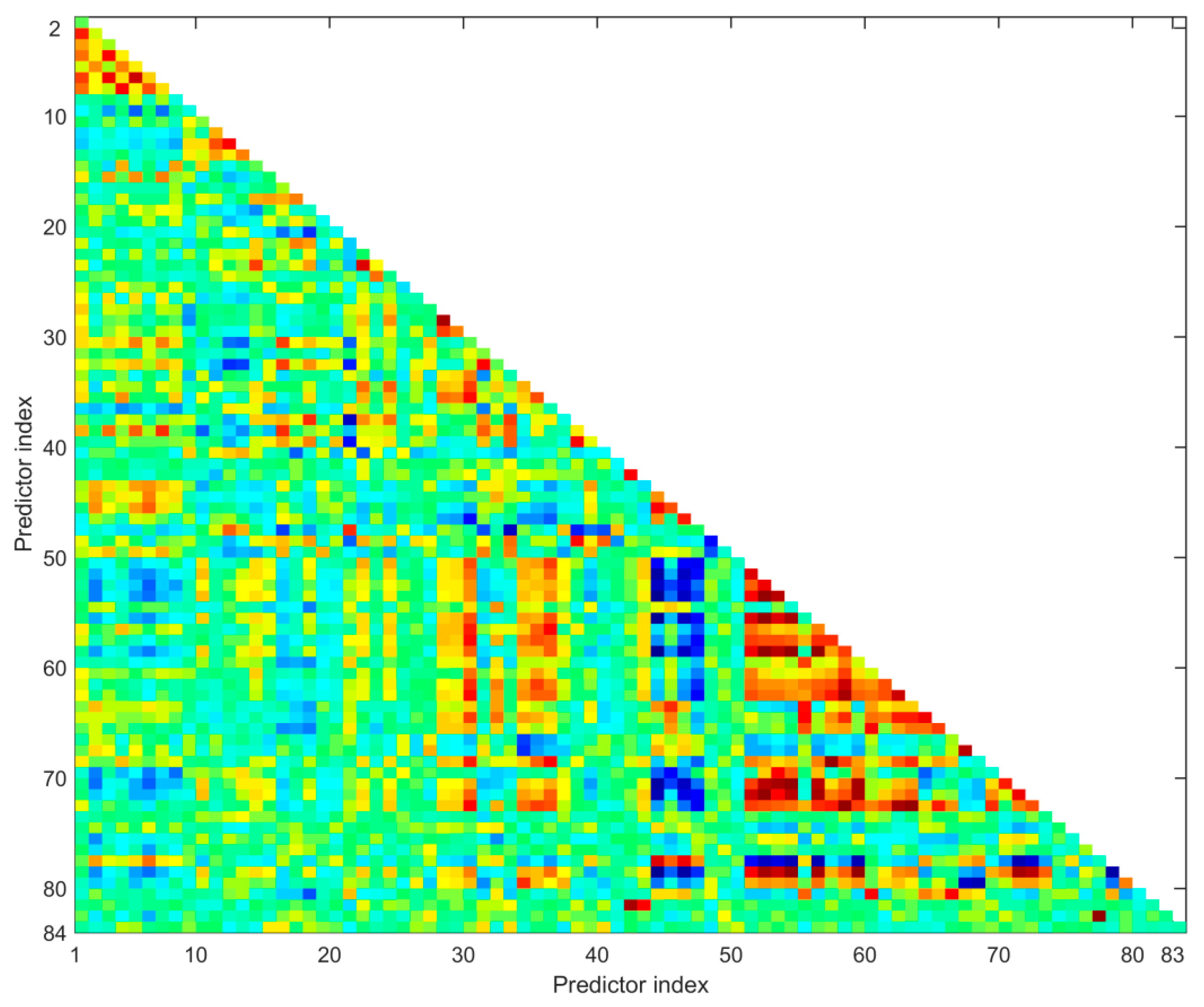
The selection of predictors is an essential procedure in many machine learning problems, especially for the cases of multiple features and small datasets [33,34,35,36]. One of the reasons for this is collinearity amongst predictors. Collinearity refers to the non-independence of predictor variables (sometimes also called multicollinearity; [37,38]). It may inflate the variance of regression parameters in parameter estimation, and lead to the instability of statistical models in predictions [39]. The collinearity of 84 predictors used in this study is simply estimated by linear correlation between every two predictors. The Pearson correlation maps for 84 predictors are shown in Figure 2. It can be seen that many predictors are linearly correlated. The frequency of the Pearson correlation coefficient (CC) amounts to 34 for CCs larger than 0.9 and 19 for CCs larger than 0.95, indicating considerable collinearity amongst predictors. A basic process to eliminate highly correlated predictors is used in the study. The procedures are described as follows:

• Calculate the Pearson CC matrix of all predictors;
• Find the minimum absolute CC between predictor ${\mathrm{x}}_{\mathrm{i}}$ and ${\mathrm{x}}_{\mathrm{j}}$ in the matrix. Terminate the process if the minimum absolute CC is less than the threshold C_thrd;
• Calculate the average absolute CC between ${\mathrm{x}}_{\mathrm{i}}$ and all other predictors, and do the same with ${\mathrm{x}}_{\mathrm{j}}$;
• Remove the predictor with a larger average CC;
• Repeat 2-4.

Above is the first step of the objective predictor selection, which aims to diminish the collinearity of predictors. The threshold C_thrd is chosen dynamically to estimate the influence of collinearity on the prediction model with varying degrees. For C_thrd of 0.3, 0.4, 0.5, 0.6, 0.7, 0.8, and 0.9, 15, 26, 31, 41, 50, 60, and 71 predictors are retained after elimination, respectively. This procedure does not lose much predictive information, since eliminated predictors can be well-represented by at least one of the remaining predictors. Specifically, the maximum values of CCs between each removed predictor and the remaining predictors are shown to be mostly larger than 0.9 (

Table 2. The maximum of correlation coefficients (CCs) between eliminated predictors and remaining predictors. The names of predictors corresponding to the indices are listed in the Appendix A.

Predictor index	28	41	51	53	55	56	57
	58	67	70	72	76	78
CCs	0.99	0.89	0.97	0.97	0.99	0.97	0.81
	0.96	0.95	0.95	0.94	0.93	0.93

).

The second step of the objective predictor selection is to eliminate useless predictors. These predictors provide little predictive information and may raise an overfitting problem of the model. In this study, we employ three different schemes of predictor selection for a comparative analysis, in order to avoid the occasionally good performance of any single scheme and identify a better choice of predictor-selection schemes. The first scheme (single-MLR) is based on the accuracy of the MLR model built with single predictors. The second scheme (F-ratio) is based on an analysis of variance of the predictors [40]. For a single predictor, the F-ratio characterizes the differences in the predictor values among the three PPs. The larger the F-ratio is, the greater the differences in predictor values are. This implies a higher skill of classifying the three PPs for a predictor with a larger F-ratio. The third scheme (L1) is based on the MLR model with L1 regularization introduced in Section 2.2. For predictors selected after step one, they are further selected through the three schemes. The number of predictors (N_pre) is chosen dynamically to search for the optimum parameters.

4. Results

4.1. Training and Validation of the Objective Prediction Model

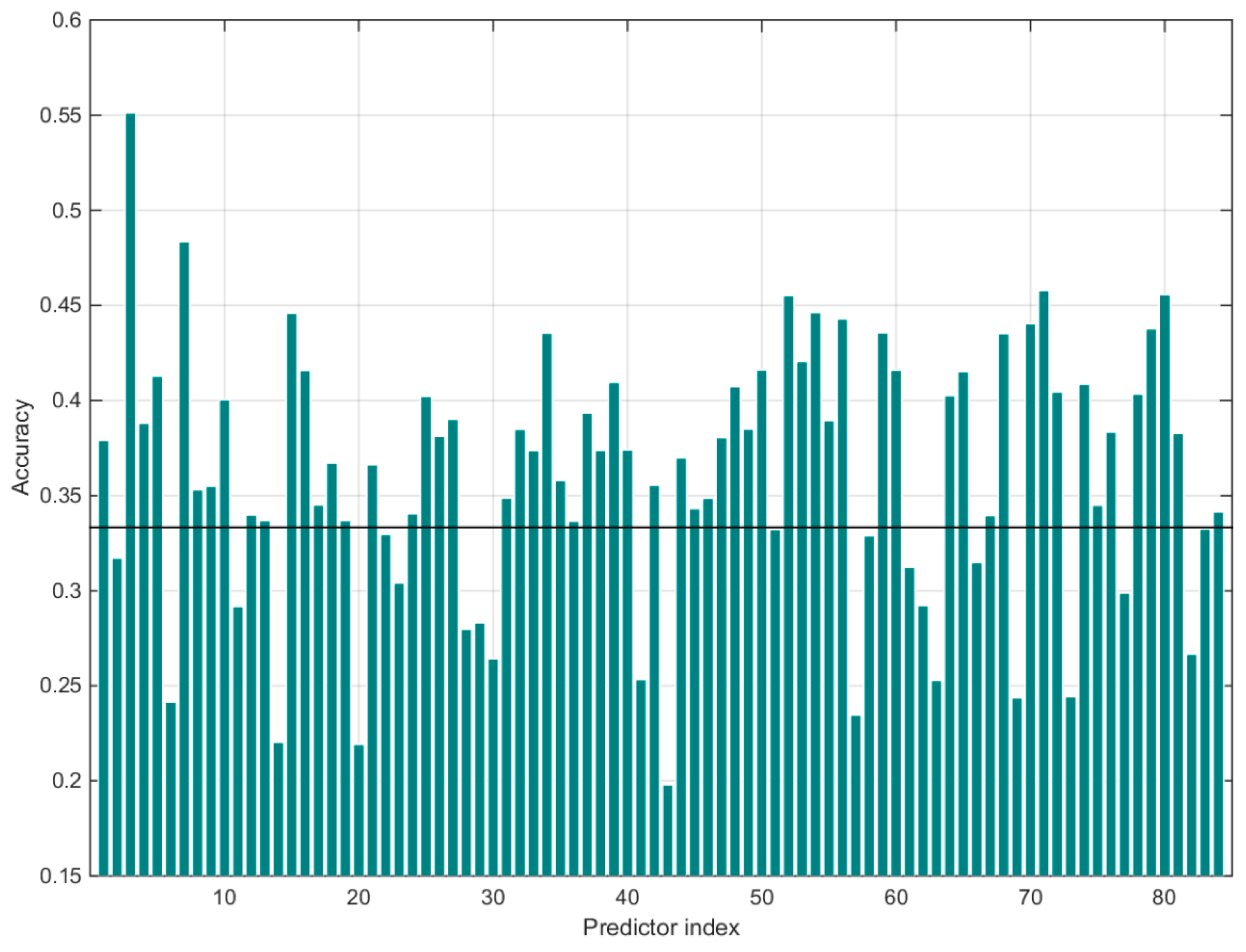
The datasets consist of 61 samples with 21 samples of the largest class. Samples are split into 10 subsets for the stratified 10-fold cross-validation (CV). The stratification here means keeping a relatively constant ratio of the three-class samples in each fold. A robust CV score, which is defined as the mean accuracy of the classification, is obtained by a 1000-times split of the samples. The baseline of the classification accuracy is naturally 1/3. Each predictor is centered and normalized before the procedures of predictor selection. The CV score of the MLR model constructed with every single predictor is tested (Figure 3) to give an overview of the effectiveness of all single predictors. Most of them are found around the baseline, with a mean value of 0.36. The third predictor, the North African–North Atlantic–North American Subtropical High Ridge Position Index, is capable of classifying the three PPs with the highest mean accuracy (0.55). It is hard to answer whether the higher scores are related to certain distinct physical mechanisms between the predictor and the PPs or not. An interpretation from the viewpoint of machine learning is that the summer PP is more likely to be a certain class if a preceding winter climate factor is under certain conditions than it is if other factors are. The situation is similar for multiple combinations of predictors. In the following study, we mainly focus on how well these climate factors tend to make correct classifications.

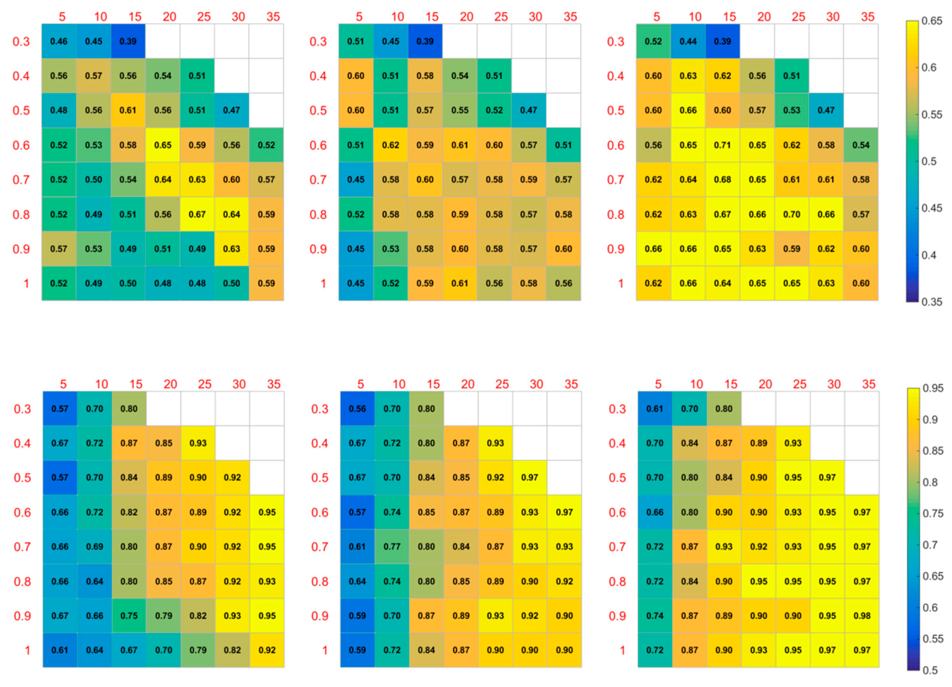
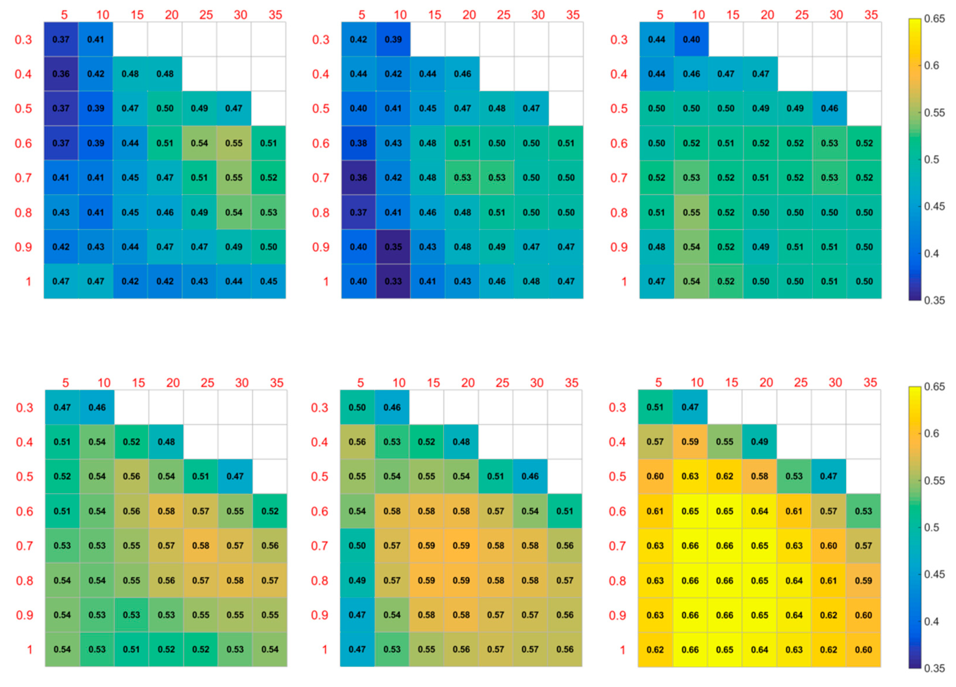
A dynamic experiment is implemented to validate the accuracy with different C_thrds, N_pres, and predictor-selection schemes. C_thrds are chosen from 0.3 to 1, with a stride of 0.1. A C_thrd of 1 means that no predictors are eliminated. N_pres are chosen from 5 to 35, with a stride of 5. The results are shown in the upper panel of Figure 4. Each color block indicates the CV score for selected predictors with fixed C_thrd and N_pre. Apparently, the scores vary with C_thrd and N_pre for all schemes, exhibiting larger values when C_thrd and N_pre are in certain ranges. The CV scores are generally in the range of 0.5–0.7, with the highest scores of 0.67, 0.62, and 0.71 for three schemes, respectively. The scheme L1 shows a higher CV score compared to the other two. Besides, all three schemes show generally higher CV scores than those from single predictors, indicating the higher effectiveness of MLR models with predictor-selection. The CV score here implies the accuracy of objectively recognizing PPs through preceding winter climate factors for the whole observation period.

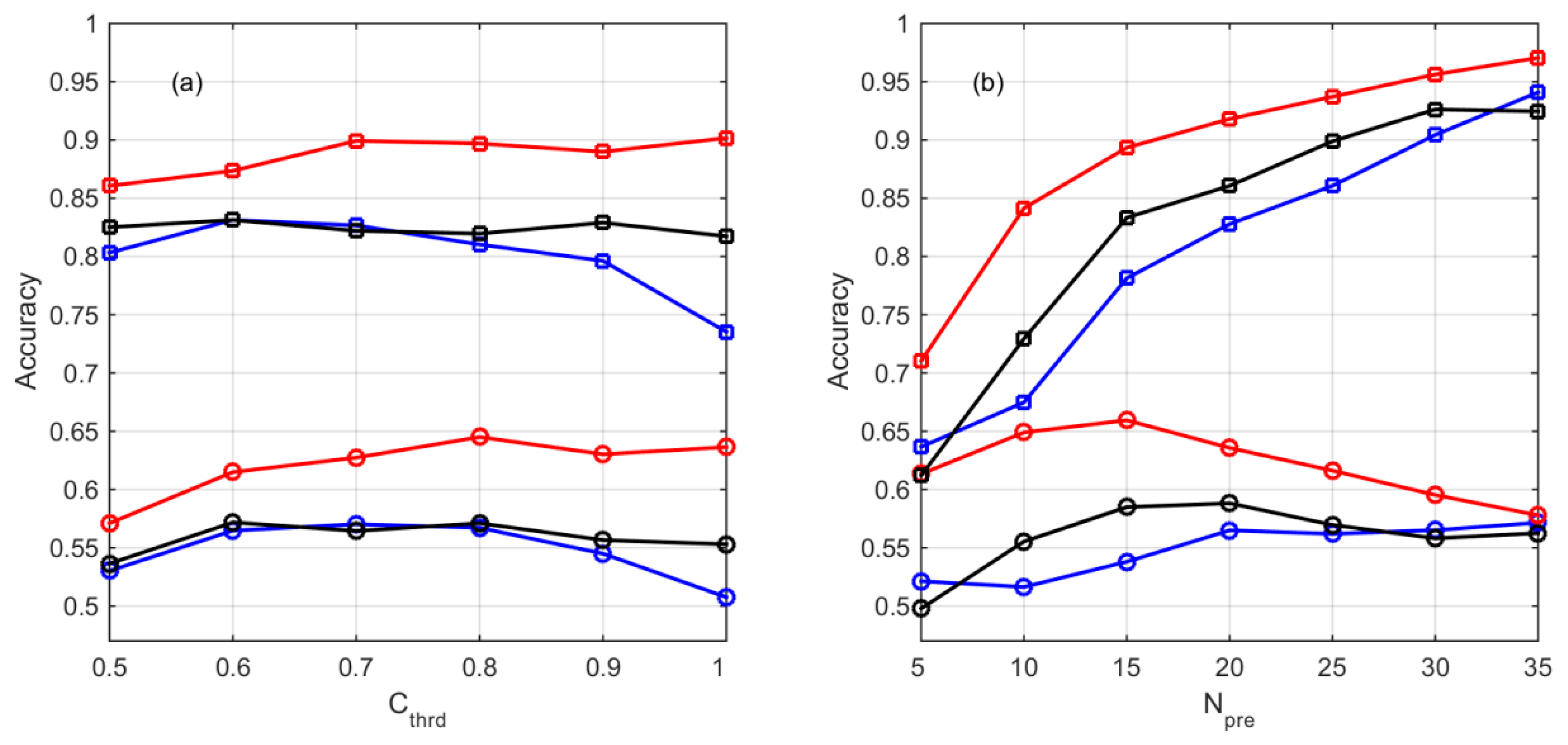
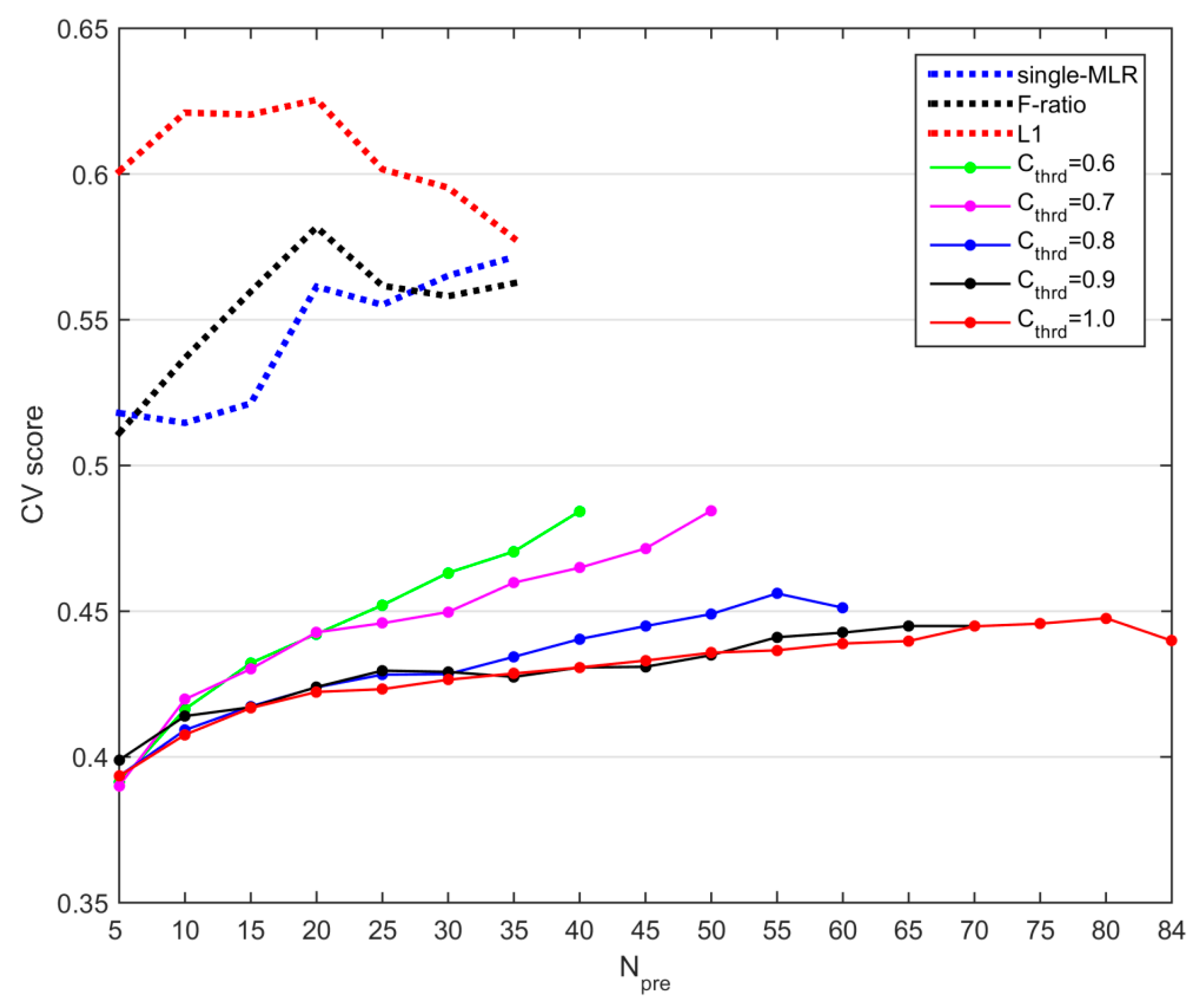
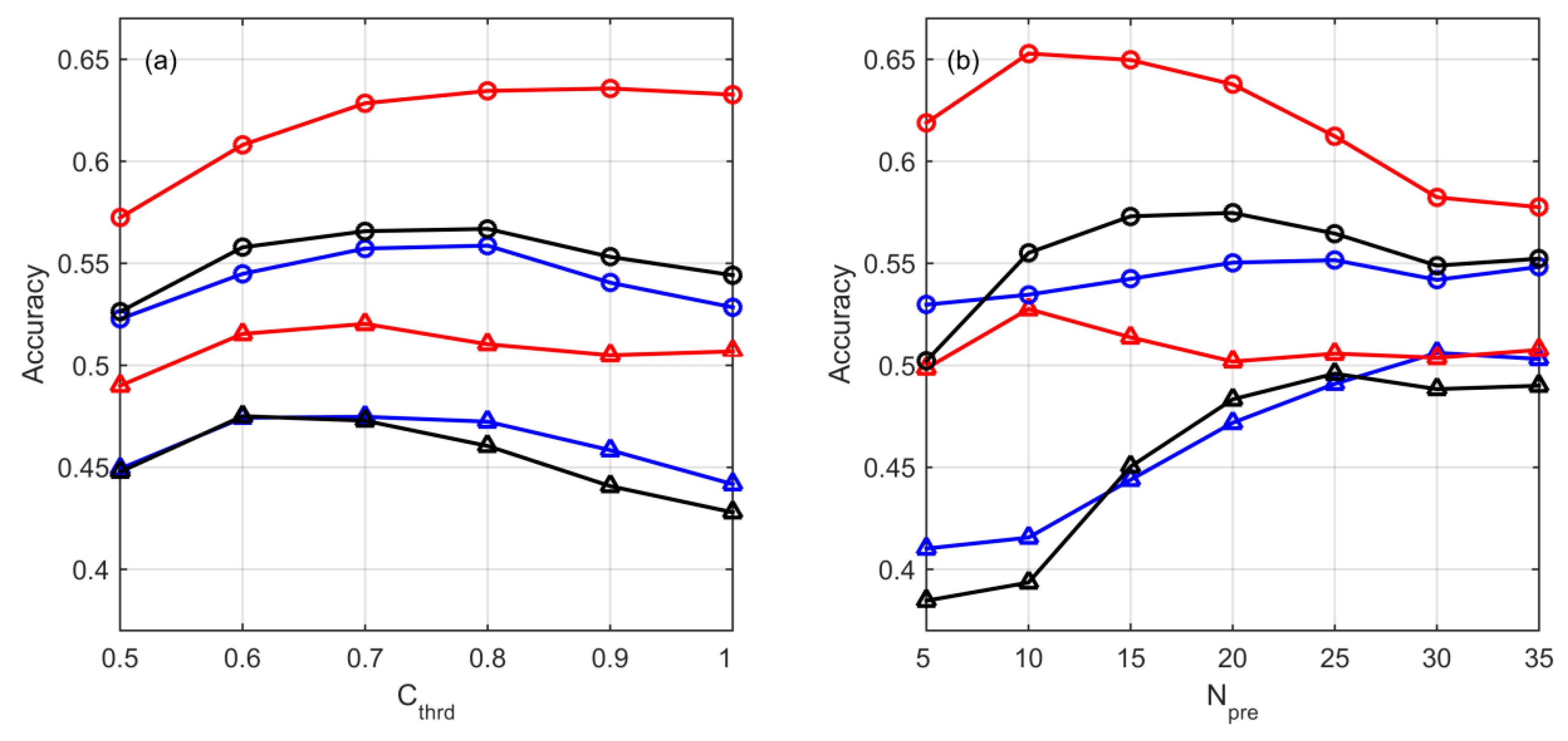
Further relationships between the CV score and different C_thrds and N_pres are investigated. On average, CV scores increase with C_thrds until about 0.8 and then decrease (Figure 5a). This implies the importance of eliminating the collinearity of predictors. The optimum threshold is a compromise between the influence of collinearity and the adequacy of the predictive information. The impact of collinearity is significant for the scheme single-MLR, since the CV score reaches its minimum when no elimination is performed (i.e., C_yhrd = 1). Different behaviors on the influence of collinearity for three schemes probably arise from different processes of predictor selection in step 2. Scheme L1 tends to eliminate correlated predictors internally, and therefore diminishes the influence of collinearity in the prediction model. The predictors selected by the high score of a single predictor based on the scheme single-MLR are correlated to some extent, inducing a lower effectiveness of the prediction model.

Similar features can be found for the relationship between CV score and N_pre (Figure 5b). The CV scores reach their maximum when N_pre equals 15 and 20 for the schemes F-ratio and L1, respectively. For the scheme single-MLR, the CV score increases slightly after reaching a high level at N_pre of 20. In addition, the CV score of the scheme L1 is significantly larger than the other two for small N_pre, implying that scheme L1 is able to select more informative predictors. All these results suggest the importance of the objective selection of predictors in the prediction. The optimal prediction model can only be obtained when collinearity is properly eliminated and the numbers of predictors are properly selected.

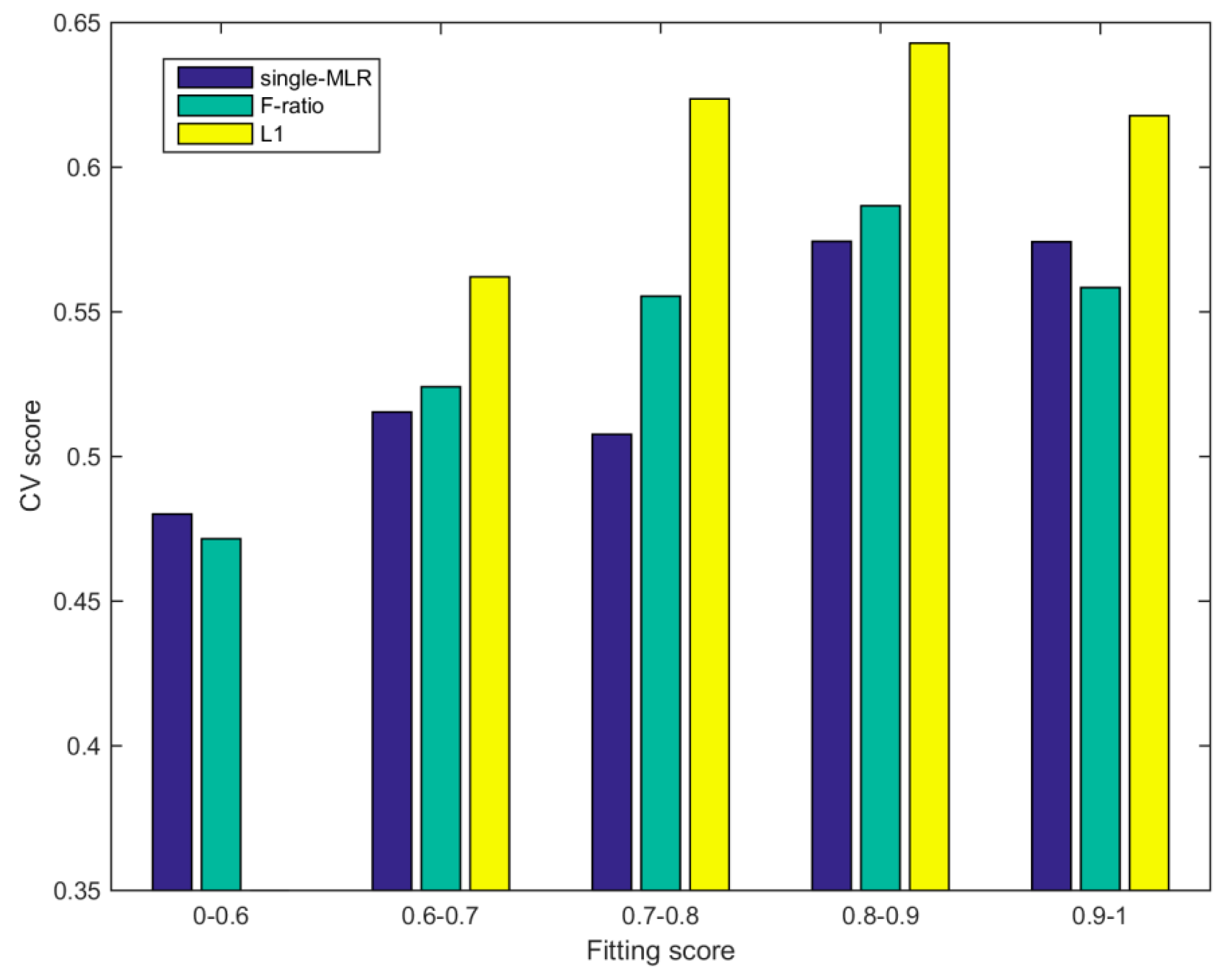
Fitting scores of the MLR model, which indicate the accuracy of training samples, are generally over 0.65, as shown in Figure 4 (lower panel) and Figure 5. The most apparent feature is that the fitting score is higher for a larger number of predictors. It is clearly shown in Figure 5b that the fitting score increases with N_pre and roughly reaches its maximum for the max N_pre. The C_thrd does not have as much of an influence as N_pre on the fitting score, except for the scheme single-MLR, for which the fitting score decreases distinctly when ${\mathrm{C}}_{\mathrm{thrd}}=1$. Histograms of the fitting score for the dynamic experiments are shown in Figure 6. On average, the CV score is not always increasing with the fitting score monotonously. The max CV score appears when the range of the fitting score is 0.8–0.9. Beyond this range, the overfitting problem is serious and the CV score decreases. Further investigation indicates that the overfitting problem mainly originates from the number of predictions. As shown in Figure 5b, the CV score does not increase after N_pre of a range between 15 and 20, while the fitting score keeps increasing.

The experiments indicate that the C_thrds of about 0.6-0.9 and N_pres of 15-20 will generally be the optimal parameters for the objective prediction models. Based on this, a particular model (Model-opt) with C_thrd of 0.8 and N_pre of 15 is chosen to investigate the details of different predictor-selection schemes.

Table 3. Selected predictors sorted in descending order of the importance of the predictors via three predictor-selection schemes with C_thrd of 0.8 and N_pre of 15. Common predictors for three schemes are shaded in green, and gray indicates unique predictors in three schemes. The names of predictors corresponding to the indices are listed in the Appendix A.

Predictors Selection Scheme	Predictor Index
Scheme single-MLR	3 15 70 34 74 53 16 50 48 60 39 64 37 27 25
Scheme F-ratio	3 39 15 16 10 76 27 26 1 50 31 18 4 55 48
Scheme L1	3 37 15 76 4 26 25 70 39 1 75 21 50 19 18

shows 15 indices finally selected via three schemes for the Model-opt model, of which 60 predictors are retained after collinearity elimination. The indices are sorted in descending order by the importance of the predictors. Predictor index No. 3 (North African–North Atlantic–North American Subtropical High Ridge Position), 15 (Pacific Polar Vortex Intensity), and 50 (Atlantic-European Circulation E Pattern Index) are presented in all the three schemes, and the former two indices are always among the top three. The results highlight two precursors, the North African–North Atlantic–North American Subtropical High Ridge Position and the Pacific Polar Vortex Intensity, for summer PPs over eastern China. Besides, more common predictors are presented for every two schemes. These common predictors in different schemes would probably be more valuable in performing predictions.

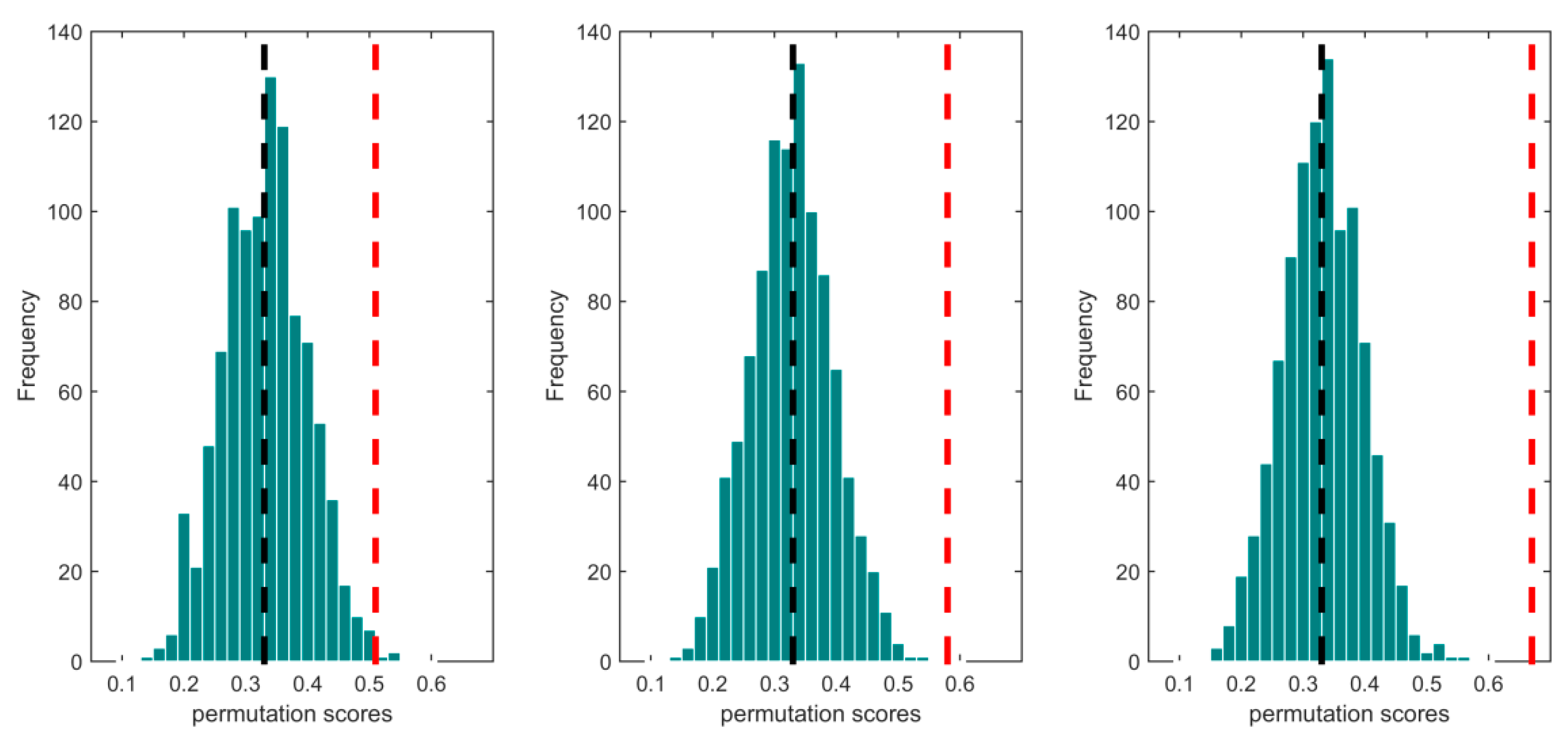
A permutation-based test is applied to evaluate the significance of the classifications. The test assesses whether the model has found a real class structure in the data. The corresponding null distribution is estimated by permuting the labels of the samples [41]. The permutation test is implemented for the Model-opt model described above. First, 61 samples are constructed by randomly permuting the labels of 61 samples, and the permutation scores are then evaluated by the repeated 10-fold CV score. The permutation test is repeated 1000 times to get the null distribution. As shown in Figure 7, the CV scores of the Model-opt model are significantly larger than the permutation scores for all three schemes, implying that the model is able to reveal the intrinsic structure of the predictors corresponding to a certain class.

The effectiveness of the objective prediction model needs to be evaluated. It has already been shown that the average and maximum CV score for individual predictors are generally smaller than those of the objective prediction model. However, it is unknown whether the objective prediction model is superior to the prediction model without predictor selection. The MLR models with different combinations of random-selected predictors are implemented to facilitate a comparative analysis. The repeated 10-fold CV score is used as above. The CV scores of randomly-selected predictors with different numbers are found to be significantly lower than those of objective selection for all schemes (Figure 8). In addition, the CV scores of randomly-selected predictors generally increase with elimination of the collinearity of predictors, but still lower than those of the objective prediction model (Figure 8). This result further confirms the necessity of eliminating the collinearity of predictors and assessing the effectiveness of the objective prediction model. We also notice that the CV score roughly increases with N_pre, which is different from that of the objective prediction model. The reason for this likely arises from the fact that the overfitting problem is more serious when less-informative predictors are added to the objective prediction model. Nonetheless, the MLR model is able to learn much more information from objectively-selected predictors than that from randomly-selected predictors. Moreover, even the MLR model with randomly-selected predictors can also provide useful information for predicting summer PPs, implying the learnable intrinsic relationships between global climate factors and summer PPs over eastern China.

4.2. Generalization Ability of the Objective Prediction Model

The accuracy of the prediction model may decrease in the future due to the non-stationary relationships between summer precipitations and corresponding predictors, as mentioned in the Introduction section. In climatic physics, the main reason for this arises from the fact that the predictors selected based on entire historical records will become less informative for the future period than for the past. The accuracy obtained from the above experiments would consequently be overestimated. This is similar to traditional predictions, which usually overestimate the accuracy of operational prediction. Hence, it is necessary to estimate the influence of non-stationary relationships on predictions, or in other words, estimate the generalization ability of the objective prediction model. Considering there are only a few test samples in observation, an experiment in which predictors are selected based on a random part of the records has since been implemented. All the records are treated as independent samples, and the experiment can be repeated multiple times to get a robust test score. It should be noted that this is different from the CV test in Section 4.1, in which the predictors are selected according to all samples and common predictors are used for all splits in 10-fold tests. The predictor-selection schemes and related parameters C_thrds and N_pres coincide with previous models. To learn as much information as possible from predictors, the training size is maximized and only three samples (one for each class) are used as test sets. Additionally, predictors are centered and normalized for the training sets and then apply the corresponding parameters to the test sets. The experiment is repeated 300 times to obtain stable scores.

The test scores and corresponding CV scores with different C_thrds and N_pres for the three schemes are shown in Figure 9. Similar to Figure 4, the test scores and CV scores also exhibit larger values in certain areas. The test scores are generally in the range of 0.4–0.55, which are smaller than the CV scores of 0.5–0.65. The difference of roughly 0.1 here suggests the influence of non-stationary relationships, as discussed above. Scheme L1 has higher test scores than the other two do, which is coincident with the results of CV scores. However, the maximum test scores of the three schemes are quite close, with values of 0.55, 0.53, and 0.55, respectively. This implies an upper limit of the generalization ability of the prediction model. The standard deviation of CV scores and test scores is ~0.04 and ~0.27, respectively, despite the different C_thrds, N_pres, and schemes.

More details on test scores and corresponding CV scores varying with C_thrds and N_pres are shown in Figure 10. The variations of test scores with C_thrds are coincident with those of CV scores for all three schemes. These highlight the importance of properly eliminating collinearity for prediction. The variations of test scores with N_pres are complicated. For the schemes single-MLR and F-ratio, the test score increases with N_pre until reaching a high level of about 0.5 for N_pre larger than 20. In contrast, for scheme L1, the test scores are maintained at a high level for all N_pres, but with the highest test score at N_pre of 10. The results imply that a high test-score, or in other words, a robust prediction, can be generally obtained by learning information from plenty of predictors. Moreover, high test scores can also be obtained from fewer predictors through a proper method of selection (i.e., scheme L1).

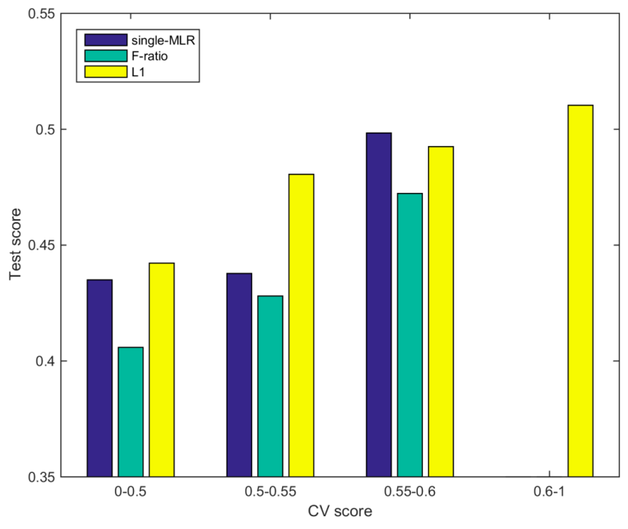
Relationships between test scores and corresponding CV scores are important for assessing the stability of the prediction model. As shown in Figure 11, the test scores are generally increasing with corresponding CV scores, suggesting the worth of improving the training accuracy (CV score) of prediction models. More specifically, for scheme L1, both the test score and corresponding CV score reach the maximum at N_pre of 10. In comparison, for the schemes single-MLR and scheme F-ratio, there is a slight shift. The test scores reach the maximum at N_pre of 30 and N_pre of 25, respectively, and the corresponding CV scores at N_pre of 25 and N_pre of 20 (Figure 10). The prediction model with scheme L1 performs better than the other two, highlighting its application potential for the prediction of summer PPs.

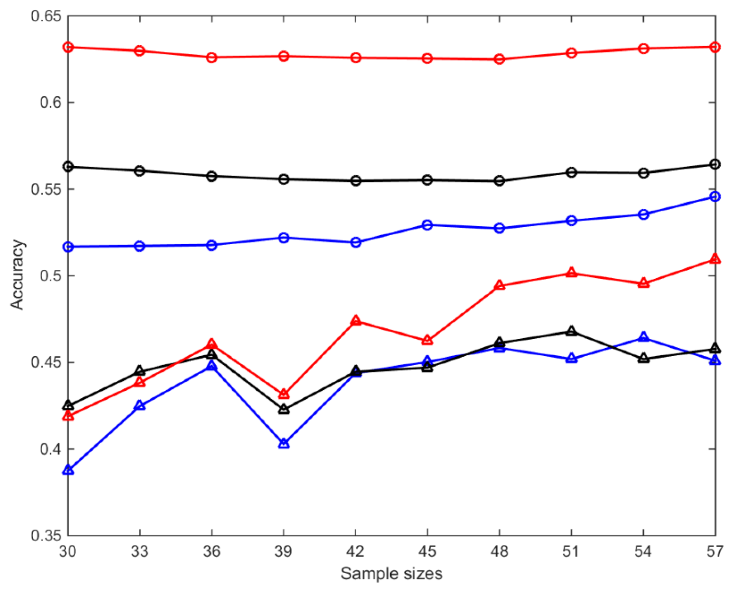
Finally, we try to investigate whether learned information grows with increasing observations. Experiments with different training sizes for three predictor-selection schemes are hence implemented. The N_pres are chosen as 5–35 and the C_thrd is chosen as 0.8. The test size is also set to 3, and the test is repeated 300 times, as described previously. Figure 12 shows the relationships between the average test and CV scores of N_pres and sample size. The test scores are found to generally increase with sample size, while the CV scores are quite smooth. The results confirm that the effectiveness of objective prediction would improve as observation increases. Meanwhile, there probably exists an upper limit of the objective prediction model according to the smooth variations of the CV scores.

5. Summary and Discussion

This article presents a study of the objective prediction of summer PPs over eastern China based on the MLR model. The purpose is to investigate how to learn as much information as possible from various predictors by means of the MLR model, and based on this, to assess the effectiveness of the objective prediction model. The predictors are objectively, not limited by physical mechanisms, selected from 84 preceding winter climate factors. Three predictor-selection schemes are involved in the study. The optimal prediction model together with the influence of collinearity on predictors and numbers of predictors are estimated through varied parameters C_thrd and N_pre.

The CV scores are found to be higher within certain ranges of C_thrd and N_pre for all schemes, suggesting that the optimal prediction model can only be obtained when collinearity is properly eliminated, and the number of predictors is properly selected. C_thrds of about 0.6–0.9 and N_pres of 15–20 are found to be roughly the optimal parameters for the objective predictions. The highest scores are comparable with traditionally-estimated upper limits of predictability with a range of 0.6–0.7 [42], reflecting the effectiveness of the objective prediction method. Moreover, the MLR model is found to be able to reveal the intrinsic structure of the predictors corresponding to a certain class and to learn much more information from objectively selected predictors than that from randomly selected predictors and a single predictor. All the results suggest the importance and effectiveness of objective selections of predictors for predictions.

The generalization ability of the objective prediction model is assessed by experiments of which predictors are selected based on a part of the records. The test scores decrease by roughly 0.1 on average compared to corresponding CV scores, suggesting the influence of non-stationary relationships between summer precipitation patterns and corresponding predictors on predictions. The results suggest that a robust prediction can be generally obtained by learning information from plenty of predictors, although the highest test score may be obtained from fewer predictors through a proper method of predictor selection. This study also implies that an upper limit of the objective prediction model probably exists, and the limit is coincident with the predictability analyzed by other studies [42]. Besides, the results suggest that the effectiveness of objective prediction would generally improve as observation increases, highlighting its potential usage in the operational prediction of summer PPs.

Two nonlinear machine learning methods (random forest and multi-layer perceptron) are used to test the influence of different methods on the results with respect to objective selections of predictors (results not shown). The CV scores obtained by these two nonlinear methods are comparable to the MLR model, although the fitting scores are very high. The major problem in the prediction of summer PPs over eastern China is the shortage of observations and the influence of the non-stationarity of the climate system. Consequently, it is hard to find effective predictors, specifically, robust relationships between individual preceding winter climate factors and summer PPs. Even for predictors with reasonable physical mechanisms, the relationships would change along with climate change, let alone physical mechanisms related to other predictors, which may be dominant during the other periods. The circumstance would be worse if few predictors were selected [27]. Multiple predictors objectively selected from the global climate may partly overcome this problem, and this is the most important motive for performing this study.

It is notable that the summer PPs were treated as independent samples in this study, which would overestimate the predictability to some extent. We also tested the model Model-opt with scheme L1 with training samples of the years 1952–1992, 1952–1993 … 1952–2011 and testing samples of 1993, 1994 … 2012. The test score is also about 0.5, suggesting that this assumption is reasonable. On the other hand, additional signals may be found from previous summer PPs since they are essentially time-dependent. How to involve the time-dependent information in the objective prediction model is worth considering in further studies. Nevertheless, this objective approach provides a meaningful baseline for the prediction of summer PPs in eastern China. This study expands and improves the knowledge of prediction of summer PPs over eastern China, and the objective approach can also be applied for the prediction of other regional climate events.

References

1. Song, J. Changes in dryness/wetness in China during the last 529 years. Int. J. Climatol. 2000, 20, 1003–1015. [Google Scholar] [CrossRef]
2. Wei, F.Y. An integrative estimation model of summer rainfall-band patterns in China. Prog. Nat. Sci. Mater. 2007, 17, 280–288. [Google Scholar]
3. Huang, J.P.; Yi, Y.H.; Wang, S.W.; Chou, J.F. An analogue-dynamical long-range numerical weather prediction system incorporating historical evolution. Q. J. R. Meteorol. Soc. 1993, 119, 547–565. [Google Scholar] [CrossRef]
4. Wang, B.; Ding, Q.H.; Fu, X.H.; Kang, I.S.; Jin, K.; Shukla, J.; Doblas-Reyes, F. Fundamental challenge in simulation and prediction of summer monsoon rainfall. Geophys. Res. Lett. 2005, 32. [Google Scholar] [CrossRef] [Green Version]
5. Wang, H.J.; Fan, K.; Sun, J.Q.; Li, S.L.; Lin, Z.H.; Zhou, G.Q.; Chen, L.J.; Lang, X.M.; Li, F.; Zhu, Y.L.; et al. A Review of Seasonal Climate Prediction Research in China. Adv. Atmos. Sci. 2015, 32, 149–168. [Google Scholar] [CrossRef]
6. Yang, Y.M.; Wang, B.; Li, J. Improving Seasonal Prediction of East Asian Summer Rainfall Using NESM3.0: Preliminary Results. Atmosphere 2018, 9, 487. [Google Scholar] [CrossRef]
7. Liu, Y.; Fan, K. Improve the prediction of summer precipitation in the Southeastern China by a hybrid statistical downscaling model. Meteorol. Atmos. Phys. 2012, 117, 121–134. [Google Scholar] [CrossRef]
8. Wang, H.J.; Fan, K. A New Scheme for Improving the Seasonal Prediction of Summer Precipitation Anomalies. Weather. Forecast. 2009, 24, 548–554. [Google Scholar] [CrossRef]
9. Ding, Y.H.; Chan, J.C.L. The East Asian summer monsoon: An overview. Meteorol. Atmos. Phys. 2005, 89, 117–142. [Google Scholar] [CrossRef]
10. Zhou, T.J.; Yu, R.C. Atmospheric water vapor transport associated with typical anomalous summer rainfall patterns in China. J. Geophys. Res. Atmos. 2005, 110. [Google Scholar] [CrossRef] [Green Version]
11. Wang, B.; Xiang, B.Q.; Lee, J.Y. Subtropical High predictability establishes a promising way for monsoon and tropical storm predictions. Proc. Natl. Acad. Sci. USA 2013, 110, 2718–2722. [Google Scholar] [CrossRef] [PubMed] [Green Version]
12. Wang, H.J.; Xue, F.; Zhou, G.Q. The spring monsoon in South China and its relationship to large-scale circulation features. Adv. Atmos. Sci. 2002, 19, 651–664. [Google Scholar]
13. Liu, X.F.; Yuan, H.Z.; Guan, Z.Y. Effects of Enso on the Relationship between Iod and Summer Rainfall in China. J. Trop. Meteorol. 2009, 15, 59–62. [Google Scholar] [CrossRef]
14. Storch, H.V.; Zorita, E.; Cubasch, U. Downscaling of Global Climate Change Estimates to Regional Scales: An Application to Iberian Rainfall in Wintertime. J. Clim. 1993, 6, 1161–1171. [Google Scholar] [CrossRef] [Green Version]
15. Wu, Z.W.; Wang, B.; Li, J.P.; Jin, F.F. An empirical seasonal prediction model of the east Asian summer monsoon using ENSO and NAO. J. Geophys. Res. Atmos. 2009, 114. [Google Scholar] [CrossRef] [Green Version]
16. Cao, Q.; Hao, Z.C.; Yuan, F.F.; Su, Z.K.; Berndtsson, R. ENSO Influence on Rainy Season Precipitation over the Yangtze River Basin. Water 2017, 9, 469. [Google Scholar] [CrossRef]
17. Huang, R.H.; Wu, Y.F. The influence of ENSO on the summer climate change in China and its mechanism. Adv. Atmos. Sci. 1989, 6, 21–32. [Google Scholar] [CrossRef]
18. Wu, Z.W.; Li, J.P.; Jiang, Z.H.; He, J.H.; Zhu, X.Y. Possible effects of the North Atlantic Oscillation on the strengthening relationship between the East Asian Summer monsoon and ENSO. Int. J. Climatol. 2012, 32, 794–800. [Google Scholar] [CrossRef]
19. Zhao, P.; Zhou, Z.J.; Liu, J.P. Variability of Tibetan spring snow and its associations with the hemispheric extratropical circulation and East Asian summer monsoon rainfall: An observational investigation. J. Clim. 2007, 20, 3942–3955. [Google Scholar] [CrossRef]
20. Wu, Z.W.; Li, J.P.; Jiang, Z.H.; Ma, T.T. Modulation of the Tibetan Plateau Snow Cover on the ENSO Teleconnections: From the East Asian Summer Monsoon Perspective. J. Clim. 2012, 25, 2481–2489. [Google Scholar] [CrossRef]
21. Sung, M.K.; Kwon, W.T.; Baek, H.J.; Boo, K.O.; Lim, G.H.; Kug, J.S. A possible impact of the North Atlantic Oscillation on the east Asian summer monsoon precipitation. Geophys. Res. Lett. 2006, 33. [Google Scholar] [CrossRef]
22. Gu, W.; Li, C.; Li, W.; Zhou, W.; Chan, J.C.L. Interdecadal unstationary relationship between NAO and east China’s summer precipitation patterns. Geophys. Res. Lett. 2009, 36. [Google Scholar] [CrossRef]
23. Liao, Q.S.; Zhao, Z.G. A seasonal forecasting scheme on precipitation distribution in summer in China. Quart. J. Appl. Meteor. 1992, 3 (Suppl. 1), 1–9. (In Chinese) [Google Scholar]
24. Fan, K.; Lin, M.; Gao, Y. Forecasting the summer rainfall in North China using the year-to-year increment approach. Sci. China Earth Sci. 2009, 52, 532–539. [Google Scholar] [CrossRef]
25. Yim, S.-Y.; Wang, B.; Xing, W.J. Prediction of early summer rainfall over South China by a physical-empirical model. Clim. Dyn. 2014, 43, 1883–1891. [Google Scholar] [CrossRef]
26. Chen, X.F.; Zhao, Z.G. The Application and Research on Predication of China Rainy Season Rainfall; Meteorological Press: Beijing, China, 2000. (In Chinese) [Google Scholar]
27. Zhao, J.H.; Feng, G.L. Reconstruction of conceptual prediction model for the Three Rainfall Patterns in the summer of eastern China under global warming. Sci. China Earth Sci. 2014, 57, 3047–3061. [Google Scholar] [CrossRef]
28. Liao, Q.S.; Chen, G.Y.; Chen, G.Z. Collection of Long Time Weather Forecast; China Meteorological Press: Beijing, China, 1981; pp. 103–114. (In Chinese) [Google Scholar]
29. Wei, F.Y.; Zhang, X.G. The classification and forecasting of summer rain-belt in the east part of China. Meteorol. Mon. 1988, 14, 15–19. (In Chinese) [Google Scholar]
30. Bishop, C.M. Pattern Recognition and Machine Learning; Springer: New York, NY, USA, 2006. [Google Scholar]
31. Yan, H.S.; Yang, S.Y.; Hu, J.; Chen, J.G. A Study of the relationship between the winter middle-high latitude atmospheric circulation change and the principal rain patterns in rainy season over China. Chin. J. Atmos. Sci. 2006, 30, 285–292. (In Chinese) [Google Scholar]
32. Sanderson, M.G.; Economou, T.; Salmon, K.H.; Jones, S.E.O. Historical Trends and Variability in Heat Waves in the United Kingdom. Atmosphere 2017, 8, 191. [Google Scholar] [CrossRef]
33. Pour, S.H.; Bin Harun, S.; Shahid, S. Genetic Programming for the Downscaling of Extreme Rainfall Events on the East Coast of Peninsular Malaysia. Atmosphere 2014, 5, 914–936. [Google Scholar] [CrossRef] [Green Version]
34. Seo, J.H.; Lee, Y.H.; Kim, Y.H. Feature Selection for Very Short-Term Heavy Rainfall Prediction Using Evolutionary Computation. Adv. Meteorol. 2014, 203545. [Google Scholar] [CrossRef]
35. Wei, C.C.; Peng, P.C.; Tsai, C.H.; Huang, C.L. Regional Forecasting of Wind Speeds during Typhoon Landfall in Taiwan: A Case Study of Westward-Moving Typhoons. Atmosphere 2018, 9, 141. [Google Scholar] [CrossRef]
36. Lyu, B.L.; Zhang, Y.H.; Hu, Y.T. Improving PM2.5 Air Quality Model Forecasts in China Using a Bias-Correction Framework. Atmosphere 2017, 8, 147. [Google Scholar] [CrossRef]
37. Alin, A. Multicollinearity. WIREs Comp. Stat. 2010, 2, 370–374. [Google Scholar] [CrossRef]
38. Jin, L.; Huang, X.Y.; Shi, X.M. A Study on Influence of Predictor Multicollinearity on Performance of the Stepwise Regression Prediction Equation. Acta Meteorol. Sin. 2010, 24, 593–601. [Google Scholar]
39. Dormann, C.F.; Elith, J.; Bacher, S.; Buchmann, C.; Carl, G.; Carre, G.; Marquez, J.R.G.; Gruber, B.; Lafourcade, B.; Leitao, P.J.; et al. Collinearity: A review of methods to deal with it and a simulation study evaluating their performance. Ecography 2013, 36, 27–46. [Google Scholar] [CrossRef]
40. Hogg, R.V.; Craig, A.T. Introduction to Mathematical Statistics, 5th ed.; Prentice Hall: Upper Saddle River, NJ, USA, 1995. [Google Scholar]
41. Ojala, M.; Garriga, G.C. Permutation Tests for Studying Classifier Performance. J. Mach. Learn. Res. 2010, 11, 1833–1863. [Google Scholar]
42. Wang, S.W. Advances in Modern Climatology; China Meteorological Press: Beijing, China, 2002. (In Chinese) [Google Scholar]
Figure 1. Typical precipitation patterns of class I (left), II (middle), and III (right) over eastern China. The contoured data is the average of the percentage of anomalies of summer precipitation during 1961–2012 for each class according to Table 2, respectively. The thick black line to the north of 32° N indicates the Yellow River and that to the south indicates the Yangtze River. The original precipitation data is available from a gridded dataset for China (http://data.cma.cn/data/detail/dataCode/SURF_CLI_CHN_PRE_MON_GRID_0.5).
Atmosphere 10 00213 g001
Figure 2. Pearson correlation maps for 84 predictors selected in the study during 1952–2012. The names of predictors corresponding to the indices are listed in the Appendix A.
Atmosphere 10 00213 g002
Figure 3. The repeated 10-fold cross-validation (CV) score of the multinomial logistic regression (MLR) model using one individual predictor. The black line indicates the baseline of the classification accuracy of 0.33. The names of predictors corresponding to the indices are listed in the Appendix A.
Atmosphere 10 00213 g003
Figure 4. The repeated 10-fold CV scores (upper panel) and fitting scores (lower panel) for different Cthrds and Npres, and predictor-selection schemes single-MLR (left panel), F-ratio (middle panel), and L1 (right panel).
Atmosphere 10 00213 g004
Figure 5. (a) The average repeated 10-fold CV scores (circle) and fitting scores (square) of all Npres dependent on Cthrds, for the schemes single-MLR (blue), F-ratio (black), and L1 (red), respectively. (b) The same as (a), but for the average scores of Cthrds in the range of 0.5-1 dependent on Npres.
Atmosphere 10 00213 g005
Figure 6. Histogram of the fitting scores with respect to CV scores (data refer to Figure 4) for three schemes, respectively.
Atmosphere 10 00213 g006
Figure 7. Histograms of permutation scores evaluated from the objective prediction model with Cthrd of 0.8 and Npre of 15 by 1000 times for the schemes single-MLR (left panel), F-ratio (middle panel), and L1 (right panel), respectively. The red dashed line indicates the CV score of the Model-opt model.
Atmosphere 10 00213 g007
Figure 8. The repeated 10-fold CV scores (valid line) for MLR models with randomly-selected predictors dependent on different Npres and Cthrds. The CV scores of the objective prediction model (dashed line; refers to Figure 5) are shown for comparison.
Atmosphere 10 00213 g008
Figure 9. The test scores (upper panel) and repeated 10-fold CV scores (lower panel) for different Cthrds and Npres, and predictor-selection schemes single-MLR (left panel), F-ratio (middle panel), and L1 (right panel).
Atmosphere 10 00213 g009
Figure 10. (a) The test scores (circle) and average repeated 10-fold CV scores (square) of all Npres dependent on Cthrds, for the schemes single-MLR (blue), F-ratio (black), and L1 (red). (b) The same as (a), but for the average scores of Cthrds in the range of 0.5–1 dependent on Npres.
Atmosphere 10 00213 g010
Figure 11. Histogram of the CV scores with respect to test scores in Figure 9 for three schemes, respectively.
Atmosphere 10 00213 g011
Figure 12. The average test scores (triangle) and repeated 10-fold CV scores (circle) for Npres of 5–35 and Cthrd of 0.8 dependent on sample sizes for the schemes single-MLR (blue), F-ratio (black), and L1 (red).
Atmosphere 10 00213 g012