Article

Future Changes of Precipitation over the Han River Basin Using NEX-GDDP Dataset and the SVR_QM Method

1
School of Resource and Environmental Science, Wuhan University, 129 Luoyu Road, Wuhan 430079, China
2
State Key Laboratory of Information Engineering in Surveying, Mapping, and Remote Sensing, Wuhan University, 129 Luoyu Road, Wuhan 430079, China
3
Collaborative Innovation Center of Geospatial Technology, Wuhan University, Wuhan 430079, China
*
Author to whom correspondence should be addressed.
Atmosphere 2019, 10(11), 688; https://doi.org/10.3390/atmos10110688
Submission received: 17 October 2019 / Revised: 3 November 2019 / Accepted: 5 November 2019 / Published: 8 November 2019
(This article belongs to the Section Meteorology)

Abstract

:
After the release of the high-resolution downscaled National Aeronautics and Space Administration (NASA) Earth Exchange Global Daily Downscaled Projections (NEX-GDDP) dataset, it is worth exploiting this dataset to improve the simulation and projection of local precipitation. This study developed support vector regression (SVR) and quantile mapping (SVR_QM) ensemble and correction models on the basis of historic precipitation in the Han River basin and the 21 NEX-GDDP models. The generated SVR_QM models were applied to project changes of precipitation during the 21st century for the region. Several statistical metrics, including Pearson’s correlation coefficient (PCC), root mean squared error (RMSE), and relative bias (Rbias), were used for evaluation and comparative analyses. The results demonstrated the superior performance of SVR_QM compared with multi-layer perceptron (MLP), SVR, and random forest (RF), as well as simple model average (MME) ensemble methods and single NEX-GDDP models. PCC was up to 0.84 from 0.61–0.71 for the single NEX-GDDP models, RMSE was up to 34.02 mm from 48–51 mm, and Rbias values were almost removed. Additionally, the projected precipitation changes during the 21st century in most stations had an increasing trend under both Representative Concentration Pathway RCP4.5 and RCP8.5 emissions scenarios; the regional average precipitation during the middle (2040–2059) and late (2070–2089) 21st century increased by 3.54% and 5.12% under RCP4.5 and by 7.44% and 9.52% under RCP8.5, respectively.

1. Introduction

Extreme weather will occur more frequently under the background of global warming. As a result, human society, economy, life, and natural ecosystems will be more affected [1,2]. It is essential for researchers, managers, and citizens to know the future climate change trends so that losses caused by extreme disasters can be minimized as much as possible by effective preventive measures.
General circulation models (GCMs) are one of the most important and feasible methods for predicting future large-scale climate change and have become a major research tool in the field of global change [3,4,5]. However, it is difficult for GCMs to understand and adequately model climate systems due to their complexity and topography, and large uncertainties thus exist in their projections, especially at the regional scale. As a method of transforming the output information of large-scale and low-resolution global climate models into regional climate change information at small scales and high resolution, downscaling technology can obtain more refined precipitation variation characteristics, reduce the simulation error of regional precipitation to a certain extent, and thus improve regional precipitation forecasts. Therefore, downscaling techniques are vital for transformation from large scales to small scales. There are many downscaling applications in existence, including dynamical downscaling and statistical downscaling, which have improved projections of climate factors at finer scales [6,7,8]. Recently, National Aeronautics and Space Administration (NASA) produced Earth Exchange Global Daily Downscaled Projections (NEX-GDDP), which used statistical downscaling to downscale 21 GCMs from the Coupled Model Intercomparison Project 5 (CMIP5) and generate a high-resolution dataset. NEX-GDDP provides global-scale, high-resolution (spatial resolution: 0.25° longitude × 0.25° latitude) data and corrects the deviation of future estimates. It can be referenced to assess the impact of climate change and provide more refined future climatic estimates. It facilitates the study of high-resolution future climate change at the regional scale, especially in the middle and lower reaches of the Yangtze River basin, which has complex topography and climate sensitivity. After its release, the NEX-GDDP dataset was applied to study the near- and long-term climate, and proved to be robust, even in regions with complex topography [9,10], although there are findings that NEX-GDDP is consistent with historical observations only at the monthly scale [11].
There are large uncertainties in the projection of future climate change. Multi-model ensemble methods have been applied and were found to effectively reduce the uncertainties; ensemble simulation outperformed the ‘best’ single model over the short or long term [12]. There are some typical ensemble methods, such as the simple model average (MME), Bayesian model average (BMA), and reliability ensemble average (REA) [13,14], which have a certain ability to alleviate GCM uncertainty. However, the relationship between multi NEX-GDDP and observed precipitation are often very complex. Machine learning (ML) approaches have been thought to be efficient for modelling highly nonlinear relationships [15]. On the basis of their incorporated layers and nodes and excitation mechanism, artificial neural networks (ANNs) have been successfully applied to climate downscaling and have also been able to establish high nonlinear relationships between predictors and observed precipitation [16]. Additionally, the support vector regression (SVR) model has also been able to capture nonlinear relationships with its kernel function mechanism, which maps low-dimensional input data to a high-dimensional feature space [17]. Another ML method, random forest (RF), is also a competent and robust algorithm that can avoid overfitting, be compatible with different types of input variables, and operate flexibly. These ML methods have been widely and successfully used to downscale GCM climatic factors to local levels [18,19]. Sa’adi et al. compared RF and SVR to downscale monthly precipitation on the basis of model output statistics, which established the relationship between multi-grid precipitation and observed station precipitation [20]. These results proved the ability of SVR and RF for such applications. In addition, although the SVR method performed better overall, RF was better for some stations. The structure of the ensemble model in this study was similar to the principle mentioned above; unfortunately, literature exploring the capacity of ML for ensemble NEX-GDDP is lacking. It will be interesting to study and compare the performance of ANN, SVR, and RF for ensemble NEX-GDDP precipitation modelling.
Precipitation bias after ensemble simulation always remains, and the less the bias between ensemble outputs and observations, the more reliable the future projection based on these data [21,22]. Generally, there are two methods to correct the bias: one corrects the predictor variables before downscaling, and the other corrects the bias between downscaled precipitation and observations. The latter approach is appropriate for NEX-GDDP data. There is an effective method, quantile mapping (QM), which has been successfully applied for many precipitation bias-corrected studies [23,24,25] and is considered the most efficient method [26]. This study first attempted to combine the SVR methods for ensemble simulation and the QM method for bias correction on the basis of 21 NEX-GDDP precipitation models in the Han River basin to improve the reliability of future projections under the Representative Concentration Pathway (RCP)4.5 and RCP8.5.
The first purpose of this study was to explore the superiority of support vector regression and quantile mapping (SVR_QM) methods for ensemble simulation and the correction of historic NEX-GDDP precipitation to improve the reliability of projection. The major objectives of the paper were to (1) develop station-based SVR_QM ensemble and correction models for NEX-GDDP precipitation in the Han River basin; (2) study the comparison of the ensemble prediction ability of MLP, SVM, and RF for NEX-GDDP precipitation; and (3) project the changes of monthly precipitation in the 21st century on the basis of SVR_QM models under RCP4.5 and RCP8.5 in the Han River basin. The contribution of the present study was the exploitation of the SVR_QM methods and NEX-GDDP data that was done to improve the reliability of precipitation simulation and projection at the regional scale in the Han River basin. Improved projections of high-resolution precipitation will be more beneficial for the guidance of long-term management strategies such as water resources allocation, flood mitigation, and ecological layout.
The remainder of this paper is formulated as follows: Section 2 introduces the Materials and Methods, including the topographical and climatic conditions of the Han River basin, the observed data used and NEX-GDDP data, and the methodology in this study. Section 3 depicts and discusses the results. Finally, several conclusions and prospects from this study are presented.

2. Materials and Methods

2.1. Study Area and Data

The Han River is the main tributary of the middle reaches of the Yangtze River; it is 1577 km long and covers 159 thousand km2. In the Han River basin, the river system is veined and contains many tributaries. The upper reaches mainly include mountains and hills, whereas the lower reaches include the Jianghan plain. Over the past 50 years, the average annual rainfall has been approximately 700–1100 mm. The Han River basin has been suffering from flood and drought since the 1990s due to the integrated effects of natural and human factors. In this study, 21 meteorological stations in the Han River basin were selected on the basis of the principle of data continuity and integrity. In addition, the observed precipitation of eight stations around the Han River were used only to compute the mean precipitation of the region. The observed daily precipitation data in the Han River were used to train and validate the ensemble and mapping models in the period from 1961 to 2005. These data were acquired from the website of China Meteorological Data [27]. Figure 1 depicts the river system, altitudes and the distribution of 21 stations on the Han River, and 8 stations around the Han River basin. Table 1 describes the position information for these stations. The stations 1–21 represent the stations on the Han River, and the remaining eight stations represent the stations around the Han River basin.
Regarding the NEX-GDDP data, the downscaled historical precipitation and 21st century precipitation data under the RCP4.5 and RCP8.5 scenarios were chosen for this region. NEX-GDDP is a novel high-resolution (0.25° longitude × 0.25° latitude) daily downscaled dataset released in June 2015 by NASA. Specifically, the NEX-GDDP, which is called ‘NASA Earth Exchange Global Daily Downscaled Projections’, was generated from 21 CMIP5 model simulations based on bias-correction spatial disaggregation (BCSD) downscaling technology [28]. Three climatic variables were included in this dataset: daily precipitation and maximum and minimum temperature. The time span included the historical period of 1950–2005 and the future period of 2006–2100 (RCP4.5 and RCP8.5 runs). The total storage space of the dataset source file (*.nc) was more than 12 terabyte (TB). Table 2 describes the RCP4.5 and RCP8.5 scenarios and Table 3 shows the 21 GCM models used that were downscaled to obtain NEX-GDDP.
An official website provides more details on this dataset [29], which can be freely acquired via the https://cds.nccs.nasa.gov/nex-gddp/ website. In this study, the global 21 NEX-GDDP precipitation data were downloaded. In the process of evaluating the simulation ability of NEX-GDDP, the average of the data for the nine grid cells nearest to the observed station was regarded as the simulation precipitation for the corresponding station. On the basis of the global data, the monthly simulation station data in the Han River basin were obtained.

2.2. Methodology

This study developed an SVR_QM ensemble and correction framework on the basis of the NEX-GDDP dataset, SVR ensemble methods, and the QM correction method for the precipitation of the Han River basin. Then, according to the established models, the future precipitation was projected. The procedure referred to in this study consisted of four steps for the ensemble simulation and the projection of station precipitation: (1) data preprocessing; (2) selecting the superior ensemble method from MLP, SVR, and RF; (3) combining SVR and the QM method; and (4) evaluation and projection using the combined SVR_QM framework.
The detailed procedure and methods used to develop the SVR_QM models and analyze projected rainfall in this study are discussed in the following subsections.

2.2.1. Data Preprocessing

This subsection mainly includes two steps. One is the raw simulation of 21 NEX-GDDP models, where this study used the average value of 9 grid cells nearest to the observed station to represent the simulation precipitation of corresponding stations. The region mean was computed on the basis of inverse distance weighted (IDW) method and observed data of 29 stations. IDW was used to interpolate observed data to the corresponding grids of NEX-GDDP data on the Han River. Then, the arithmetic mean of these grid data was used as the region mean. Further, the daily data were transformed into monthly data. The other process was the data process for the input of ML ensemble models. Principal component analysis (PCA) was selected to extract the principal components (PCs) that could reduce the number of input variables and maintain the information [30]. In statistics, PCA is a strategy to simplify datasets that can map multiple indicators to several comprehensive indicators on the basis of the principle of dimensionality reduction. The detailed steps and equations of PCA can be seen in [30].
In this study, the PCs of 21 NEX-GDDP precipitation series for each station were calculated, and the first few PCs were chosen as the transformed results when the cumulative contribution rate was greater than 95% among all the PCs. The selected PCs were used as the input of ML ensemble models. In fact, this study compared the performance of the PCA in used and not-used cases and found that there were no clearly different ensemble results. Before PCA, data normalization was conducted to alleviate the influence of single-sample data.

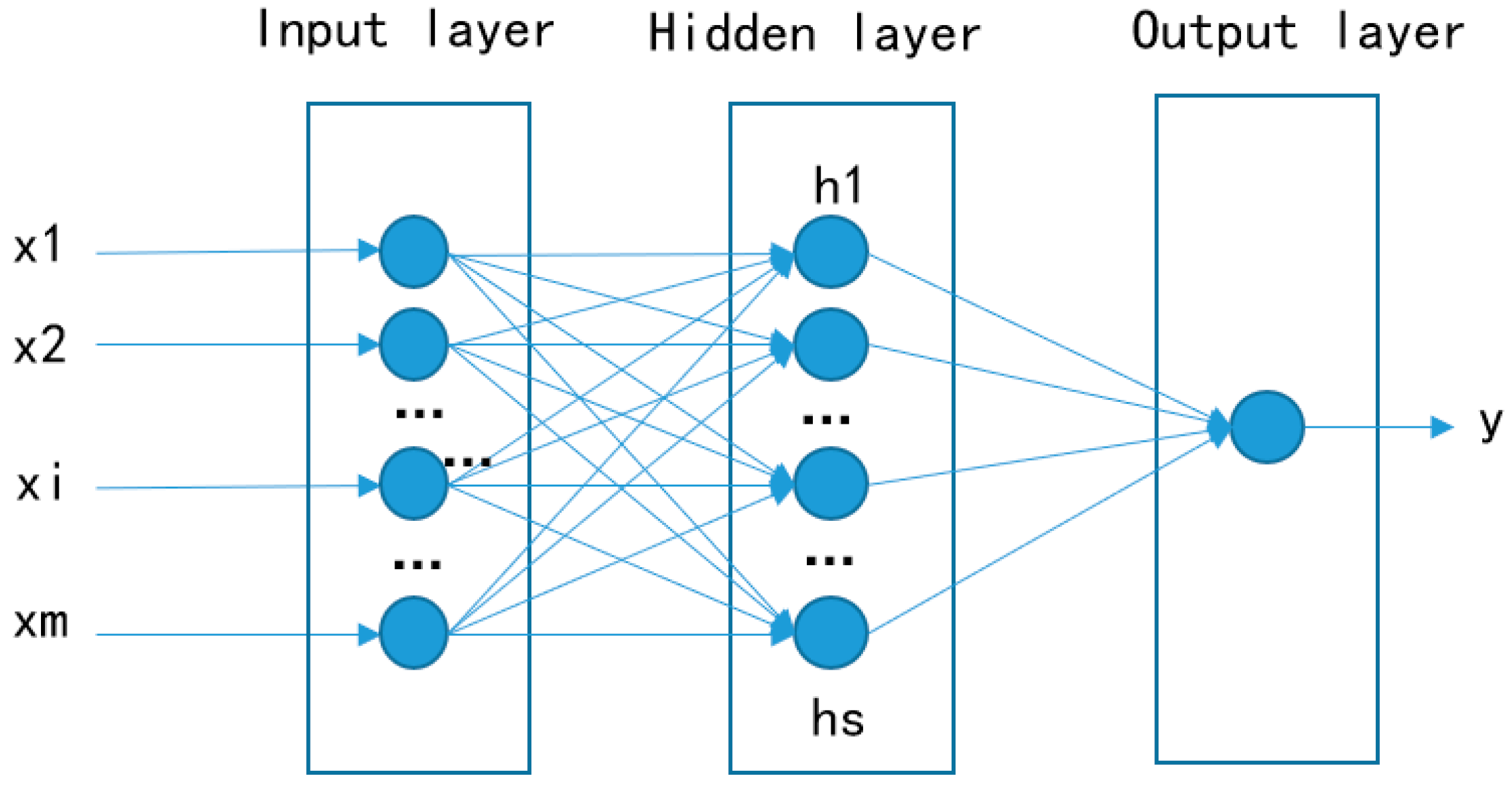
2.2.2. Selecting the Superior Ensemble Method from MLP, SVR, and RF

After data preprocessing, MLP, SVR, and RF methods were applied to the ensemble 21-model NEX-GDDP, and the performance of each method was compared. Then, the superior SVR method was selected. The applied methods have previously been successfully applied to modelling nonlinear relationships between local precipitation and GCM predictors [18] because they have the ability to model highly nonlinear relationships.
MLP is a typical neural network [31] with the back-propagation (BP) training algorithm [32]. In this study, a typical three-layer MLP network was used that consisted of one input layer, one hidden layer, and one output layer. Figure 2 depicts the construction of the applied MLP network. {x1,…xm,…xn} represents the PCs of NEX-GDDP precipitation, and y represents the corresponding observed data. {h1,…hs} denotes the nodes of the hidden layer.
Equation (1) describes the input–output equation of the applied MLP network in this study [33]:
y ^ = f o [ j = 1 M w j . f h ( i = 1 N w j i x i + w j o ) + w o ]
where w j i are the weights in the hidden layer that connect the i-th neuron in the input layer and the j-th neuron in the hidden layer, wjo is the bias for the j-th hidden neuron, f h is the activation function of the hidden neuron, w j is the weight between the j-th neuron in the hidden layer and the neuron in the output layer, w o is the bias for the output neuron, and f o is the activation function for the output.
SVM is also a machine learning method based on Vapnik–Chervonenkis (VC) theory and the rule of structural risk minimization [17]. SVR is the SVM that solves nonlinear regression problems by applying kernel functions to map the low-dimensional data to a high-dimensional feature space. SVR methods have been successfully applied in precipitation downscaling [34,35]. There are no documented applications for ensemble multiple NEX-GDDP precipitation. In this study, the applied SVR model can be represented by Equation (2):
y = f ( x ) = 1 z ( α i α i ^ ) K e r n e l x i , x + b
where K e r n e l   denotes the applied kernel function; α i and α i ^ denote Lagrange multipliers, which could achieve the optimization problem; b is a parameter; xi are vectors; and x is the independent vector. The parameters are derived by maximizing the objective function.
In addition, RF was proposed by Breiman [36] as a novel machine learning algorithm. It includes a multiple classification and regression decision tree (CART), which may avoid over-fitting and can adjust different types of input variables. For more detail on CART analysis, refer to Breiman et al. [37]. RF can generate many independent trees and then make a final decision on the basis of its characteristics of nonparametric statistical regression and randomness. Accordingly, the decision-making ability of the RF model hinges on each CART. Using out of bag (OOB), RF can be internally cross-validated. This study applied the OOB error ( E O O B ) to estimate the internal error, represented by Equation (3):
E O O B = 1 n i = 1 n [ Y ˜ ( X i ) Y i ] 2
where Y ˜ ( X i ) are the predicted values and Y i are the station observations. Regarding RF, the number of trees and the maximum depth of each tree are the main hyperparameters.
Note that the choice and determination of hyperparameters for machine learning methods is important; for example, for MLP, it is essential for the choice of the number of hidden layers and neurons, activation functions, optimal algorithms, and others [38]. For SVR, it is important for the penalty factor, toleration, and kernel function, and for RF, the number of trees and the maximum depth of each tree are important.
In this study, Bayesian hyperparameter optimization (BHO) was used to determine the hyperparameter choice of MLP, SVR, and RF ensemble models. The BHO can map the hyperparameters to the corresponding scoring probability of the objective (e.g., the MSE and loss of model performance) to infer information on the unknown function [39]. In this study, the tree-structured Parzen estimator (TPE) algorithm was chosen because it performed better for several difficult learning problems [40]. The framework of sequential model-based global optimization (SMBO) was also used in BHO. In addition, in the process of hyperparameter optimization, a 10-fold cross-validation was applied to promote more reliable results—the dataset during the historic period of 1961–2005 was divided into 10 equal-sized sub-datasets. There were 10 rounds of training and validation; each round used 9 out of the 10 sub-datasets as training data, and the remaining round was used for validation.
The software used to implement BHO for MLP, SVR, and RF is introduced in Appendix A. Figure A1 and Figure A2 in Appendix A depict the diagrams of the optimization process of the ML methods for the region mean. Table A1, Table A2 and Table A3 in Appendix B provide the results of BHO of MLP, SVR, and RF for each model.
All ML ensemble models were established on the basis of the optimal hyperparameters, whereas the selected PCs of 21 NEX-GDDP precipitation variables were used as inputs to the models and drove them to generate the ensemble precipitation corresponding to the stations. Then, on the basis of the evaluation metrics from Section 2.2.4, SVR was selected as the best ensemble method.

2.2.3. Combining the SVR and QM Methods

Precipitation bias still remains after ensemble simulation, and thus it is important to further reduce bias. QM has been successfully applied for many precipitation bias-corrected studies, and it is considered the most efficient method for the task [25,26]. After the selection among the MLP, SVR, and RF ensemble methods, this study combined the SVR methods for ensemble simulation and the QM method for bias correction on the basis of 21 NEX-GDDP precipitation models. QM is a distribution-based method that is always used to align the cumulative distribution function (CDF) of two data series [41]. Equation (4) describes the general form of QM:
P q = f s t a 1   ( f m   ( p m ) )
where P q is the corrected precipitation after quantile mapping, f s t a 1 is the inverse CDF corresponding to observed precipitation, f m denotes the CDF of ensemble-simulated data generated by SVR, and p m is the simulated data.
In this study, the employed QM technique was based on quantile–quantile (Q–Q) plots, which express the Q–Q relation of modelled and observed series. The Q–Q plot is regarded as an empirically based transfer function to align the percentiles of ensemble-simulated data and observations. This study determined the transfer function on the basis of historic precipitation and then applied the function to correct the simulation of future projections. The software and packages used to implement the QM method are introduced in Appendix C.

2.2.4. Evaluation and Projection for SVR_QM

The performance of raw NEX-GDDP models; MLP, SVR, and RF models; and SVR_QM models were all assessed by comparing the results with observations. In this study, three evaluation metrics were used, including Pearson’s correlation coefficient (PCC), root mean squared error (RMSE), and relative bias (Rbias), equations that are shown in Table 4. These metrics were also regarded as the indicators for the performance comparison of each method. PCC was used to evaluate the degree of linear correlation between variables; a PCC of 0 denotes no correlation whereas 1 represents complete correlation. RMSE represents the errors between two variables; the smaller the RMSE, the better the results. Rbias was used to evaluate the relative deviation between simulated and observed data.
The projected precipitation rates from 2006 to 2095, under RCP4.5 and RCP8.5, were assembled into an ensemble and corrected using the established SVR_QM models. In other words, the corresponding PCs were selected, and the established SVR and QM models were used to obtain the station’s future precipitation. Then, on the basis of the modelled results for the future, the yearly trends of precipitation changes were analyzed.

3. Results and Discussion

3.1. Validation and Comparison of the Machine Learning Ensemble Models

First, the MLP, SVR, and RF models have been used for ensemble simulations. For comparison, MME was used to ensemble the NEX-GDDP models, and the arithmetic mean of the precipitation values of the 21 models was used to yield an ensemble simulation.
Table 5 shows the simulation performance of the 21 single NEX-GDDP models and MME ensemble model for the region mean, including PCC, RMSE, and Rbias. Given space limitations, the evaluation results of each station are presented in Table S1 in the Supplementary Materials. Each model had a certain ability to simulate the observed precipitation, although the simulation ability of each model and the performance for each station-based single model was obviously different. Obviously, the models 2, 4, and 15 overall outperformed the other NEX-GDDP models because the PCC reached 0.68–0.72, and the RMSE reached approximately 43–45 mm, whereas the models 6, 17, and 20 had relatively poor performance as the PCC was 0.60–0.61 and the RMSE was approximately 50–52 mm. Figure 3 depicts the Taylor diagram of raw NEX-GDDP models, MME, and ML ensemble models, which could present the PCC, RMSE, and standard deviation of each model and the observations. Generally, the closer to the ‘observed’ point, the better the performance. It can be seen that there were more obvious conclusions that were consistent with the conclusions of Table 5. In addition, the standard deviations of these models were closed to the observation. It is interesting that the good PCCs were accompanied by poor RMSEs and Rbias values in several cases. Maybe this was because the system deviation of CMIP5 models greatly impact the values of RMSEs and Rbias. Moreover, regarding the different performance of each station, the simulation results of the 21 models of stations 1, 5, and 9 were relatively poor, whereas those of stations 17, 19, and 21 were good. This may have been due to the local microclimate that the GCMs could not consider. The microclimate was influenced by the local topography, underlying surface, and weather. Additionally, the statistical downscaling strategy of generating the NEX-GDDP from these GCMs also did not consider regional climate. This theme is worthy of further study, as the local conditions of each station are different. These results also confirm the definite simulation ability of NEX-GDDP models for some complex terrain areas, as is demonstrated by the similar conclusions of previous studies [10]. For MME, there were clear improvements for all single NEX-GDDP models. For the region mean, the PCC was improved from 0.60–0.72 to 0.75, and the RMSE was reduced to 36.68 mm. This result is also consistent with those of previous studies, although the cases and specific values are different [20].
Figure 4 depicts the PC numbers for each station, and the comparison of three ML ensemble methods for the performance evaluation is shown in Table 6. It can be seen that SVR overall performed better than MLP and RF for ensemble, as the PCC reached 0.81 and RMSE reached 34.24 mm for region mean, whereas the PCC of MLP and RF were 0.77 and 0.78, respectively, and RMSE were 35.78 and 36.21 mm. For 21 stations, the PCC of SVR reached 0.56–0.86, and RMSE reached 37.64–80.65 mm, which also performed better than MLP and RF. The results of stations 7, 14, and 18 were very good, whereas those of stations 1, 2, 3, and 9 were relatively bad. As concluded from Table 5 and Table 6, all the ML ensemble models showed greatly improved performance compared with the raw NEX-GDDP simulation and the results of MME, although the improvement degree for MME was not comparable to those for raw simulation. This situation may be because the MME ensemble was relatively good, which made significant improvement more difficult. A similar conclusion was confirmed in previous references, where SVR overall performed better than RF for GCM precipitation downscaling, although there were some opposite cases for specific stations [20]. However, it can be concluded that SVR was more reliable for the study area or the characteristics of used data. In future work, it is worth studying the applicability of SVR for other regions or basins. For the different results of specific stations, this was also perhaps because the influences of the unconsidered local climates of some stations were significant. Although the ML methods have been popularly applied, they were first used for the ensemble NEX-GDDP precipitation. The results in this study demonstrated that there were relative uncertainties among the three ML ensemble methods. Generally, the modelling performance of the ML methods depends on their inputs and parameters [42]. It is difficult to improve the raw quality of NEX-GDDP. However, for the parameter set, there may be room for improvement by improving the ML algorithm and optimizing BHO. Satisfactory research has applied the ensemble multi-method strategy to reduce the uncertainties [43], which has inspired further studies to apply more ensemble methods and obtain the best method that is more applicable at the method aspect.

3.2. Validation of SVR_QM Method

According to Section 3.1, the SVR models performed best overall for the ensemble simulation of NEX-GDDP precipitation in this region. This study further applied the QM method to correct the results of the SVR models. According to Equation (4), the ensemble result from SVR was regarded as the simulated data, P m whereas f s t a 1 is the inverse CDF corresponding to observed precipitation.
Table 7 shows the results of SVR_QM models for each station and region mean. Satisfied results were shown in most stations, as the PCC was up to 0.58–0.85 and RMSE approximately reached to 37–80 mm for 21 stations. The performance for stations 1 and 3 were still relatively poor, whereas the results for stations 7, 14, and 18 were good. As for region mean, the PCC and RMSE reached 0.84 and 33.78 mm, respectively. More obviously, the Rbias were improved when compared with the results of ML methods and MME. Table 8 shows the comparison of MME, MLP, SVR, RF, and SVR_QM for the region mean. SVR_QM had the superior performance from Table 6, Table 7 and Table 8, and although the improvement of PCC and RMSE was not obvious, Rbias was almost eliminated for all cases. The Rbias obtained from SVR_QM reached −0.04% for the region mean, whereas the values obtained from MME, MLP, SVR, and RF were 2.23%, −1.82%, −2.48%, and −2.21%. This may have been mainly due to certain defects of data quality; it is difficult to improve the PCC and RMSE when data are to some extent defective. As the CMIP6 is ongoing, more reliable GCM data may be released in the future. There are great expectations for the improvement of correction accuracy on the basis of the new dataset. Figure 5 depicts the scatter plots between the monthly SVR_QM results and the observations for each station and the region mean in the period of 1961–2005. The horizontal axes show the observed precipitation, whereas the vertical axes show the SVR_QM results. The blue line represents the line of function ‘y = x’. The more concentrated the scatter on the line, the closer the simulation to observations. Clearly, the degrees of concentration were different among all stations. The region mean was the most concentrated one, and stations 7 and 18 were more concentrated than other stations, whereas stations 1 and 3 were less concentrated. In conclusion, it was demonstrated that the simulation performance generated from SVR_QM had been improved, but some stations still exhibited relatively poor performance. These results also inspire the exploration of the influence of local climate or topography in the future.
The QM method has been proven to have a certain ability to correct NEX-GDDP precipitation because consistent conclusions were also reached for GCM precipitation cases [7]. However, from Raghavan et al., the raw simulation of daily NEX-GDDP precipitation is poor [11]. It is worth attempting to apply the same framework for daily NEX-GDDP precipitation, which could prompt more reliable revelation of extreme rainfall and weather in the future, given the lack of research.

3.3. Projected Precipitation in the Han River Basin during the 21st Century under RCP4.5 and 8.5

The monthly rainfall simulation was converted to annual time series. The non-parametric Mann–Kendall method [44,45,46] was used to detect future trends of yearly precipitation. Trends were tested at three significance levels of α = 0.10, 0.05, 0.01 (the |Z| was greater than 1.28, 1.64, and 2.32). Table 9 presents the changing trend and calculated values of Z of annual timescales of future precipitation for each station and region mean in the period of 2006–2095 under RCP4.5 and RCP8.5. From the table, it is implied that there are increasing trends among most stations under RCP4.5 and RCP8.5, as the corresponding precipitation series had positive trend values. In addition, these increasing cases almost had a significant trend, as the Z values were greater than 1.28. Under RCP4.5, the stations 9, 11, and 15 showed the most significantly increasing trend, as the Z values were up to 2.62, 3.31, and 3.58, respectively, whereas stations 10 and 18 showed a non-significantly increasing trend, as the Z values were 1.23 and 0.44, respectively. Under RCP8.5, the stations 9, 15, and 21 showed the most significantly increasing trend, as the Z values were up to 4.14, 4.94, and 4.21, respectively, whereas stations 5 and 10 showed a non-significantly increasing trend. For these increasing cases, the trend significance of RCP8.5 was higher than RCP4.5. In addition, there were less cases which showed a decreasing trend, such as stations 2, 5, 6, 7, 12, and 15 under RCP4.5, and stations 2 and 6 under RCP8.5. The trend differences of these stations may have been due to the difference of local climate. It is interesting to explore the relationship between the changing trend of climate and the local climate in the future study. In addition, for region mean, the increasing trends were very significant under RCP4.5 and RCP8.5, whose increasing trends were 0.58 and 0.85 mm/year, respectively, and Z values were up to 4.34 and 7.43, respectively.
Assuming 1981–2000 as the historical baseline, Table 10 shows the changes of precipitation in the future compared with baseline years for each station and the region mean. The average rainfall during the middle (2040–2059) and late (2070–2089) 21st century was shown to increase by 3.54% and 5.12%, respectively, compared with the base years under RCP4.5, and they were shown to increase by 7.44% and 9.52% under RCP8.5, respectively. Most station cases showed the increase trend as the value reached 0.13% to 23.89%. Under RCP4.5 and RCP8.5, stations 6, 7, and 8 showed the biggest increase in change, whereas stations 1, 2, 14, and 16 showed the smallest increase in change. In addition, there were some decreasing cases during the middle and late 21st century, especially under RCP4.5. These differences may have been due to the raw data, model uncertainty, and local climate. In the future, the uncertainty of future projection should be explored and alleviated.
Figure 6 shows the changes of projected future annual precipitation in the Han River basin. Under RCP4.5, it can be seen that the rainfall during the 21st century is shown to have a weakly overall increasing trend and that there was shown to be a slight downward fluctuation, weakly increasing trend, and obviously increasing trend in the periods of 2005–2040, 2041–2059, and 2070–2089, respectively. Under RCP8.5, the increase of precipitation was shown to be more significant after 2040, and there were several years which were shown to have heavy rainfall, such as 2070 and 2089. This is also a valuable topic to study the year of heavy rainfall. Figure 7 compares the statistics of the historical baseline and the middle and late 21st century time series on the basis of quantile–quantile plots under RCP4.5 and RCP8.5. It can be seen that most rain distributions were near the normal distributions. In each sub-figure, three baselines that represented the corresponding normal distributions are shown. The interception and slope of these lines represent the mean and variance, respectively. Compared with the period of 1981–2000, the average precipitation of the mid and late 21st century under RCP4.5 and RCP8.5 were shown to clearly increase, and the variances were also shown to be different.
The trend of annual precipitation was shown to change in the 21st century in the Han River Basin and was coincident with those of previous studies, although the specific results were not the same [47,48]. This conclusion is acceptable because the data used and study strategies were different. There may be obvious seasonality, although no measures were taken to eliminate it in this study. Therefore, the projection of seasonal rainfall may have more uncertainties. There are several studies that separately implemented training ensemble models according to each calendar season or month [49]. This study considered a sufficient number of samples for the training of the SVR methods and thus used whole monthly data for modelling. It is a feasible strategy for this study to study the changes of individual season or month in the 21st century, which would conclude the solution exploration for the barrier of seasonality of rainfall and insufficient samples.
There are further plans to train monthly and seasonal models on the basis of daily data, although much uncertainty exists in the daily rainfall. Some successful studies have assessed extreme precipitation events on the basis of daily downscaled precipitation [50]. It is also worth studying daily precipitation on the basis of NEX-GDDP models in future work.

4. Conclusions

It is important to know the future climate change at the local scale in the Han River basin. Benefitting from the release of the high-resolution downscaled NEX-GDDP dataset, there are many ways to make use of it for studying the simulation and projection of local climate. This study first compared the abilities of three ML methods (MLP, SVR, and RF) for ensemble simulation of 21 NEX-GDDP precipitation models for the historic years of 1961–2005, with MME applied as a reference. Then, on the basis of the results of the SVR models, this study used the QM method to correct the ensemble series. Finally, the SVR_QM ensemble and correction models were applied to project the change of precipitation in the period of 2006–2095 under RCP4.5 and RCP8.5 in this region. Several statistical metrics (PCC, RMSE, Rbias) were used to evaluate and compare the performance of each method. The conclusions were as follows:
(1)
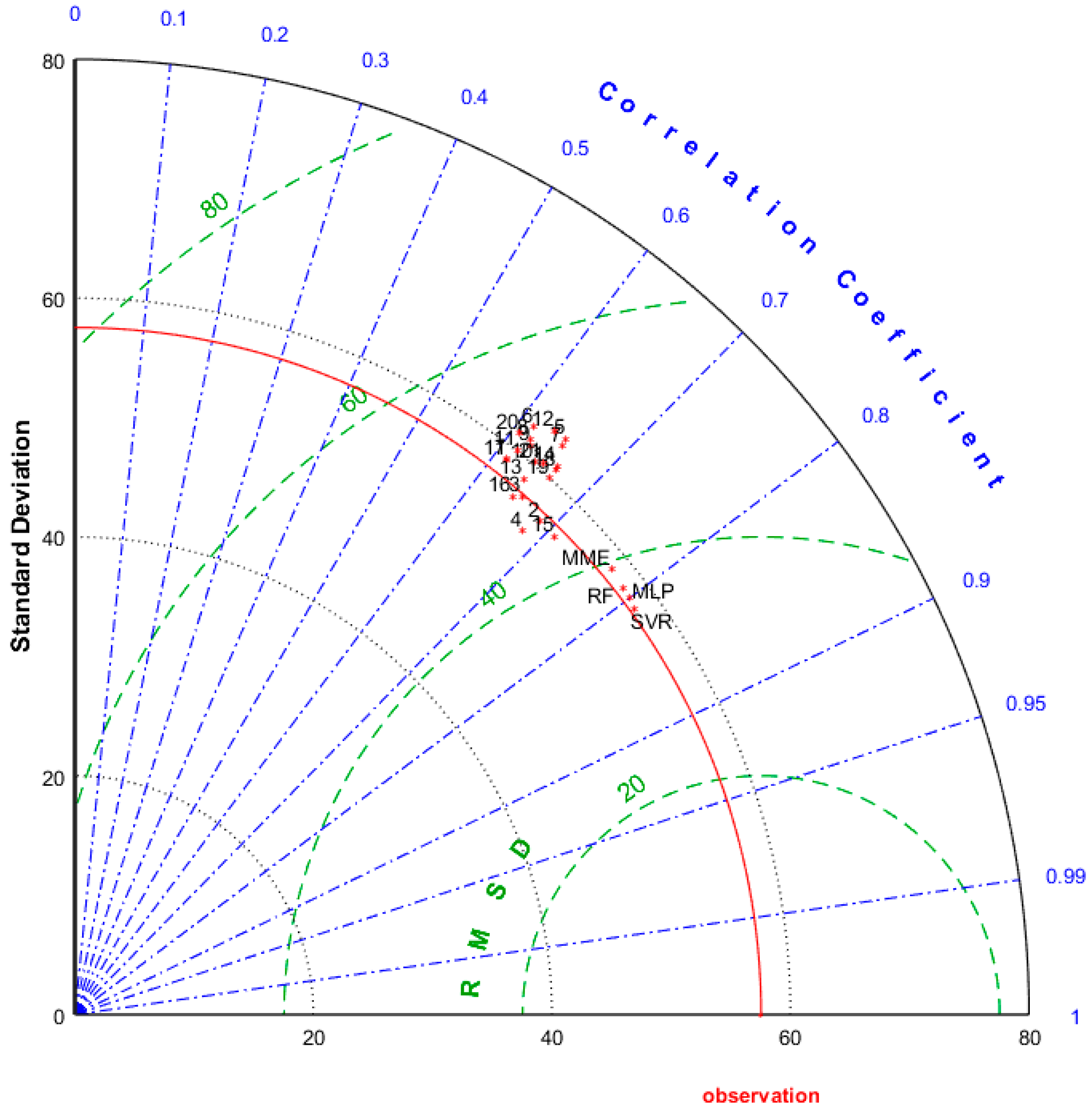
The raw precipitation simulation of individual NEX-GDDP models had a certain reliability for the Han River basin—the PCC was 0.61–0.71, and RMSE was approximately 48–51 mm. The results of three ML methods and MME all demonstrated their superiority over all individual NEX-GDDP models—the PCC improved to 0.77–0.81, and RMSE was 34–37 mm. The ML performed better than MME. Overall, the SVR showed the best performance—PCC was up to 0.81, and RMSE was up to 34.52 mm. For each station, there were similar conclusions on the whole, although there were less contrary ones for several stations. However, the different performance of each station was obvious. This may have been due to the influence of the raw data, model uncertainty, and especially the local climate.
(2)
The application of the QM method for the results of SVR models demonstrated the further improvement of the simulation reliability. Although there were some improvements for PCC and RMSE, Rbias was obviously alleviated compared with MME, MLP, SVR, and RF. The Rbias values were reduced to −2.04–0.36% for each station and −0.04% for the region mean. The best models established on the basis of historic series could improve the reliability of projected precipitation.
(3)
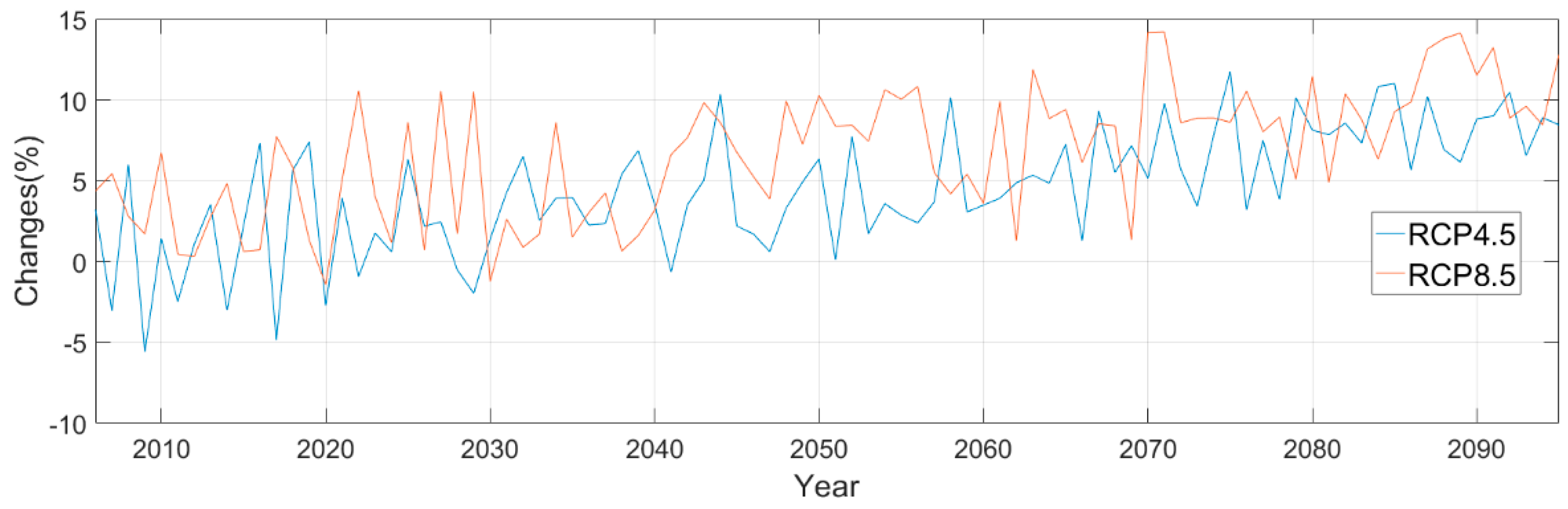
The changes of precipitation during the 21st century in this region had a very significantly increasing trend under RCP4.5 and RCP8.5, whereas there was a slight decreasing fluctuation in the period of 2006–2040. More specifically, compared with the base years, the regional average precipitation during the middle and late 21st century increased by 3.54% and 5.12% under RCP45 and by 7.44% and 9.52% under RCP8.5, respectively. In addition, it can be concluded that the increasing trends existed among most stations under RCP4.5 and RCP8.5, and most of these cases were also significant. These results were expected to be used for the guidance of more accurate long-term management strategies such as water resource allocation, flood mitigation, and ecological layout, among others.
This study first developed SVR_QM ensemble and correction models for NEX-GDDP data in the Han River basin and generated preliminary projections of changes of precipitation during the 21st century for the region, obtaining relatively satisfied results. However, there were some unsolved problems. It may be worthwhile for this study to further explore the improvement of study methods and integrate the influence of local factors, with a subsequent study of the daily datasets of NEX-GDDP.

Supplementary Materials

The following are available online at https://www.mdpi.com/2073-4433/10/11/688/s1, Table S1: The evaluation of 21 NEX-GDDP models and MME for specific stations in this region.

Author Contributions

Conceptualization, Z.C. and Y.C.; validation and investigation, R.X.; methodology, Z.C., Y.C. and R.X.; software, Z.C., Y.C. and R.X.; writing—Original draft preparation, R.X.; writing—Review and editing, Z.C. and Y.C.; project administration and funding acquisition, Z.C. and Y.C.

Funding

This work was supported by the National Key Research and Development Program of China (No. 2017YFB0503704), the National Nature Science Foundation of China program (No. 41671380, 41771422, 41890822)

Acknowledgments

We give thanks to the free data from the China Meteorological Administration (http://data.cma.cn/) and NASA (https://nex.nasa.gov/nex/projects/1356/).

Conflicts of Interest

The authors declare no conflict of interest.

Appendix A

This section discusses the used software for hyperparameter optimization, and presents the diagrams of the optimization process of MLP, RF, and SVR methods for the region mean.
This study used Python’s ‘hyperopt’ package to implementing BHO for MLP and RF, and MATLAB’s ‘fitrsvm’ function for SVM because it is a self-contained function in MATLAB 2016b. The mean squared error (MSE) was regarded as the validation score (objective) for ML and RF, and the self-contained function of ‘fitrsvm’, and the loss function was deemed as the objective for SVR.
Figure A1. Bayesian hyper-parameter optimization process of (a)MLP and (b)RF ensemble modelling.
Atmosphere 10 00688 g0a1
Figure A2. Bayesian hyper-parameter optimization process of SVR ensemble modelling.
Atmosphere 10 00688 g0a2

Appendix B

This section presents the results of BHO of MLP, SVR, and RF for each model.
Table A1. Optimal results of Bayesian hyper-parameter optimization for MLP for this region.
ActivationAlphaHLZLRMax_IterSolverTolerationObjective
1logistic0.3889321invscaling1716adam0.00947159
2logistic9.3682225adaptive1746sgd0.0085044603
3logistic3.20823219constant1662adam0.0012925616
4relu8.77100928adaptive1365adam0.003823510
5tanh9.89762322adaptive1073sgd0.0036724105
6tanh9.63757924adaptive1928adam0.0032422627
7relu3.9434128constant122sgd0.0077661748
8tanh9.51567217invscaling1880adam0.009963413
9logistic9.64830522constant1333adam0.0085672920
10logistic9.502818constant740sgd0.0009712241
11logistic1.62297919invscaling1570adam0.0055832376
12relu5.24133425constant1731adam0.0091183236
13tanh5.08516721adaptive1552sgd0.0058052862
14logistic8.69528524adaptive114sgd0.0089184095
15relu5.98171113constant1868adam0.0082982793
16tanh5.29904129constant1843adam0.0019892168
17relu5.8159220adaptive1462adam0.0020422847
18relu2.62384915invscaling1973sgd0.0055372729
19tanh9.00335921adaptive1520adam0.0059042825
20tanh9.22040225invscaling1140adam0.0070811659
21tanh2.95073123adaptive1278sgd0.0027211790
meantanh4.39405517invscaling1006sgd0.0014511288
* HLZ denotes hidden_layer_sizes; LR denotes learning_rate.
Table A2. Optimal results of Bayesian hyper-parameter optimization for RF in this region.
Max_DepthMax_FeaturesN_EstimatorsObjective
168556870
2454294634
378875486
4583763589
5785474044
61053142562
71174741735
8184913456
91544352878
10116562292
11572262360
12761463265
131451443012
141741224306
151343712888
16573122238
17782192883
18782662770
191144662808
201473111673
21118901762
mean168951304
Table A3. Optimal results of Bayesian hyper-parameter optimization of SVR in this region.
StationBox ConstraintKernel ScaleEpsilonKernel FunctionPolynomial OrderStandardizeObjective
144.83156.480.48647GaussianNaNfalse8.6212
2112.8770.4452.3872GaussianNaNfalse8.1288
383.342112.340.3045GaussianNaNfalse8.1611
489.15728.7090.089533GaussianNaNfalse8.3211
522.73419.5740.48647GaussianNaNtrue7.8536
6103.68NaN0.8746Polynomial (rbf)2true7.4314
7203.68NaN0.30124Polynomial (rbf)2true7.406
8353.41124.2230.33471gaussianNaNtrue7.9878
918.997NaN2.8774Polynomial2true7.6882
10332.85NaN1.38503Polynomial2True7.7515
1178.67950.4320.8879GaussianNaNfalse8.0716
12189.78155.841.8994GaussianNaNtrue7.9665
13263.568.18460.054217gaussianNaNtrue8.3216
14247.2288.69110.54884gaussianNaNtrue7.9045
15371.78102.87220.04587gaussianNaNtrue7.9458
16167.8823.6850.1066gaussianNaNtrue7.6972
1753.2973.63860.75566gaussianNaNfalse7.9461
18594.1627.8980.38872gaussianNaNfalse7.8806
19288.76NaN0.78661Polynomial2True7.8977
20610.8732.5381.6156gaussianNaNfalse7.4072
21412.66NaN1.1667Polynomial2True7.5092
mean305.4645.0251.0788gaussianNaNtrue7.1463
* NAN denotes ‘Not a Number’.

Appendix C

This section discusses the used software for the achievement of QM methods.
In this study, two functions in the ‘qmap’ package in R3.6.0 were used. One was the function ‘fitQmapRQUANT’, which was used to estimate the values of the Q–Q relation between observed and simulated data on the basis of local linear least square regression, and the other was the ‘doQmapRQUANT’ function, which could implement QM by interpolating the empirical quantiles.

References

  1. Mann, M.E.; Rahmstorf, S.; Kornhuber, K.; Steinman, B.A.; Miller, S.K.; Coumou, D. Influence of anthropogenic climate change on planetary wave resonance and extreme weather events. Sci. Rep. 2017, 7, 45242. [Google Scholar] [CrossRef] [PubMed]
  2. Naveendrakumar, G.; Vithanage, M.; Kwon, H.H.; Chandrasekara, S.S.K.; Iqbal, M.C.M.; Pathmarajah, S.; Obeysekera, J. South Asian perspective on temperature and rainfall extremes: A review. Atmos. Res. 2019, 225, 110–120. [Google Scholar] [CrossRef]
  3. Moncrieff, M.W.; Liu, C.; Bogenschutz, P. Simulation, modeling, and dynamically based parameterization of organized tropical convection for global climate models. J. Atmos. Sci. 2017, 74, 1363–1380. [Google Scholar] [CrossRef]
  4. Farjad, B.; Gupta, A.; Sartipizadeh, H.; Cannon, A.J. A novel approach for selecting extreme climate change scenarios for climate change impact studies. Sci. Total Environ. 2019, 678, 476–485. [Google Scholar] [CrossRef] [PubMed]
  5. Abbasian, M.; Moghim, S.; Abrishamchi, A. Performance of the general circulation models in simulating temperature and precipitation over Iran. Theor. Appl. Climatol. 2019, 135, 1465–1483. [Google Scholar] [CrossRef]
  6. Rashid, M.; Jia, S.F.; Nitin, K.T.; Sangam, S. Precipitation Extended Linear Scaling Method for Correcting GCM Precipitation and Its Evaluation and Implication in the Transboundary Jhelum River Basin. Atmosphere 2018, 9, 160. [Google Scholar] [CrossRef]
  7. Yhang, Y.B.; Sohn, S.J.; Jung, I.W. Application of Dynamical and Statistical Downscaling to East Asian Summer Precipitation for Finely Resolved Datasets. Adv. Meteorol. 2017, 2017, 2956373. [Google Scholar] [CrossRef]
  8. Shin, Y.; Yi, C. Statistical Downscaling of Urban-scale Air Temperatures Using an Analog Model Output Statistics Technique. Atmosphere 2019, 10, 427. [Google Scholar] [CrossRef]
  9. Jain, S.; Salunke, P.; Mishra, S.K. Advantage of NEX-GDDP over CMIP5 and CORDEX Data: Indian Summer Monsoon. Atmos. Sci. 2019, 228, 152–160. [Google Scholar] [CrossRef]
  10. Chen, H.P.; Sun, J.Q.; Li, H.X. Future changes in precipitation extremes over China using the NEX-GDDP high-resolution daily downscaled data-set. Atmos. Ocean. Sci. Lett. 2017, 10, 403–410. [Google Scholar] [CrossRef] [Green Version]
  11. Raghavan, S.V.; Hur, J.; Liong, S.Y. Evaluations of NASA NEX-GDDP data over Southeast Asia: Present and future climates. Clim. Chang. 2018, 148, 503–518. [Google Scholar] [CrossRef]
  12. Knutti, R.; Furrer, R.; Tebaldi, C.; Cermak, J.; Meehl, G.A. Challenges in Combining Projections from Multiple Climate Models. J. Clim. 2010, 23, 2739–2758. [Google Scholar] [CrossRef] [Green Version]
  13. Tebaldi, C.; Smith, R.L.; Nychka, D. Quantifying uncertainty in projections of regional climate change: A Bayesian approach to the analysis of multimodel ensembles. J. Clim. 2005, 18, 1524–1540. [Google Scholar] [CrossRef]
  14. Li, J.; Yang, Y.M.; Wang, B. Evaluation of NESMv3 and CMIP5 Models’ Performance on Simulation of Asian-Australian Monsoon. Atmosphere 2018, 9, 327. [Google Scholar] [CrossRef]
  15. Mosavi, A.; Ozturk, P.; Chau, K.W. Flood Prediction Using Machine Learning Models: Literature Review. Water 2018, 10, 1536. [Google Scholar] [CrossRef]
  16. Ochoa, A.; Campozano, L.; S´anchez, E.; Gual´an, R.; Samaniego, E. Evaluation of downscaled estimates of monthly temperature and precipitation for a Southern Ecuador case study. Int. J. Climatol. 2015, 36, 1244–1255. [Google Scholar] [CrossRef] [Green Version]
  17. Vapnik, V. The Nature of Statistical Learning Theory, 2nd ed.; Information Science and Statistics; Springer-Verlag: New York, NY, USA, 2000; ISBN 978-0-387-98780-4. [Google Scholar]
  18. Sachindra, D.A.; Ahmed, K.; Rashid, M.M.; Shahid, S.; Perera, B.J.C. Statistical downscaling of precipitation using machine learning techniques. Atmos. Res. 2018, 212, 240–258. [Google Scholar] [CrossRef]
  19. Najafi, M.R.; Moradkhani, H.; Wherry, S.A. Statistical Downscaling of Precipitation Using Machine Learning with Optimal Predictor Selection. J. Hydrol. Eng. 2011, 16, 650–664. [Google Scholar] [CrossRef]
  20. Sa’adi, Z.; Shahid, S.; Chung, E.S.; Ismail, T.B. Projection of spatial and temporal changes of rainfall in Sarawak of Borneo Island using statistical downscaling of CMIP5 models. Atmos. Res. 2017, 197, 446–460. [Google Scholar] [CrossRef]
  21. Rashid, M.; Beecham, S.; Chowdhury, R. Simulation of extreme rainfall from CMIP5 in the Onkaparinga catchment using a generalized linear model. In Proceedings of the MODSIM2013, 20th International Congress on Modelling and Simulation. Modelling and Simulation Society of Australia and New Zealand, Adelaide, Australia, 1–6 December 2013; pp. 2520–2526. [Google Scholar]
  22. Rashid, M.M.; Beechama, S.; Chowdhury, R.K. Statistical downscaling of CMIP5 outputs for projecting future changes in rainfall in the Onkaparinga catchment. Sci. Total Environ. 2015, 530–531, 171–182. [Google Scholar] [CrossRef]
  23. Xu, L.; Chen, N.C.; Zhang, X.; Chen, Z.Q.; Hu, C.L.; Wang, C. Improving the North American multi-model ensemble (NMME) precipitation forecasts at local areas using wavelet and machine learning. Clim. Dyn. 2019, 53, 601–615. [Google Scholar] [CrossRef]
  24. Shukla, A.K.; Ojha, C.S.P.; Singh, R.P.; Pal, L.; Fu, D.F. Evaluation of TRMM Precipitation Dataset over Himalayan Catchment: The Upper Ganga Basin, India. Water 2019, 11, 613. [Google Scholar] [CrossRef]
  25. Hamill, T.M.; Scheuerer, M. Probabilistic Precipitation Forecast Postprocessing Using Quantile Mapping and Rank-Weighted Best-Member Dressing. Mon. Weather Rev. 2018, 164, 4079–4098. [Google Scholar] [CrossRef]
  26. Themeßl, M.J.; Gobiet, A.; Leuprecht, A. Empirical-statistical downscaling and error correction of daily precipitation from regional climate models. Int. J. Climatol. 2011, 31, 1530–1544. [Google Scholar] [CrossRef]
  27. The Website of China Meteorological Data. Available online: http://data.cma.cn/ (accessed on 12 February 2019).
  28. Thrasher, B.; Xiong, J.; Wang, W.; Melton, F.; Michaelis, A.; Nemani, R. Downscaled Climate Projections Suitable for Resource Management. Eos Trans. Am. Geophys. Union 2011, 94, 321–323. [Google Scholar] [CrossRef]
  29. The Website of NEX Global Daily Downscaled Climate Projections. Available online: https://nex.nasa.gov/nex/projects/1356/ (accessed on 22 March 2019).
  30. Hotelling, H. Analysis of a Complex of Statistical Variables into Principal Components. J. Educ. Psychol. 1993, 24, 417. [Google Scholar] [CrossRef]
  31. Minsky, M.; Seymour, P. Perceptron: An Introduction to Computational Geometry; The MIT Press: Cambridge, MA, USA, 1969; Volume 88, p. 2. [Google Scholar]
  32. Rumelhart, D.E.; Geoffrey, E.H.; Ronald, J.W. Learning Internal Representations by Error Propagation; No. ICS-8506; California Univ San Diego La Jolla Inst for Cognitive Science: La Jolla, CA, USA, 1985. [Google Scholar]
  33. Kim, T.W.; Valdés, J.B. Nonlinear Model for Drought Forecasting Based on a Conjunction of Wavelet Transforms and Neural Networks. J. Hydrol. Eng. 2003, 8, 319–328. [Google Scholar] [CrossRef] [Green Version]
  34. Tripathi, S.; Srinivas, V.V.; Nanjundiah, R.S. Dowinscaling of precipitation for climate change scenarios: A support vector machine approach. J. Hydrol. 2006, 330, 621–640. [Google Scholar] [CrossRef]
  35. Pour, S.H.; Shahid, S.; Chung, E.S.; Wang, X.J. Model output statistics downscaling using support vector machine for the projection of spatial and temporal changes in rainfall of Bangladesh. Atmos. Res. 2018, 213, 149–162. [Google Scholar] [CrossRef]
  36. Breiman, L. Random Forests. Mach. Learn. 2001, 45, 5–32. [Google Scholar] [CrossRef] [Green Version]
  37. Breiman, L.; Friedman, J.; Stone, C.J.; Olshen, R.A. Classification and Regression Trees; CRC Press: Borarton, FL, USA, 1984. [Google Scholar]
  38. Maier, H.R.; Dandy, G.C. Neural networks for the prediction and forecasting of water resources variables: A review of modelling issues and applications. Environ. Model. Softw. 2000, 15, 101–124. [Google Scholar] [CrossRef]
  39. Xia, Y.F.; Liu, C.Z.; Li, Y.Y.; Liu, N.N. A boosted decision tree approach using Bayesian hyper-parameter optimization for credit scoring. Expert Syst. Appl. 2017, 78, 225–241. [Google Scholar] [CrossRef]
  40. Bergstra, J.S.; Bardenet, R.; Bengio, Y.; Kégl, B. Algorithms for hyper-parameter optimization. In Advances in Neural Information Processing Systems; Mit Press: Cambridge, MA, USA, 2011; pp. 2546–2554. [Google Scholar]
  41. Cannon, A.J.; Sobie, S.R.; Murdock, T.Q. Bias Correction of GCM Precipitation by Quantile Mapping: How Well Do Methods Preserve Changes in Quantiles and Extremes? J. Clim. 2015, 28, 6938–6959. [Google Scholar] [CrossRef]
  42. Whan, K.; Schmeits, M.C. Comparing Area Probability Forecasts of (Extreme) Local Precipitation Using Parametric and Machine Learning Statistical Postprocessing Methods. Mon. Weather Rev. 2018, 146, 3651–3673. [Google Scholar] [CrossRef]
  43. Wang, W.G.; Ding, Y.M.; Shao, Q.X.; Xu, J.Z.; Jiao, X.Y.; Luo, Y.F.; Yu, Z.B. Bayesian multi-model projection of irrigation requirement and water use efficiency in three typical rice plantation region of China based on CMIP5. Agric. For. Meteorol. 2017, 232, 89–105. [Google Scholar] [CrossRef]
  44. Mann, H. Non-parametric tests against trend. Econometrica 1945, 13, 245–259. [Google Scholar] [CrossRef]
  45. Kendall, M. Rank Correlation Methods, 4th ed.; Charles Griffin& Co. Ltd.: London, UK, 1975. [Google Scholar]
  46. Dinpashoh, Y.; Jahanbakhsh-Asl, S.; Rasouli, A.A.; Foroughi, M.; Singh, V.P. Impact of climate change on potential evapotranspiration (case study: West and NW of Iran). Theor. Appl. Climatol. 2019, 136, 185. [Google Scholar] [CrossRef]
  47. Kang, B.; Moon, S. Regional hydroclimatic projection using an coupled composite downscaling model with statistical bias corrector. KSCE J. Civ. Eng. 2017, 21, 2991–3002. [Google Scholar] [CrossRef]
  48. Ding, Y.M.; Wang, W.G.; Song, R.M.; Shao, Q.X.; Jiao, X.Y.; Xing, W.Q. Modeling spatial and temporal variability of the impact of climate change on rice irrigation water requirements in the middle and lower reaches of the Yangtze River, China. Agric. Water Manag. 2017, 193, 89–101. [Google Scholar] [CrossRef]
  49. Raziei, T. An analysis of daily and monthly precipitation seasonality and regimes in Iran and the associated changes in 1951–2014. Theor. Appl. Climatol. 2018, 134, 913–934. [Google Scholar] [CrossRef]
  50. Moron, V.; Robertson, A.W.; Ward, M.N.; Ndiaye, O. Weather types and rainfall over Senegal. Part II: Downscaling of GCM simulations. J. Clim. 2008, 21, 288–307. [Google Scholar] [CrossRef]
Figure 1. Han River system, altitudes, and station distribution.
Atmosphere 10 00688 g001
Figure 2. Construction of applied multi-layer perceptron (MLP) in this study.
Atmosphere 10 00688 g002
Figure 3. Taylor diagram of single NEX-GDDP models, MME, and machine learning (ML) ensemble models.
Atmosphere 10 00688 g003
Figure 4. Size of selected principal components (PCs) for each station and the region mean.
Atmosphere 10 00688 g004
Figure 5. Scatter plots between the SVR_QM results and the monthly observations for each station (au) and the region mean (v) in the period of 1961–2005. Horizontal axes show observed precipitation, and vertical axes show the SVR_QM results.
Atmosphere 10 00688 g005
Figure 6. Yearly changes of project precipitation under RCP4.5 and RCP8.5 compared to baseline year (1981–2000).
Atmosphere 10 00688 g006
Figure 7. Quantile–quantile plots of annual historic and projected precipitation under: (a) RCP4.5; (b) RCP8.5, respectively.
Atmosphere 10 00688 g007
Table 1. Location information of meteorological stations.
StationSignNumberLongitudeLatitudeElevation (m)
Taibai57,0281107.1934.021543.6
Liuba57,1242106.5633.381032.1
Hanzhong57,1273107.0233.04509.5
Foping57,1344107.5933.31827.2.
Nanxian57,1435109.5833.52742.2.
Zhenan57,1446109.0933.26693.7.
Shangnan57,1547110.5433.32523
Xishan57,1568111.333.18250.3
Nanyang57,1789112.2933.06129.2
Shiquan57,23210108.1633.03484.9
Ankang57,24511109.0232.43290.8
Yunxi57,25112110.2533249.1
Fangxian57,25913110.4532.03426.9
LaoHekou57,26514111.4432.2690
Xiangfan57,27815112.053268.6
Zaoyang57,27916112.4532.09125.5
Zhongxiang57,37817112.3431.165.8
Suizhou57,38118113.231.37116.3
Xiaogan57,48219113.5730.5425.5
Tianmen57,48320113.0830.431.9
Wuhan57,49421114.0330.3623.6
Luonan57,057\110.0934.06963.4
Zhumadian57,290\113.5532.5682.7
Baofeng57,181\113.0333.53136.4
Wugong57,034\108.1334.15447.8
Zhenping57,343\109.3231.54995.8
Xingshan57,359\110.4431.21336.8
Zhenba57,238\107.5432.32693.9
Ningqiang57,211\106.1532.5836.1
Table 2. Description of Representative Concentration Pathway RCP4.5 and RCP8.5.
RCPDescription
RCP4.5Radiative forcing increased to 4.5 W/m2 (~650 ppm CO2 -eq) by 2100
RCP8.5Radiative forcing is stable at 8.5 W/m2 (~1370 ppm CO2 -eq) by 2100
Table 3. Information about the 21 Coupled Model Intercomparison Project 5 (CMIP5) general circulation models (GCMs).
ModelNumberCountry and Institution
ACCESS1-01Commonwealth Scientific and Industrial Research Organization and Bureau of Meteorology, Australia
BCC-CMS1-12Beijing Climate Center, China
BNU-ESM3Institute of global change and Earth System Sciences, Beijing Normal University, China
CanESM24Canadian Centre for Climate Modelling and Analysis, Canada
CCSM45National Center for Atmospheric Research, America
CESM1-BGC6National Center for Atmospheric Research, America
CNRM-CM57Centre National de Recherches Meteorologiques, Centre Europeen de Recherche et Formation Avancees en Calcul Scientifique, France
CSIRO-Mk3-6-08Commonwealth Scientific and Industrial Research Organization/Queensland Climate Change Centre of Excellence, Australia
GFDL-CM39Geophysical Fluid Dynamics Laboratory, America
GFDL-ESM2G10Geophysical Fluid Dynamics Laboratory, America
GFDL-ESM2M11Geophysical Fluid Dynamics Laboratory, America
INMCM412Institute of Numerical Calculation, Russia
IPSL-CM5A-LR13Institut Pierre-Simon Laplace, France
IPSL-CM5A-MR14Institut Pierre-Simon Laplace, France
MIROC515Atmosphere and Ocean Research Institute, Japan
MIROC-ESM16Atmosphere and Ocean Research Institute, Japan
MIROC-ESM-CHEM17Atmosphere and Ocean Research Institute, Japan
MPI-ESM-LR18Max Planck Institute for Meteorology, Germany
MPI-ESM-MR19Max Planck Institute for Meteorology, Germany
MRI-CGCM320Max Planck Institute for Meteorology, Germany
NorESM1-M21Norway Consumer Council, Norway
Table 4. Detailed equations and variables involved in the statistical metrics.
Statistical MetricEquationDescriptionUnit
Pearson’s correlation coefficient (PCC) P C C x , y = i = 1 n ( x i x ¯ ) ( y i y ¯ ) i = 1 n ( x i x ¯ ) 2 i = 1 n ( y i y ¯ ) 2 n denotes the sample size; x i , y i are individual samples; x ¯ , y ¯ are the arithmetic mean of x and y/
Root mean squared error (RMSE) RMSE = i = 1 n ( y O b s y p r e ) 2 n y O b s denotes observed data; y p r e is the prediction value; n expresses the sample sizemm
Relative bias (Rbias) Rbias = i = 1 n ( y p r e y O b s ) i = 1 n y O b s × 100 similar to the description of RMSE%
Table 5. Performances of 21 single National Aeronautics and Space Administration (NASA) Earth Exchange Global Daily Downscaled Projections (NEX-GDDP) models and simple model average (MME) for the region mean.
ModelsPCCRMSERbiasModelsPCCRMSERbias
10.6252.47−1.22120.6550.471.52
20.6844.892.11130.6649.781.21
30.6748.021.22140.6648.211.82
40.6844.880.14150.7242.47−0.56
50.6751.633.22160.6547.780.16
60.6151.951.37170.6050.271.21
70.6650.223.11180.6648.243.42
80.6452.570.69190.6748.582.32
90.6351.722.46200.6051.98−1.03
100.6248.870.12210.6549.321.88
110.6552.083.02MME0.7536.682.32
Table 6. Validation results of three ML methods for each station and the region mean. SVR: support vector regression, RF: random forest.
StationMLPSVRRF
PCCRMSERbiasPCCRMSERbiasPCCRMSERbias
10.5184.66−2.610.5680.65−7.050.5483.002.34
20.5468.06−3.140.5965.84−5.180.5368.071.86
30.5474.95−2.570.5873.61−3.300.5574.073.19
40.5759.31−4.110.6258.14−3.300.5659.91−4.86
50.5564.12−3.450.6162.97−7.190.5663.55−3.38
60.6051.24−7.360.6249.89−1.060.5950.621.17
70.7341.96−3.600.7540.41−5.920.7241.652.13
80.5958.38−1.120.6357.19−2.420.5858.96−2.72
90.5254.06−4.260.5653.37−4.250.5353.694.27
100.6847.561.760.7146.12−4.800.6747.952.35
110.6348.70−3.740.6747.09−5.770.6448.58−4.58
120.6756.96−4.640.7155.08−6.140.6757.14−2.76
130.6953.46−5.600.7251.67−5.620.6654.88−3.79
140.5863.831.360.8247.74−3.300.5565.62−4.21
150.6852.97−4.870.7250.362.730.6753.740.89
160.6946.58−5.550.7245.73−4.730.6847.31−2.55
170.7353.25−2.730.7652.30−5.350.7353.69−3.39
180.6652.19−0.510.8637.64−3.860.6552.63−4.22
190.7253.05−6.640.7550.61−5.250.7252.991.09
200.6740.75−3.240.7138.81−1.360.6740.90−3.89
210.7542.33−2.740.7741.21−3.720.7541.981.26
Mean0.7735.78−1.820.8134.24−2.480.7836.21−2.21
Table 7. Results of support vector regression (SVR) and quantile mapping (SVR_QM) models for each station and the region mean.
StationPCCRMSERbiasStationPCCRMSERbias
10.5879.88−1.04120.7255.23−1.34
20.5860.23−0.33130.7250.04−0.38
30.6169.290.26140.7445.68−0.04
40.6356.19−1.77150.7348.790.32
50.6360.88−1.39160.7245.38−1.02
60.6248.78−0.05170.7750.80−0.18
70.7539.35−1.21180.8536.89−0.12
80.6555.11−2.04190.7649.68−1.23
90.5950.13−0.79200.7238.18−0.09
100.7046.44−1.08210.7740.09−0.68
110.6945.84−0.66mean0.8433.78−0.04
Table 8. Comparison of MME, MLP, SVR, RF, and SVR_QM for the region mean.
ModelPCCRMSERbias
MME0.7536.682.32
MLP0.7735.78−1.82
SVR0.8134.24−2.48
RF0.7836.21−2.21
SVR_QM0.8433.78−0.04
Table 9. The changing trend (mm/year) and values of Z for yearly precipitation series in the period of 2006–2095 for each station and region mean.
StationRCP4.5RCP8.5StationRCP4.5RCP8.5
TrendZTrendZTrendZTrendZ
11.681.96 *1.853.11 **12−1.14−2.78 **0.190.82
2−1.020.15−0.311.04130.521.291.121.07
31.311.97 *1.543.32 **14−0.42−2.30 *0.452.17 *
41.082.69 **1.223.01 **151.273.58 **1.134.94 **
5−0.14−1.240.430.46161.592.65 **1.661.99 *
6−0.33−2.2 **−0.070.98170.672.73 **0.993.80 **
7−1.18−0.091.492.28 *180.920.441.251.14
80.552.11 *0.791.52191.232.02 *1.012.19 *
91.142.62 **0.874.14 **201.571.291.471.53
101.711.232.010.05211.011.431.104.21 **
111.853.31 **1.152.13 *Mean0.584.34 **0.857.43 **
Note that significant trends at the 10% level are represented by italicized numbers, at 5% level are represented by italicized numbers and an asterisk, and at the 1% level are represented by italicized numbers and two asterisks.
Table 10. Changes (%) of precipitation in the future compared with the baseline year.
StationRCP4.5RCP8.5StationRCP4.5RCP8.5
2040–20592070–20892040–20592070–20892040–20592070–20892040–20592070–2089
13.204.770.134.3012−5.001.050.325.28
26.898.919.4814.0013−5.400.20−0.165.46
39.9311.759.7714.12145.3910.9211.7315.27
411.5214.5915.2619.4815−5.380.46−0.453.44
513.9416.7216.6120.69165.0912.0110.2815.52
618.0422.6924.0727.7417−11.29−5.83−6.96−2.33
717.2323.3724.1130.0118−8.71−2.76−4.26−0.16
818.0122.4823.8927.4319−12.04−7.39−10.72−5.31
914.1019.6820.8524.792013.1120.7018.1123.56
1013.5720.8420.4426.9921−3.172.38−0.994.63
116.2913.1811.9817.02Mean3.545.127.449.52

