
Assessment of the Genetic Diversity of a Local Pig Breed Using Pedigree and SNP Data


Abstract
:1. Introduction
2. Materials and Methods
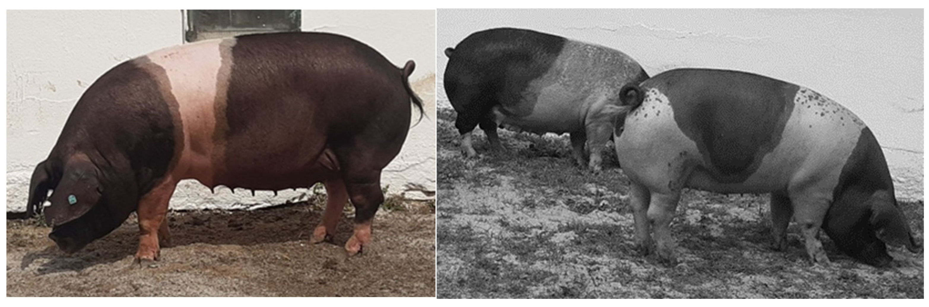
2.1. Animals
2.2. Pedigree Analysis
2.3. SNP Analysis
3. Results
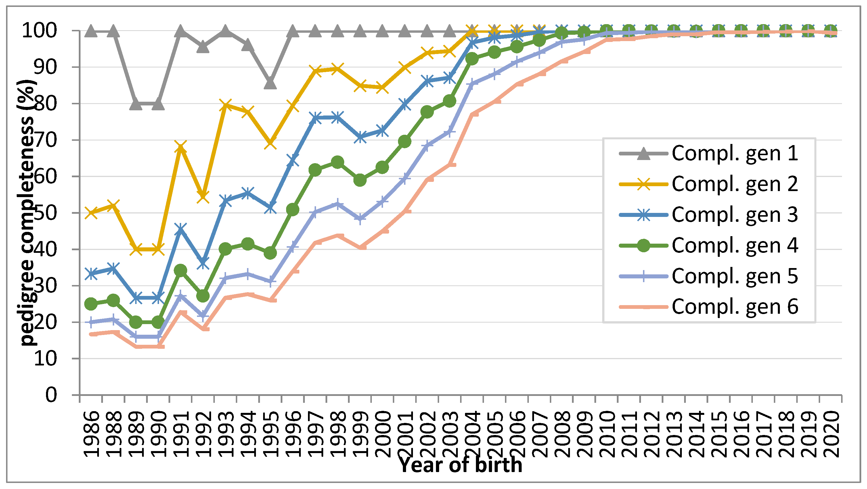
3.1. Quality of the Pedigree
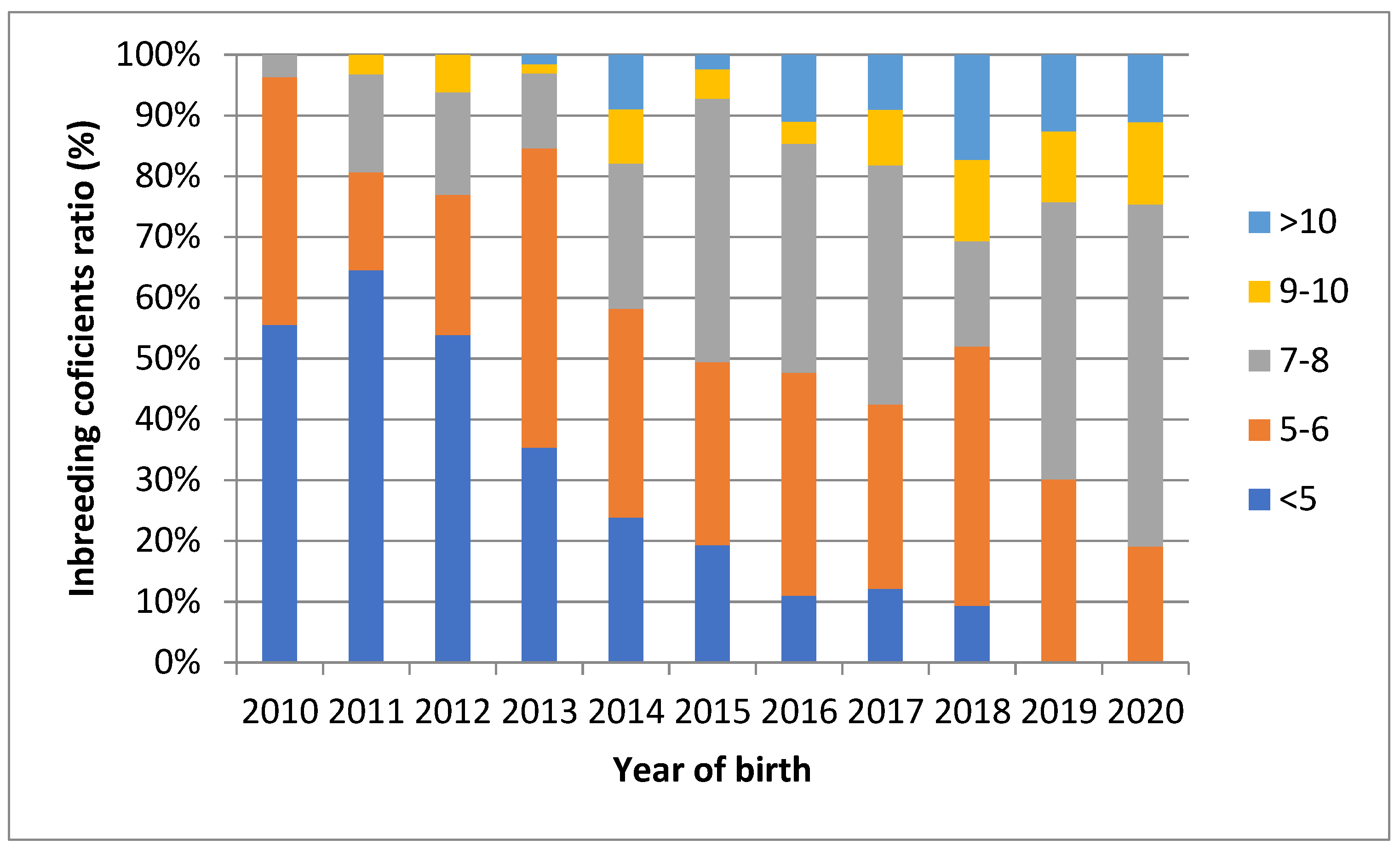
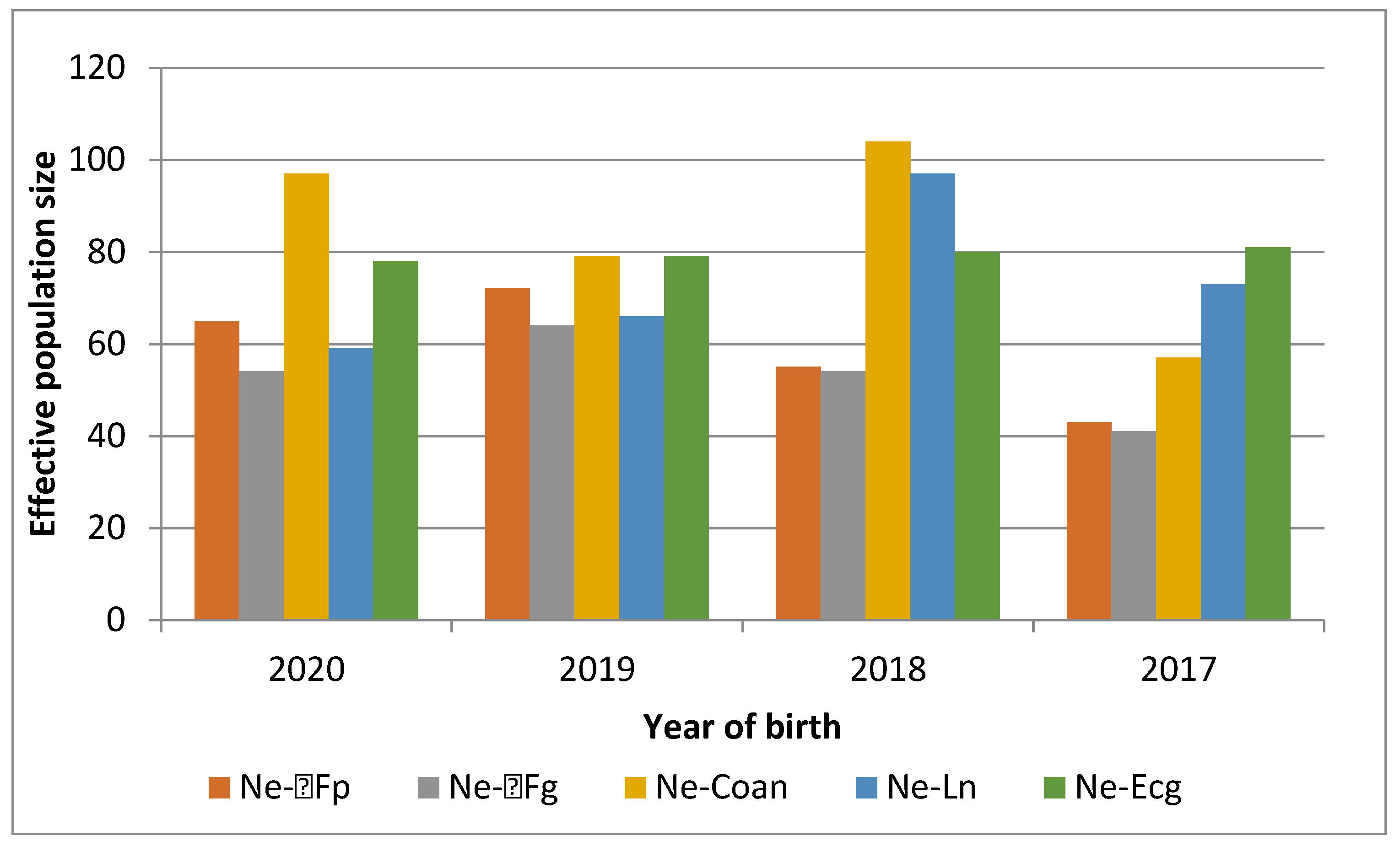
3.2. Analysis Based on the Pedigree Data
3.3. SNP Data Analysis
4. Discussion
4.1. Analysis Based on Pedigree Data
4.2. SNP Data Analysis
5. Conclusions
Supplementary Materials
Author Contributions
Funding
Institutional Review Board Statement
Informed Consent Statement
Data Availability Statement
Acknowledgments
Conflicts of Interest
References
- Fiedler, J.; Fiedlerová, M.; Smital, J. Přeštické Černostrakaté Plemeno Prasat, 1st ed.; VÚŽV: Praha, Czech Republic, 2004; p. 166. [Google Scholar]
- Hodan, J. Historie vzniku a průběh zvelebování chovu přeštického prasete. Pod Zelenou Horou Vlastivědný Sborník Jižního Plzeňska 1998, 1, 13. [Google Scholar]
- Vrtková, I. Genetic Admixture Analysis in Prestice Black-Pied Pigs. Arch. Anim. Breed. 2015, 58, 115–121. [Google Scholar] [CrossRef] [Green Version]
- Vaclavková, E.; Rozkot, M.; Dostálová, A. Přeštické Černostrakaté Prase. Živé Dědictví po Předcích (Přestice Black-Pied Pig—Living Heritage from Our Ancestors (Czech Language), 1st ed.; VÚŽV: Praha, Czech Republic, 2012; p. 70. [Google Scholar]
- Wolf, J.; Horáčková, Š.; Wolfová, M. Genetic Parameters for the Black Pied Přeštice Breed: Comparison of Different Multi-Trait Animal Models. Czech J. Anim. Sci. 2001, 46, 165–171. [Google Scholar]
- Matoušek, V.; Kernerová, N.; Hyšplerová, K.; Komosný, M. Performance Traits of Prestice Black-Pied Pig Breed at the Effect of Genealogical Line. Res. Pig Breed. 2016, 10, 10–15. [Google Scholar]
- FAO. The State of the World’s Biodiversity for Food and Agriculture; Food and Agriculture Organization: Rome, Italy, 2019; ISBN 9789251312704. [Google Scholar]
- Muñoz, M.; Bozzi, R.; García-Casco, J.; Núñez, Y.; Ribani, A.; Franci, O.; García, F.; Škrlep, M.; Schiavo, G.; Bovo, S.; et al. Genomic Diversity, Linkage Disequilibrium and Selection Signatures in European Local Pig Breeds Assessed with a High Density SNP Chip. Sci. Rep. 2019, 9, 13546. [Google Scholar] [CrossRef] [PubMed]
- Krupa, E.; Krupová, Z.; Žáková, E.; Kasarda, R.; Svitáková, A. Population Analysis of the Local Endangered Přeštice Black-Pied Pig Breed. Poljoprivreda 2015, 21, 155–158. [Google Scholar] [CrossRef]
- Wright, S. Coefficients of Inbreeding and Relationship. Am. Nat. 1922, 56, 330–338. [Google Scholar] [CrossRef] [Green Version]
- Meuwissen, T.H.E.; Luo, Z. Computing in Breeding Coefficients in Large Populations. Genet. Sel. Evol. 1992, 24, 305–313. [Google Scholar] [CrossRef]
- Falconer, D.S.; Mackay, T.F.C. Introduction to Quantitative Genetics, 4th ed.; Longman Scientific and Technical: Harlow, UK, 1996; p. 448. [Google Scholar]
- Colleau, J.J. An Indirect Approach to the Extensive Calculation of Relationship Coefficients. Genet. Sel. Evol. 2002, 34, 409–421. [Google Scholar] [CrossRef] [Green Version]
- Maccluer, J.W.; Boyce, A.J.; Dyke, B.; Weitkamp, L.R.; Pfenning, D.W.; Parsons, C.J. Inbreeding and Pedigree Structure in Standardbred Horses. J. Hered. 1983, 74, 394–399. [Google Scholar] [CrossRef]
- Sørensen, A.C.; Sørensen, M.K.; Berg, P. Inbreeding in Danish Dairy Cattle Breeds. J. Dairy Sci. 2005, 88, 1865–1872. [Google Scholar] [CrossRef] [Green Version]
- Krupa, E.; Žáková, E.; Krupová, Z. Evaluation of Inbreeding and Genetic Variability of Five Pig Breeds in Czech Republic. Asian-Australas. J. Anim. Sci. 2015, 28, 25–36. [Google Scholar] [CrossRef] [Green Version]
- Pérez-Enciso, M. Use of the Uncertain Relationship Matrix to Compute Effective Population Size. J. Anim. Breed. Genet. 1995, 112, 327–332. [Google Scholar] [CrossRef]
- Gutiérrez, J.P.; Cervantes, I.; Goyache, F. Improving the Estimation of Realized Effective Population Sizes in Farm Animals. J. Anim. Breed. Genet. 2009, 126, 327–332. [Google Scholar] [CrossRef]
- R Core Team. R: A Language and Environment for Statistical Computing; R Foundation for Statistical Computing: Vienna, Austria, 2020; Available online: https://www.R-project.org (accessed on 5 October 2021).
- Groeneveld, E.; Van der Westhuizen, B.; Maiwashe, A.; Voordewind, F.; Ferraz, J.B.S. POPREP: A Generic Report for Population Management. Genet. Mol. Res. 2009, 8, 1158–1178. [Google Scholar] [CrossRef]
- Sargolzaei, M.; Iwaisaki, H.; Colleau, J.J. CFC: A Tool for Monitoring Genetic Diversity. In Proceedings of the 8th World Congress on Genetics Applied to Livestock Production (WCGALP), Belo Horizonte, Brazil, 13–18 August 2006; pp. 27–28. [Google Scholar]
- Boichard, D. PEDIG: A Fortran Package for Pedigree Analysis Suited for Large Populations. In Proceedings of the 7th World Congress on Genetics Applied to Livestock Production (WCGALP), Montpellier, France, 19–23 August 2002; INRA: Castanet-Tolosan, France, 2002; pp. 19–23. [Google Scholar]
- Gutiérrez, J.P.; Goyache, F. A Note on ENDOG: A Computer Program for Analysing Pedigree Information. J. Anim. Breed. Genet. 2005, 122, 172–176. [Google Scholar] [CrossRef] [PubMed] [Green Version]
- Chang, C.C.; Chow, C.C.; Tellier, L.C.A.M.; Vattikuti, S.; Purcell, S.M.; Lee, J.J. Second-Generation PLINK: Rising to the Challenge of Larger and Richer Datasets. GigaScience 2015, 4, 7. [Google Scholar] [CrossRef]
- Lencz, T.; Lambert, C.; DeRosse, P.; Burdick, K.E.; Morgan, T.V.; Kane, J.M.; Kucherlapati, R.; Malhotra, A.K. Runs of Homozygosity Reveal Highly Penetrant Recessive Loci in Schizophrenia. Proc. Natl. Acad. Sci. USA 2007, 104, 19942–19947. [Google Scholar] [CrossRef] [Green Version]
- Marras, G.; Gaspa, G.; Sorbolini, S.; Dimauro, C.; Ajmone-Marsan, P.; Valentini, A.; Williams, J.L.; Macciotta, N.P. Analysis of Runs of Homozygosity and Their Relationship with Inbreeding in Five Cattle Breeds Farmed in Italy. Anim. Genet. 2015, 46, 110–121. [Google Scholar] [CrossRef] [PubMed]
- Ferenčakovič, M.; Hamzíc, E.; Gredler, B.; Solberg, T.R.; Klemetsdal, G.; Curik, I.; Sölkner, J. Estimates of Autozygosity Derived from Runs of Homozygosity: Empirical Evidence from Selected Cattle Populations. J. Anim. Breed. Genet. 2013, 130, 286–293. [Google Scholar] [CrossRef]
- Ferenčakovič, M.; Sölkner, J.; Curik, I. Estimating Autozygosity from High-Throughput Information: Effects of SNP Density and Genotyping Errors. Genet. Sel. Evol. 2013, 45, 42. [Google Scholar] [CrossRef] [Green Version]
- Schiavo, G.; Bovo, S.; Bertolini, F.; Tinarelli, S.; Dall’Olio, S.; Nanni Costa, L.; Gallo, M.; Fontanesi, L. Comparative Evaluation of Genomic Inbreeding Parameters in Seven Commercial and Autochthonous Pig Breeds. Animal 2020, 14, 910–920. [Google Scholar] [CrossRef] [PubMed]
- Santiago, E.; Novo, I.; Pardiñas, A.F.; Saura, M.; Wang, J.; Caballero, A. Recent Demographic History Inferred by High-Resolution Analysis of Linkage Disequilibrium. Mol. Biol. Evol. 2020, 37, 3642–3653. [Google Scholar] [CrossRef]
- Mitchell, M. An Introduction to Genetic Algorithms; MIT Press: Cambridge, UK, 1998. [Google Scholar]
- Pembleton, L.W.; Cogan, N.O.I.; Forster, J.W. StAMPP: An R Package for Calculation of Genetic Differentiation and Structure of Mixed-Ploidy Level Populations. Mol. Ecol. Resour. 2013, 13, 946–952. [Google Scholar] [CrossRef] [PubMed]
- Melka, M.G.; Schenkel, F. Analysis of Genetic Diversity in Four Canadian Swine Breeds Using Pedigree Data. Can. J. Anim. Sci. 2010, 90, 331–340. [Google Scholar] [CrossRef] [Green Version]
- Tang, G.Q.; Xue, J.; Lian, M.J.; Yang, R.F.; Liu, T.F.; Zeng, Z.Y.; Jiang, A.A.; Jiang, Y.Z.; Zhu, L.; Bai, L.; et al. Inbreeding and Genetic Diversity in Three Imported Swine Breeds in china Using Pedigree Data. Asian-Australas. J. Anim. Sci. 2013, 26, 755–765. [Google Scholar] [CrossRef] [Green Version]
- Veroneze, R.; Lopes, P.S.; Guimarães, S.E.F.; Guimarães, J.D.; Costa, E.V.; Faria, V.R.; Costa, K.A. Using Pedigree Analysis to Monitor the Local Piau Pig Breed Conservation Program. Arch. Zootec. 2014, 63, 45–54. [Google Scholar] [CrossRef] [Green Version]
- Mariani, E.; Summer, A.; Ablondi, M.; Sabbioni, A. Genetic Variability and Management in Nero di Parma Swine Breed to Preserve Local Diversity. Animals 2020, 10, 538. [Google Scholar] [CrossRef] [Green Version]
- Saura, M.; Fernández, A.; Varona, L.; Fernández, A.I.; de Cara, M.Á.; Barragán, C.; Villanueva, B. Detecting Inbreeding Depression for Reproductive Traits in Iberian Pigs Using Genome-Wide Data. Genet. Sel. Evol. 2015, 47, 1. [Google Scholar] [CrossRef] [PubMed] [Green Version]
- Toro, M.A.; Rodrigañez, J.; Silio, L.; Rodriguez, C. Genealogical Analysis of a Closed Herd of Black Hairless Iberian Pigs. Conserv. Biol. 2008, 14, 1843–1851. [Google Scholar] [CrossRef]
- Köck, A.; Fürst-Waltl, B.; Baumung, R. Effects of Inbreeding on Number of Piglets Born Total, Born Alive and Weaned in Austrian Large White and Landrace Pigs. Arch. Anim. Breed. 2009, 52, 51–64. [Google Scholar] [CrossRef] [Green Version]
- Silió, L.; Rodríguez, M.C.; Fernández, A.; Barragán, C.; Benítez, R.; Óvilo, C.; Fernández, A.I. Measuring Inbreeding and Inbreeding Depression on Pig Growth from Pedigree or SNP-Derived Metrics. J. Anim. Breed. Genet. 2013, 130, 349–360. [Google Scholar] [CrossRef] [PubMed]
- Welsh, C.S.; Stewart, T.S.; Schwab, C.; Blackburn, H.D. Pedigree Analysis of 5 Swine Breeds in the United States and the Implications for Genetic Conservation. J. Anim. Sci. 2010, 88, 1610–1618. [Google Scholar] [CrossRef] [PubMed] [Green Version]
- Meuwissen, T.H.E.; Woolliams, J.A. Effective Sizes of Livestock Populations to Prevent a Decline in Fitness. Theor. Appl. Genet. 1994, 89, 1019–1026. [Google Scholar] [CrossRef]
- Herrero-Medrano, J.M.; Megens, H.J.; Groenen, M.A.; Ramis, G.; Bosse, M.; Pérez-Enciso, M.; Crooijmans, R.P.M.A. Conservation Genomic Analysis of Domestic and Wild Pig Populations from the Iberian Peninsula. BMC Genet. 2013, 14, 106. [Google Scholar] [CrossRef] [PubMed] [Green Version]
- Hlongwane, N.L.; Hadebe, K.; Soma, P.; Dzomba, E.F.; Muchadeyi, F.C. Genome Wide Assessment of Genetic Variation and Population Distinctiveness of the Pig Family in South Africa. Front. Genet. 2020, 11, 344. [Google Scholar] [CrossRef] [PubMed]
- Laval, G.; Iannuccelli, N.; Legault, C.; Milan, D.; Groenen, M.A.; Giuffra, E.; Andersson, L.; Nissen, P.H.; Jørgensen, C.B.; Beeckmann, P.; et al. Genetic Diversity of Eleven European Pig Breeds. Genet. Sel. Evol. 2000, 32, 187–203. [Google Scholar] [CrossRef] [PubMed] [Green Version]
- Blackburn, H.; Faria, D.A.; Wilson, C.; Paiva, S.R. P4066 Genetic Diversity of Pig Populations from the US Mainland, Pacific Islands and China: Autosomal SNP Evaluation. J. Anim. Sci. 2016, 94, 112. [Google Scholar] [CrossRef]
- Zanella, R.; Peixoto, J.O.; Cardoso, F.F.; Cardoso, L.L.; Biegelmeyer, P.; Cantão, M.E.; Otaviano, A.; Freitas, M.S.; Caetano, A.R.; Ledur, M.C. Genetic Diversity Analysis of Two Commercial Breeds of Pigs Using Genomic and Pedigree Data. Genet. Sel. Evol. 2016, 48, 24. [Google Scholar] [CrossRef] [Green Version]
- Daetwyler, H.D.; Villanueva, B.; Bijma, P.; Woolliams, J.A. Inbreeding in Genome-wide Selection. J. Anim. Breed. Genet. 2007, 124, 369–376. [Google Scholar] [CrossRef]


| Parameter (Unit) | Sire | Dam | Total |
|---|---|---|---|
| Total number of animals in pedigree | 507 | 1466 | 1971 |
| Reference population in pedigree | 47 | 277 | 324 |
| Number of evaluated herds | 12 | 11 | 12 |
| Average number of: dams in a herd | 15.3 | ||
| Sires in a herd | 2.71 | ||
| Number of offspring selected per dam | 1.71 | ||
| Number of offspring selected per sire | 4.50 | ||
| Number of sires per dam | 1.19 | ||
| Number of dams per sire | 3.02 | ||
| Year of Evaluation | Generation Interval (in Years) in Different Paths 1 | ||||
|---|---|---|---|---|---|
| SS | SD | DS | DD | Population | |
| 2005 | 3.6 | 2.4 | 2.3 | 2.4 | 2.6 |
| 2010 | 1.8 | 2.0 | 2.3 | 2.4 | 2.1 |
| 2015 | 2.3 | 2.3 | 1.8 | 2.1 | 2.2 |
| 2020 | 3.3 | 2.8 | 2.2 | 2.2 | 2.6 |
| Mean | 3.0 | 2.5 | 2.6 | 2.2 | 2.5 |
| Year | Animals | Sires | Dams | |||
|---|---|---|---|---|---|---|
| n 1 in Total | F 2 | n in Total | F | n in Total | F | |
| 2018 | 75 | 7.49% | 26 | 7.03% | 54 | 6.82% |
| 2019 | 103 | 8.11% | 24 | 7.37% | 73 | 7.21% |
| 2020 | 126 | 8.10% | 32 | 6.67% | 82 | 7.43% |
| FAnN | FAnO | FAnT | FSrN | FSrO | FSrT | FDmN | FDmO | FDmT | |
|---|---|---|---|---|---|---|---|---|---|
| Avg. | 2.31 | 5.64 | 7.95 | 2.15 | 5.49 | 7.64 | 2.32 | 5.65 | 7.97 |
| s.d. | 2.51 | 0.71 | 2.61 | 1.54 | 0.71 | 1.79 | 1.6 | 2.61 | 1.83 |
| Min. | 0.00 | 2.87 | 4.31 | 0.00 | 2.87 | 5.05 | 0.00 | 3.14 | 4.31 |
| Max | 9.38 | 7.86 | 14.46 | 5.47 | 7.26 | 12.11 | 9.38 | 7.86 | 14.46 |
| ROH Class | No. of ROH | FROH (%) | ||||
|---|---|---|---|---|---|---|
| ± SD | Min | Max | ± SD | Min | Max | |
| 1 Mb | 41.931 ± 8.974 | 21 | 71 | 10.810 ± 3.634 | 3.225 | 23.663 |
| 2 Mb | 38.477 ± 8.725 | 19 | 68 | 10.571 ± 3.637 | 3.097 | 23.289 |
| 4 Mb | 21.190 ± 5.834 | 8 | 36 | 9.308 ± 3.578 | 2.438 | 23.486 |
| 8 Mb | 9.500 ± 3.941 | 1 | 21 | 6.722 ± 3.320 | 0.333 | 20.430 |
| 16 Mb | 3.517 ± 2.190 | 0 | 10 | 3.984 ± 2.758 | 0 | 14.801 |
| FROH1 | FROH2 | FROH4 | FROH8 | FROH16 | Fhat1 | Fhat2 | Fhat3 | |
|---|---|---|---|---|---|---|---|---|
| FPED | 0.519 | 0.513 | 0.510 | 0.542 | 0.491 | −0.026 | 0.508 | 0.307 |
| FROH1 | 0.998 | 0.967 | 0.895 | 0.795 | 0.222 | 0.844 | 0.659 | |
| FROH2 | 0.964 | 0.889 | 0.797 | 0.220 | 0.838 | 0.651 | ||
| FROH4 | 0.942 | 0.834 | 0.262 | 0.830 | 0.689 | |||
| FROH8 | 0.893 | 0.288 | 0.785 | 0.686 | ||||
| FROH16 | 0.237 | 0.716 | 0.585 | |||||
| Fhat1 | 0.032 | 0.771 | ||||||
| Fhat2 | 0.606 |
Publisher’s Note: MDPI stays neutral with regard to jurisdictional claims in published maps and institutional affiliations. |
© 2021 by the authors. Licensee MDPI, Basel, Switzerland. This article is an open access article distributed under the terms and conditions of the Creative Commons Attribution (CC BY) license (https://creativecommons.org/licenses/by/4.0/).
Share and Cite
Krupa, E.; Moravčíková, N.; Krupová, Z.; Žáková, E. Assessment of the Genetic Diversity of a Local Pig Breed Using Pedigree and SNP Data. Genes 2021, 12, 1972. https://doi.org/10.3390/genes12121972
Krupa E, Moravčíková N, Krupová Z, Žáková E. Assessment of the Genetic Diversity of a Local Pig Breed Using Pedigree and SNP Data. Genes. 2021; 12(12):1972. https://doi.org/10.3390/genes12121972
Chicago/Turabian StyleKrupa, Emil, Nina Moravčíková, Zuzana Krupová, and Eliška Žáková. 2021. "Assessment of the Genetic Diversity of a Local Pig Breed Using Pedigree and SNP Data" Genes 12, no. 12: 1972. https://doi.org/10.3390/genes12121972
APA StyleKrupa, E., Moravčíková, N., Krupová, Z., & Žáková, E. (2021). Assessment of the Genetic Diversity of a Local Pig Breed Using Pedigree and SNP Data. Genes, 12(12), 1972. https://doi.org/10.3390/genes12121972