Improving Modeling of Quinoa Growth under Saline Conditions Using the Enhanced Agricultural Policy Environmental eXtender Model


Abstract
:1. Introduction
2. Materials and Methods
2.1. Model Description
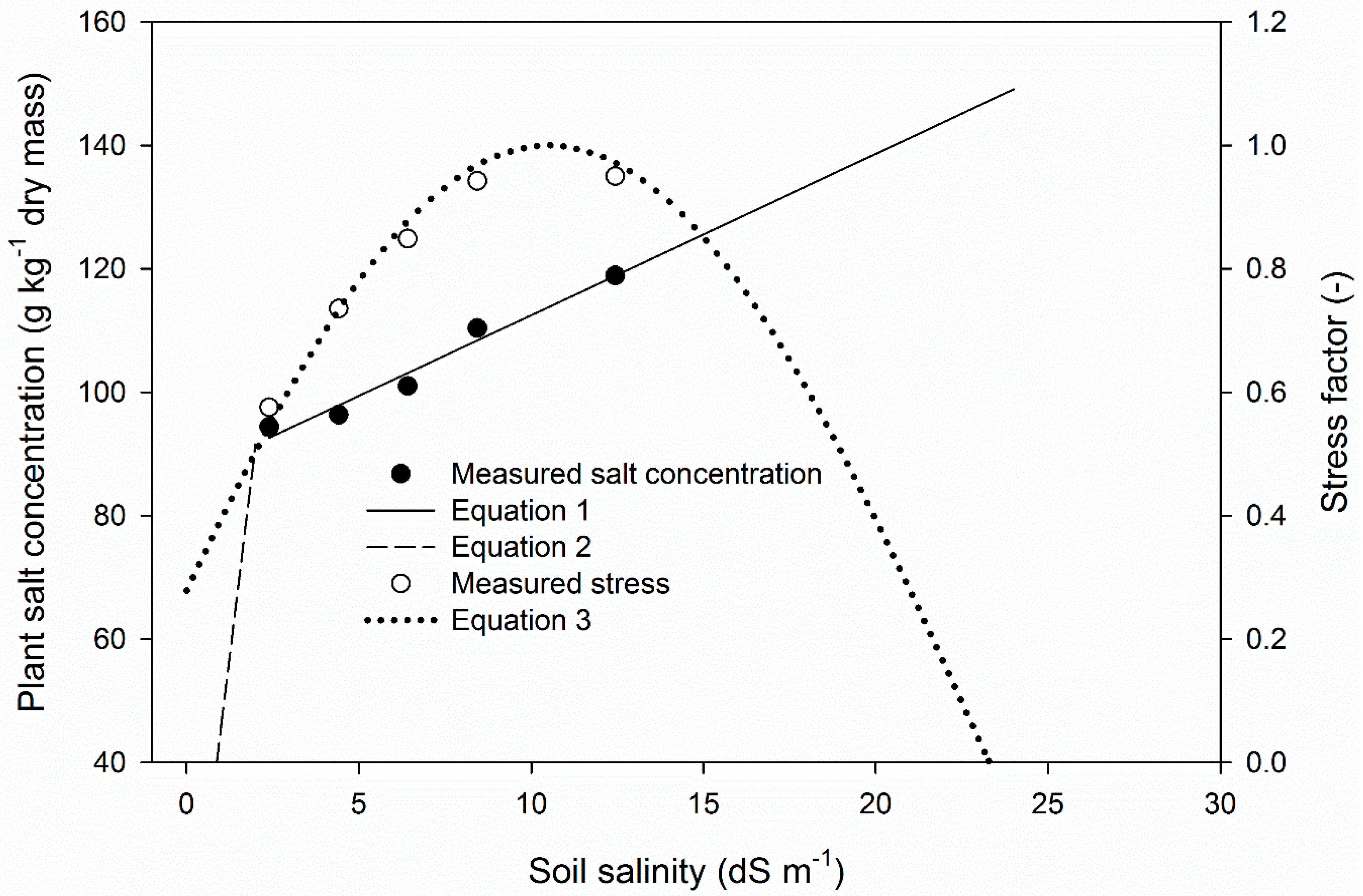
2.1.1. Plant Salt Uptake
2.1.2. Salt Stress
2.2. APEX Model Setup
2.2.1. Quinoa Parameterization
2.2.2. Soil Parameterization
2.2.3. Weather Inputs
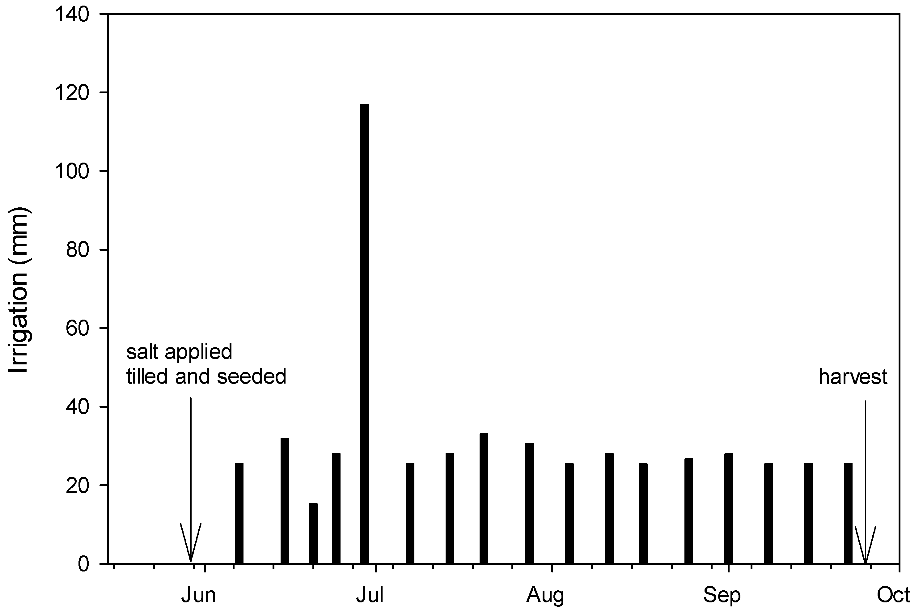
2.2.4. Management Inputs
2.3. Model Calibration
2.4. Long-Term Scenarios
3. Results
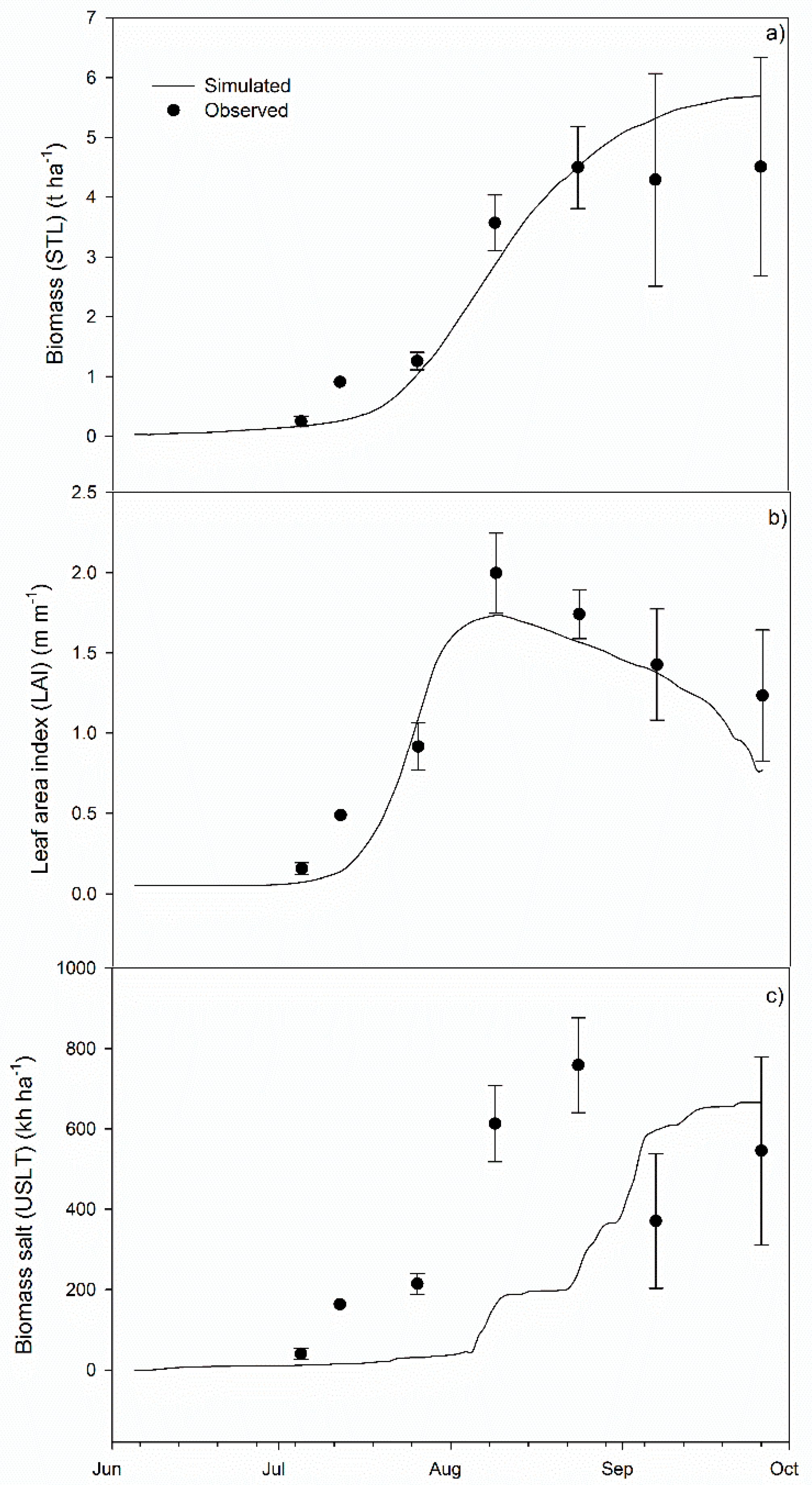
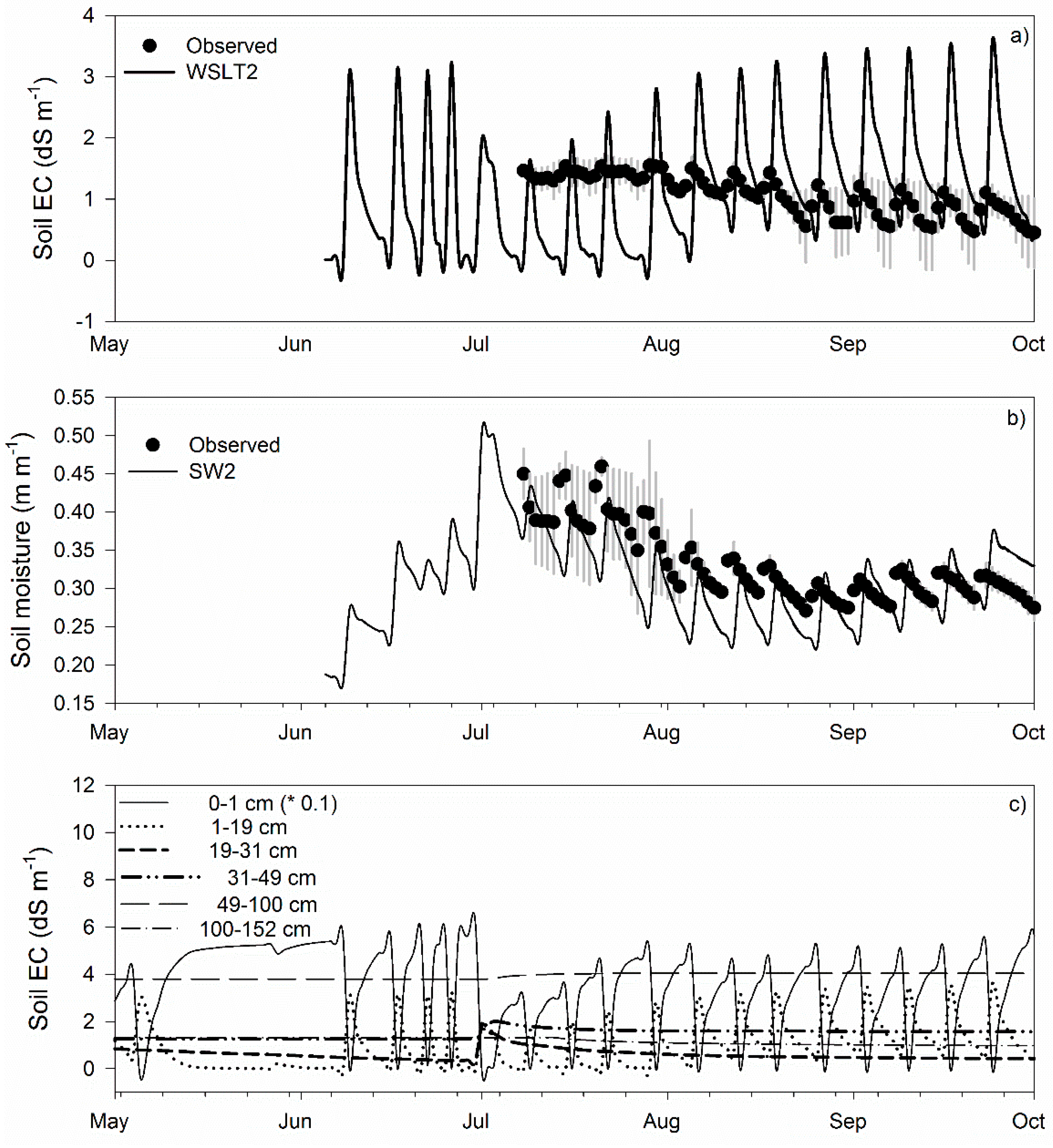
3.1. Calibration
3.2. 5-Year Scenarios
4. Discussion
5. Conclusions
Supplementary Materials
Author Contributions
Funding
Acknowledgments
Conflicts of Interest
Appendix A. Greenhouse Experiment
Appendix B. Field Experiment
Appendix C. Sensitivity Analysis
Sensitivity Analysis Results
References
- Munns, R. Genes and salt tolerance: Bringing them together. New Phytol. 2005, 167, 645–663. [Google Scholar] [CrossRef] [PubMed]
- Munns, R.; Tester, M. Mechanisms of salinity tolerance. Annu. Rev. Plant Biol. 2008, 59, 651–681. [Google Scholar] [CrossRef] [PubMed]
- Maas, E.V.; Hoffman, G.J. Crop salt tolerance—Current assessment. J. Irrig. Drain. Div. Am. Soc. Civ. Eng. 1977, 103, 115–134. [Google Scholar]
- Richards, L.A. Diagnosis and Improvement of Saline and Alkali Soils; Agriculture Handbook No. 60; US Department of Agriculture: Washington, DC, USA, 1954.
- Panta, S.; Flowers, T.; Lane, P.; Doyle, R.; Haros, G.; Shabala, S. Halophyte agriculture: Success stories. Environ. Exp. Bot. 2014, 107, 71–83. [Google Scholar] [CrossRef]
- Shabala, S.; Mackay, A. Ion transport in halophytes. Adv. Bot. Res. 2011, 57, 152–199. [Google Scholar]
- Flowers, T.J.; Colmer, T.D. Salinity tolerance in halophytes. New Phytol. 2008, 179, 945–963. [Google Scholar] [CrossRef] [PubMed]
- Akinshina, N.; Toderich, K.; Azizov, A.; Saito, L.; Ismail, S. Halophyte biomass—A promising source of renewable energy. J. Arid Land Stud. 2014, 24, 231–235. [Google Scholar]
- Adolf, V.I.; Shabala, S.; Anderson, M.; Razzaghi, F.; Jacobsen, S. Varietal differences of quinoa’s tolerance to saline conditions. Plant Soil 2012, 357, 117–129. [Google Scholar] [CrossRef]
- Ruiz, K.B.; Biondi, S.; Martinez, E.A.; Orsini, F.; Antognoni, F.; Jacobsen, S.E. Quinoa—A model crop for understanding salt-tolerance mechanisms in halophytes. Plant Biosyst. 2016, 150, 357–371. [Google Scholar] [CrossRef]
- Choukr-Allah, R.; Rao, N.; Hirich, A.; Shahid, M.; Alshankti, A.; Toderich, K.; Gill, S.; Butt, U.R. Quinoa for marginal environments: Toward future food and nutritional security in MENA and Central Asia Regions. Front. Plant Sci. 2016, 7, 346. [Google Scholar] [CrossRef]
- Adolf, V.I.; Jacobsen, S.; Shabala, S. Salt tolerance mechanisms in quinoa (Chenopodium quinoa Willd.). Environ. Exp. Bot. 2013, 92, 43–54. [Google Scholar] [CrossRef]
- Ventura, Y.; Eshel, A.; Pasternak, D.; Sagi, M. The development of halophyte-based agriculture: Past and present. Ann. Bot. 2015, 115, 529–540. [Google Scholar] [CrossRef] [PubMed]
- Kaya, C.I.; Yazar, A.; Sezen, S.M. SALTMED model performance on simulation of soil moisture and crop yield for quinoa irrigated using different irrigation systems, irrigation strategies and water qualities in Turkey. Agric. Agric. Procedia 2015, 4, 108–118. [Google Scholar] [CrossRef]
- Vermue, E.; Metselaar, K.; van der Zee, S.E.A.T.M. Modelling of soil salinity and halophyte crop production. Environ. Exp. Bot. 2013, 92, 186–196. [Google Scholar] [CrossRef]
- Ben Asher, J.; Beltrao, J.; Aksoy, U.; Anac, D.; Anac, S. Modeling the effect of salt removing species in crop rotation. Int. J. Energy Environ. 2012, 6, 350–359. [Google Scholar]
- Dominguez, A.; Tarjuelo, J.M.; de Juan, J.A.; Lopez-Mata, E.; Karam, F. Deficit irrigation under water stress and salinity conditions: The MOPECO-Salt Model. Agric. Water Manag. 2011, 98, 1451–1461. [Google Scholar] [CrossRef]
- Ragab, R. Integrated management tool for water, crop, soil and N-fertilizers: The SALTMED model. Irrig. Drain. 2015, 64, 1–12. [Google Scholar] [CrossRef]
- Kroes, J.G.; Wessleing, J.G.; van Dam, J.C. Integrated modelling of the soil-water-atmosphere-plant system using the model SWAP 2.0 an overview of theory and an application. Hydrol. Process. 2000, 14, 1993–2002. [Google Scholar] [CrossRef]
- van Dam, J.C.; Groenendijk, P.; Hendriks, R.F.A.; Krose, J.G. Advances of modeling water flow in variably saturated soils with SWAP. Vadose Zone J. 2008, 7, 640–653. [Google Scholar] [CrossRef]
- Letey, J.; Vaughan, P. ENVIRO-GRO User Manual; University of California, Division of Agriculture and Natural Resources, California Institute for Water Resources: Oakland, CA, USA, 2013. [Google Scholar]
- Oster, J.D.; Letey, J.; Vaughan, P.; Wu, L.; Qadir, M. Comparison of transient state models that include salinity and matric stress effects on plant yield. Agric. Manag. Water Qual. 2012, 103, 167–175. [Google Scholar] [CrossRef]
- Williams, J.R.; Izaurralde, R.C.; Steglich, E.M. Agricultural Policy/Environmental Extender Model Theoretical Documentation; Version 0806; Blackland Research and Extension Center: Temple, TX, USA, 2012. [Google Scholar]
- Gassman, P.W.; Williams, J.R.; Wang, X.; Salch, A.; Osei, E.; Hauck, L.M.; Izaurralde, R.C.; Flowers, J.D. The Agricultural Policy/Environmental Extender (APEX) model: An emerging tool for landscape and watershed environmental analysis. Trans. ASABE 2010, 53, 711–740. [Google Scholar] [CrossRef]
- Steglich, E.M.; Williams, J.W. Agricultural Policy/Environmental Extender Model User’s Manual; Version 0806; BREC Report # 2008-16; Blackland Research and Extension Center: Temple, TX, USA, 2008; Available online: https://blackland.tamu.edu/files/2012/10/APEX.manual.pdf (accessed on 26 May 2019).
- Rhoades, J.D.; Manteghi, N.A.; Shouse, P.J.; Alves, W.J. Estimating soil salinity from saturated soil-paste electrical conductivity. Soil Sci. Soc. Am. J. 1989, 53, 428–433. [Google Scholar] [CrossRef]
- Kiniry, J.; USDA ARS, Grassland Soil and Water Research Laboratory, Temple, TX, USA. Personal communication, 2017.
- DeRuyter, T. Modeling Halophytic Plants to Improve Agricultural Production and Water Quality in Arid and Semi-Arid Regions. Master’s Thesis, University of Nevada, Reno, Reno, NV, USA, 2014. [Google Scholar]
- Grattan, S.R.; Oster, J.D.; Benes, S.E.; Kaffka, S.R. Use of saline drainage waters for irrigation. In Agricultural Salinity Assessment and Management, 2nd ed.; Wallender, W.W., Tanji, K.K., Eds.; American Society of Civil Engineers: Reston, VA, USA, 2012; pp. 687–719. [Google Scholar]
- 1981–2010 Normals for Reno-Tahoe International Airport, NV US. National Centers for Environmental Information, National Oceanic and Atmospheric Administration. Available online: https://www.ncdc.noaa.gov/cdo-web/datatools/normals (accessed on 1 May 2017).
- Tanji, K.K. Salinity in the soil environment. In Salinity: Environment-Plants-Molecules; Lauchli, A., Luttge, U., Eds.; Kluwer Academic Publishers: Dordrecht, The Netherlands, 2002; pp. 21–51. [Google Scholar]
- Tester, M.; Davenport, R. Na+ tolerance and Na+ transport in higher plants. Ann. Bot. 2003, 91, 503–527. [Google Scholar] [CrossRef] [PubMed]
- Bonales-Alatorre, E.; Shabala, S.; Chen, Z.; Pottosin, I. Reduced tonoplast fast-activating and slow-activating channel activity is essential for conferring salinity tolerance in a facultative halophyte, quinoa. Plant Physiol. 2013, 162, 940–952. [Google Scholar] [CrossRef] [PubMed]
- Pulvento, C.; Riccardi, M.; Lavini, A.; D’Andria, R.; Ragab, R. SALTMED model to simulate yield and dry matter for quinoa crop and soil moisture content under different irrigation strategies in south Italy. Irrig. Drain. 2013, 62, 229–238. [Google Scholar] [CrossRef]
- Kaya, C.I.; Yazar, A. SALTMED model performance for quinoa irrigated with fresh and saline water in a Mediterranean environment. Irrig. Drain. 2016, 65, 29–37. [Google Scholar] [CrossRef]
- Rabhi, M.; Hafsi, C.; Lakhdar, A.; Hajji, S.; Barhoumi, Z.; Hamrouni, M.; Abdelly, C.; Smaoui, A. Evaluation of the capacity of three halophytes to desalinize their rhizosphere as grown on saline soils under nonleaching conditions. Afr. J. Ecol. 2009, 47, 463–468. [Google Scholar] [CrossRef]
- Goehring, N. Modeling Salt Movement and Halophytic Crop Growth on Marginal Lands with the APEX Model. Master’s Thesis, University of Nevada, Reno, Reno, NV, USA, 2017. [Google Scholar]
- Lutsch, B.; City of Sparks, Sparks, NV, USA. Personal communication, 2016.
- Kiniry, J.; USDA ARS, Grassland Soil and Water Research Laboratory, Temple, TX, USA. Personal communication, 2016.

| Scenario Code | Annual Irrigation (mm) | Irrigation Salinity (ppm) |
|---|---|---|
| LO-NS | 272 | 420 |
| MID-NS | 544 | 420 |
| HI-NS | 970 | 420 |
| LO-S | 272 | 3000 |
| MID-S | 544 | 3000 |
| HI-S | 970 | 3000 |
| Cal. Stage | Output Variable | Units | n | Observed Range | RMSE | R2 |
|---|---|---|---|---|---|---|
| 1 | STL | t/ha | 7 | 0.25–4.51 | 0.57 | 0.93 |
| 1 | LAI | 7 | 0.16–2.00 | 0.28 | 0.90 | |
| 1 | SW2 | m/m | 146 | 0.24–0.46 | 0.064 | 0.020 |
| 1 | USLT | kg/ha | 7 | 39.6–758.4 | 216.3 | 0.48 |
| 1 | WSLT2 | dS/m | 146 | 0.44–1.55 | 2.91 | 0.60 |
| 2 | STL | t/ha | 7 | 0.25–4.51 | 0.70 | 0.93 |
| 2 | LAI | 7 | 0.16–2.00 | 0.26 | 0.90 | |
| 2 | SW2 | m/m | 146 | 0.24–0.46 | 0.065 | 0.016 |
| 2 | USLT | kg/ha | 7 | 39.6–758.4 | 291.0 | 0.23 |
© 2019 by the authors. Licensee MDPI, Basel, Switzerland. This article is an open access article distributed under the terms and conditions of the Creative Commons Attribution (CC BY) license (http://creativecommons.org/licenses/by/4.0/).
Share and Cite
Goehring, N.; Verburg, P.; Saito, L.; Jeong, J.; Meki, M.N. Improving Modeling of Quinoa Growth under Saline Conditions Using the Enhanced Agricultural Policy Environmental eXtender Model. Agronomy 2019, 9, 592. https://doi.org/10.3390/agronomy9100592
Goehring N, Verburg P, Saito L, Jeong J, Meki MN. Improving Modeling of Quinoa Growth under Saline Conditions Using the Enhanced Agricultural Policy Environmental eXtender Model. Agronomy. 2019; 9(10):592. https://doi.org/10.3390/agronomy9100592
Chicago/Turabian StyleGoehring, Nicole, Paul Verburg, Laurel Saito, Jaehak Jeong, and Manyowa N. Meki. 2019. "Improving Modeling of Quinoa Growth under Saline Conditions Using the Enhanced Agricultural Policy Environmental eXtender Model" Agronomy 9, no. 10: 592. https://doi.org/10.3390/agronomy9100592
APA StyleGoehring, N., Verburg, P., Saito, L., Jeong, J., & Meki, M. N. (2019). Improving Modeling of Quinoa Growth under Saline Conditions Using the Enhanced Agricultural Policy Environmental eXtender Model. Agronomy, 9(10), 592. https://doi.org/10.3390/agronomy9100592