Process Importance Identification for the SPAC System Under Different Water Conditions: A Case Study of Winter Wheat

Abstract

Modeling the soil–plant–atmosphere continuum (SPAC) system requires multiple subprocesses and numerous parameters. Sensitivity analysis is effective to identify important model components and improve the modeling efficiency. However, most sensitivity analyses for SPAC models focus on parameter-level assessment, providing limited insights into process-level importance. To address this gap, this study proposes a process sensitivity analysis method that integrates the Bayesian network with variance-based sensitivity measures. Four subprocesses are demarcated based on the physical relationships between model components revealed by the network. Applied to a winter wheat SPAC system under different water conditions, the method effectively and reliably identifies critical processes. The results indicate that, under minimal water stress, the subprocesses of photosynthesis and dry matter partitioning primarily determine agricultural outputs. As the water supply decreases, the subprocesses of soil water movement and evapotranspiration gain increasing importance, becoming predominant under sever water stress. Throughout the crop season, the subprocess importance and its response to water stress are modulated by the crop phenology. Compared to conventional parameter sensitivity analysis, our method excels in synthesizing divergent parameter importance changes and identifying influential subprocesses, even without high-sensitivity parameters. This study provides new insights into adaptive SPAC modeling by dynamically simplifying unimportant subprocesses in response to environmental changes.

1. Introduction

The soil–plant–atmosphere continuum (SPAC) system serves as the theoretical foundation for agricultural modeling [1,2,3]. Over decades of development, the concept of SPAC has evolved to encompass various physical, physiological, and chemical processes governing the transport and transformation of matter (e.g., water, carbon) and energy (e.g., potential, light) [4]. To account for component diversity, physical heterogeneity, and environmental spatiotemporal variability, SPAC models have become increasingly complex and massive. However, this poses practical challenges, as the model configuration needs to be localized for specific scenarios, but determining every model component (e.g., parameter, equation) is impractical due to limited measurement and computational resources. Fortunately, such exhaustive model localization is often unnecessary, as only a small subset of model components significantly influence specific simulation outputs in a given scenario [5,6]. Therefore, a principled method to identify key model components is essential.

Sensitivity analysis has almost become a standard practice in identifying key model components in applications [7,8]. The basic idea is to quantify how much the uncertainty in the simulation output is induced by individual uncertain components. Components that cause large output uncertainty are identified as important and require careful determination. The total model uncertainty primarily stems from three sources: input uncertainty, parameter uncertainty, and structural uncertainty (e.g., equation formalization) [9]. In practice, when applying a SPAC model, the inputs of meteorological forcing and farmland management are usually known. The parameter and structural uncertainties are the major uncertainty sources in agricultural simulations. However, most works focus solely on parameter sensitivity analysis and ensure that the outputs match observations by merely adjusting the parameter values [10,11,12]. This may introduce errors, because parameter values are optimized within a predefined model structure, and potential structural bias will be compensated for by parameter adjustments [13,14]. Consequently, insights derived from varying parameter values across different scenarios may be misleading. This issue is noteworthy as research has revealed that, in agricultural simulations, the structural uncertainty can be larger than the parameter uncertainty [15,16]. Thus, to enhance the reliability of SPAC simulations, it is essential to develop a sensitivity analysis method that accounts for structural influences.

Existing studies on structural uncertainty quantification, which typically involve multiple alternative models [15,16], remain insufficient as they do not directly identify critical structural components within each candidate model. The SPAC system is inherently process-based, and SPAC models usually comprise several coupled yet relatively independent subprocesses, such as soil water movement and evapotranspiration. Understanding the influence of individual subprocesses and their interactions under varying environmental conditions is crucial in accurately characterizing system behavior [17,18]. These considerations underscore the significance of assessing structural importance at the process level.

Within a system model, the influence of a subprocess stems from both its associated parameters and the interactions among these parameters through process conceptualization and equations. Some studies suggest that the sensitivity of appropriately grouped parameters can serve as a proxy for the measurement of processes’ importance [19,20,21]. Variance-based methods [22] have made contributions to this, owing to their capacity to decompose the total variance of the model output into variance terms attributable to any possible parameter subsets. However, not all parameter subsets can represent processes; they must have relationships consistent with the process mechanism. Baroni and Tarantola [21] were among the first to develop a sensitivity analysis for physically correlated parameters, predefining mutually exclusive groups and using pre-sampled parameter sets. Mai et al. [19] advanced process sensitivity analysis by allowing each parameter to be flexibly assigned to multiple processes and offering a computationally efficient procedure for sensitivity calculation. However, in their sampling for process uncertainties, they neglected the fact that some processes depend on outputs from other specific processes. Hence, a process sensitivity analysis method that can reasonably define parameter groups while accounting for physical dependencies between processes remains lacking.

The Bayesian network (BN) [23] provides a potential solution to these challenges. On one hand, its directed acyclic graph can explicitly represent the physical dependencies among all model components, illustrating how parameter uncertainty propagates within and across processes to influence the output. On the other hand, its statistical framework, based on conditional probability and probability factorization, possess good compatibility with the already established variance-based method. Dai et al. [24] incorporated the BN into the sensitivity analysis of a groundwater biogeochemical reactive transport model and demonstrated its effectiveness in representing various uncertain model components with hierarchical relationships. While their study considered process sensitivity, it did not fully account for process uncertainty arising from interactions between uncertain parameters. Moreover, the sensitivity metrics that they derived were specific to the BN structure, which itself depends on the employed model. Thus, integrating the BN into process sensitivity analysis for SPAC system models remains a challenge.

To address this, this study aims to establish a new sensitivity method that combines parameter grouping and the BN. In this way, we aim to identify important process while respecting their physical relationships within the SPAC system. The new method is demonstrated and evaluated through a real-world application to simulate winter wheat growth under different water conditions using the soil–water–atmosphere–plant (SWAP) model [25]. By comparing our method to conventional parameter sensitivity analysis, we consider the differences that can be obtained by considering or neglecting mechanistic interactions between parameters. The sensitivity analysis is conducted for multiple model outputs across different crop growth stages. Beyond providing a practical tool for the identification of structural components that may need refinement or simplification, this study aims to shed scientific light on the following questions: (1) Which subprocesses contribute the most to crop growth, yields, and water use efficiency? (2) How do subprocesses’ contributions vary under different water stress levels? (3) How do subprocesses’ contributions change over time across different crop growth stages?

2. Materials and Methods

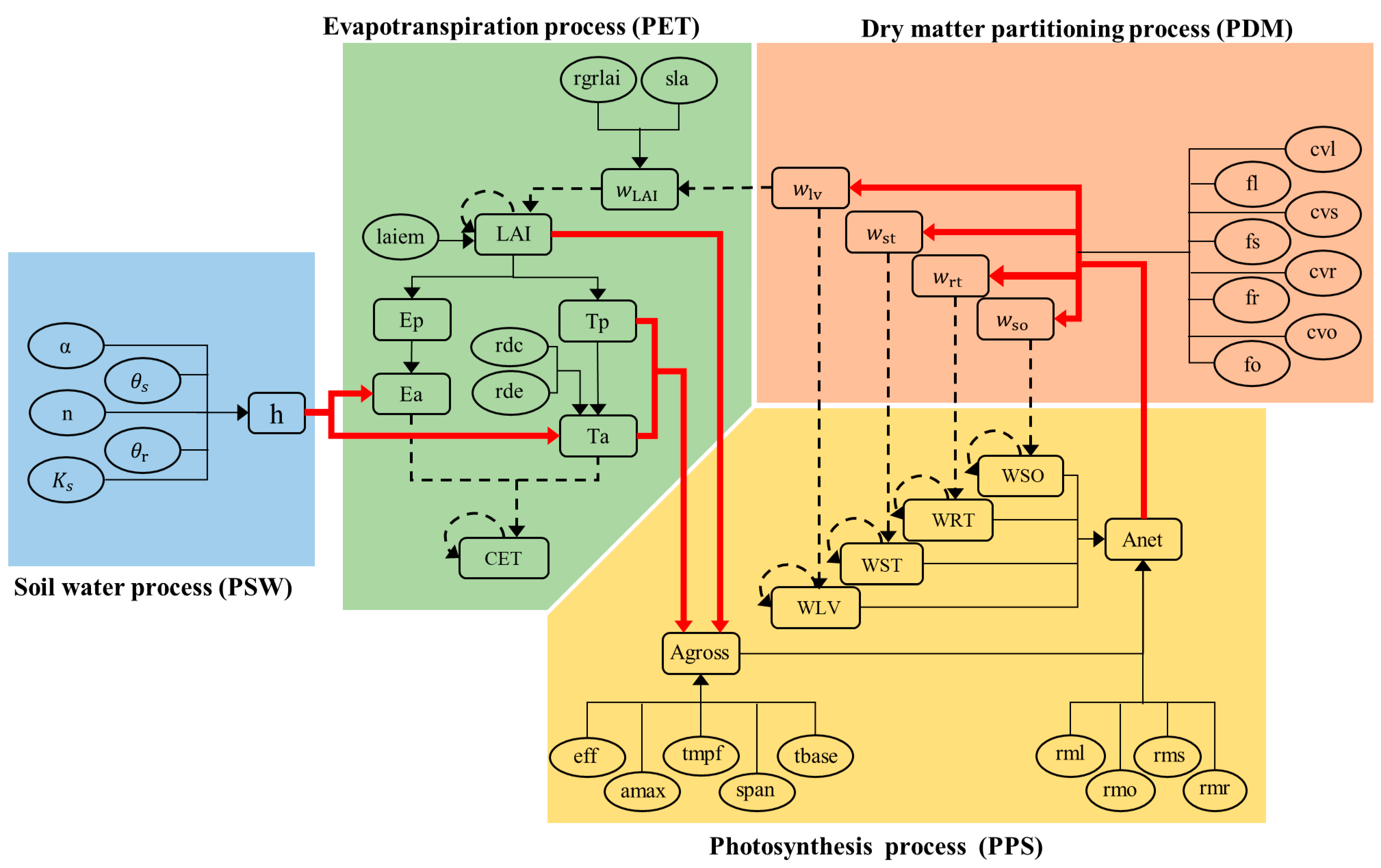
2.1. Description of the SWAP Model Simulation for the SPAC System

This study employs the SWAP model (version 3.2) [25] as a representative SPAC model. It simulates dynamic plant growth with detailed physiological activities, water transport in the vadose zone, and interactions between soil, plants, and the atmosphere. Widely used in agriculture and ecohydrology over the past few decades [26], SWAP effectively captures the complex mechanisms governing the SPAC system.

With proper initial soil moisture and crop states, SWAP runs simulations based on daily meteorological inputs and the irrigation regime (if applicable). Meteorological inputs include precipitation, radiation, the minimum and maximum temperatures, the air humidity, and the wind speed. While it can provide a wide range of SPAC-related outputs, this study focuses on five key agricultural variables: the leaf area index (LAI, m²/m²), the dry weight of the storage organs (e.g., wheat grains) (WSO, kg/ha), the total dry weight of all organs (TW, kg/ha), the water consumption coefficient of storage organs (SWCC, m³/kg), and the water consumption coefficient of the total dry weight (TWCC, m³/kg). These coefficients quantify the water use efficiency by calculating how much water is consumed per unit of dry weight:

$$\mathrm{S}\mathrm{W}\mathrm{C}\mathrm{C}={\displaystyle \frac{\mathrm{C}\mathrm{E}\mathrm{T}}{\mathrm{W}\mathrm{S}\mathrm{O}}},$$

(1)

$$\mathrm{T}\mathrm{W}\mathrm{C}\mathrm{C}={\displaystyle \frac{\mathrm{C}\mathrm{E}\mathrm{T}}{\mathrm{T}\mathrm{W}}},$$

(2)

where CET is the cumulative evapotranspiration (mm) from the beginning of the crop season.

The major processes governing the dynamics of these five variables in SWAP are as follows.

Soil water flow is simulated using Richards’ equation [27], with soil hydraulic properties defined by the Mualem–Van Genuchten relation [28]. Key parameters include the saturated hydraulic conductivity ($K_S$), saturated water content (${\theta }_S$), residual water content (${\theta }_r$), and two shape parameters of the soil water retention curve (α and n). Solving Richards’ equation yields the temporal evolution of the soil water content ($\theta$) and pressure head (h) across the soil profile. The water pressure head determines crop water availability by affecting the water potential gradient between the roots and soil.

Evapotranspiration defines the atmospheric water demand on the crop and, together with soil water availability, regulates crop water stress. Specifically, the daily potential evapotranspiration is calculated from meteorological inputs using the Penman–Monteith equation and then partitioned into the potential evaporation ($E_p$) and transpiration ($T_p$) based on the land cover fraction represented by the LAI. $E_p$ may decrease to the lower actual evaporation ($E_a$) depending on the wetness of the top soil. The reduction from $T_p$ to the lower actual transpiration ($T_a$) considers the water availability within the entire root zone and thus is influenced by the rooting depth (rdc) and root distribution density (rde). The $T_a/T_p$ ratio serves as an indicator of crop water stress.

Water stress reduces the gross CO₂ assimilation rate ($A_{gross}$) as a reduction factor below one. The CO₂ assimilation is influenced by many factors. Externally, only a fraction of the radiation fluxes can be captured, depending on the canopy density, which is characterized by the LAI. Internally, leaf-level photosynthesis is parameterized by the light use efficiency (eff), the maximum CO₂ assimilation rate at light saturation (amax), and its reduction factor due to suboptimal temperature (tmpf). At the canopy level, not all leaves participate in photosynthesis, which depends on the leaf age and is characterized by the parameters tbase and span. Some of the carbohydrates formed through CO₂ assimilation are respired to maintain the existing biostructures, dependent on the dry weights of the leaves (WLV), stems (WST), roots (WRT), and storage organs (WSO), along with their maintenance coefficients (rml, rms, rmr, rmo). The remaining assimilates form the net assimilation rate ($A_{net}$).

$A_{net}$ is the amount of carbohydrates available for structural organ growth. The dry weight increase of each organ ($w_{\mathrm{l}\mathrm{v}}$, $w_{\mathrm{s}\mathrm{t}}$, $w_{\mathrm{r}\mathrm{t}}$ and $w_{\mathrm{s}\mathrm{o}}$) results from the partitioning of $A_{net}$ among individual organs (specified by parameters fl, fs, fr, and fo) and their respective conversion efficiencies (cvl, cvs, cvr, and cvo). Organ dry weights accumulate over time, and a leaf dry weight increase contributes to LAI growth ($w_{\mathrm{L}\mathrm{A}\mathrm{I}}$), characterized by the parameters sla and rgrlai.

The descriptions of these parameters are presented in

Table 1. Descriptions of the parameters included in this study and their variation ranges.

Parameter	Description	Unit	Variation Range
${\theta }_r$	Residual water content	cm3/cm3	0.017–0.026
${\theta }_s$	Saturated water content	cm3/cm3	0.450–0.674
$\mathsf{\alpha }$	Shape parameter of main drying curve	1/cm	0.0393–0.0590
n	Shape parameter	-	1.219–1.828
$K_s$	Saturated vertical hydraulic conductivity	cm/d	17.03–25.55
laiem	Leaf area index at emergence	m2/m2	0.2918–0.4376
rgrlai	Maximum relative increase in LAI	m2/m2/d	0.00877–0.01316
sla0.88	Specific leaf area at Dvs = 0.88	ha/kg	0.00120–0.00180
rde0.33	Relative root density when relative rooting depth is 0.33	-	0.31469–0.47203
rde0.67	Relative root density when relative rooting depth is 0.67	-	0.05000–0.07500
rde1.00	Relative root density when relative rooting depth is 1.00	-	0.01248–0.01872
rdc	Maximum rooting depth of crop	cm	65.32–97.97
span	Life span of leaves under optimum conditions	d	27.29–40.93
tbase	Lower threshold temperature for aging of leaves	°C	1.45–2.17
eff	Light use efficiency of leaves	kg CO2/J	0.474–0.711
amax0	Max CO2 assimilation rate at Dvs = 0	kg/ha/h	32.000–48.000
amax1	Max CO2 assimilation rate at Dvs = 1	kg/ha/h	29.906–44.860
amax2	Max CO2 assimilation rate at Dvs = 2	kg/ha/h	16.000–24.000
tmpf0	Reduction factor of amax when average day temperature is 0 °C	-	0.008–0.012
tmpf10	Reduction factor of amax when average day temperature is 10 °C	-	0.493–0.740
tmpf30	Reduction factor of amax when average day temperature is 30 °C	-	0.400–0.600
rml	Relative maintenance respiration rate of leaves	kgCH2O/kg/d	0.01480–0.02220
rms	Relative maintenance respiration rate of storage organs	kgCH2O/kg/d	0.01564–0.02346
rmr	Relative maintenance respiration rate of roots	kgCH2O/kg/d	0.01200–0.01800
rmo	Relative maintenance respiration rate of stems	kgCH2O/kg/d	0.01879–0.02819
cvl	Efficiency of carbohydrate conversion into leaves	kg/kg	0.5601–0.8402
cvs	Efficiency of carbohydrate conversion into storage organs	kg/kg	0.5845–0.8768
cvr	Efficiency of carbohydrate conversion into roots	kg/kg	0.5552–0.8328
cvo	Efficiency of carbohydrate conversion into stems	kg/kg	0.5517–0.8275
fr0	Fraction of total dry matter increase partitioned to roots at Dvs = 0	kg/kg	0.320–0.480
fr0.4	Fraction of total dry matter increase partitioned to roots at Dvs = 0.4	kg/kg	0.120–0.180
fr0.9	Fraction of total dry matter increase partitioned to roots at Dvs = 0.9	kg/kg	0.008–0.012
fl0	Fraction of total dry matter increase partitioned to leaves at Dvs = 0	kg/kg	0.480–0.720
fl0.5	Fraction of total dry matter increase partitioned to leaves at Dvs = 0.5	kg/kg	0.5967–0.8951
fs0.95	Fraction of total dry matter increase partitioned to stems at Dvs = 0.95	kg/kg	0.7024–1.0000
fo1	Fraction of total dry matter increase partitioned to storage organs at Dvs = 1	kg/kg	0.6472–0.9708

.

2.2. Subprocess Sensitivity Analysis Based on BN

A BN is an acyclic directed graph with nodes representing the variables and directional edges describing the conditional dependence or kinship relationships among the nodes [23]. For example, a directional edge from node $X_1$ to node $X_2$ means a cause–effect or parent–child relation between them, i.e., $X_1$ is a cause (parent) of $X_2$, and $X_2$ is one effect (child) of $X_1$. In a BN containing N nodes, node $X_i \left(i=1,\dots ,N\right)$ can have multiple parent nodes, denoted as $\mathrm{p}\mathrm{a}\mathrm{r}\mathrm{e}\mathrm{n}\mathrm{t}\mathrm{s}\left(X_i\right)$. Its uncertainty is propagated from its parents via the conditional probability $p\left(X_i|\mathrm{p}\mathrm{a}\mathrm{r}\mathrm{e}\mathrm{n}\mathrm{t}\mathrm{s}\left(X_i\right)\right)$. For root nodes, i.e., nodes that have no parents, the conditional probability simplifies to a marginal probability, and the uncertainty originates from these nodes themselves. Another specific type of node is deterministic nodes, whose values are entirely determined when given the values of their parents, instead of being linked through conditional probabilities. Based on the conditional dependence or independence contained in the acyclic directed graph, the full joint distribution of the BN can be computed as the product of the conditional probabilities of all nodes given their parents:

$$p\left(X_1,\dots , X_N\right)=\prod _{i=1}^{N}p\left(X_i|\mathrm{p}\mathrm{a}\mathrm{r}\mathrm{e}\mathrm{n}\mathrm{t}\mathrm{s}\left(X_i\right)\right).$$

(3)

According to the description in Section 2.1, we constructed a BN for the SPAC system simulation, as shown in Figure 1. The parameters with uncertain values are root nodes. Once the parameter values are given, the values of intermediary variables (e.g., $A_{gross}$) and state variables (e.g., WLV) are determined through the process-based equations during the simulations. Thus, they are deterministic nodes in the BN. Consistent with the process-based feature of the SPAC system, the nodes in the BN tend to cluster into groups. Based on the structural aggregation and physical knowledge, we demarcate four subprocesses in this study, namely the soil water process (PSW), evapotranspiration process (PET), photosynthesis process (PPS), and dry matter partitioning process (PDM), which are represented by colored boxes in Figure 1. Their interconnections are highlighted with red bold links.

2.2.1. Variance Decomposition for Subprocesses

The variance-based sensitivity analysis assesses the sensitivity of one uncertain model component by its contribution to the total output variance. Regarding a specific component $u_i$, the total variance of a target output Y can be decomposed as [29]

$$V\left(Y\right)=V_{u_i}\left(E_{{\mathit{U}}_{~\mathit{i}}}\left(Y|u_i\right)\right)+E_{u_i}\left(V_{{\mathit{U}}_{~\mathit{i}}}\left(Y|u_i\right)\right).$$

(4)

where $V$ and $E$ are the notations for variance and expectation calculations, respectively, and ${\mathit{U}}_{~\mathit{i}}$ denotes all other components except $u_i$. The first term on the right-hand side measures the partial variance induced by the possible variation in $u_i$, while the second term is the residual [29]. The contribution of $u_i$ is computed as the ratio

$$S_i={\displaystyle \frac{V_{u_i}\left(E_{{\mathit{U}}_{~\mathit{i}}}\left(Y|u_i\right)\right)}{V\left(Y\right)}}$$

(5)

and referred to as the first-order sensitivity index.

In this study, one model output can be expressed as $Y\left(PSW, PET,PPS, PDM\right)$. To identify the output variance contributed by each subprocess, the variance $V\left(Y\right)$ can be decomposed in a recursive manner by following the hierarchical structure demonstrated by the BN. The first decomposition is conducted at the outmost layer, PSW:

$$V\left(Y\right)=V_{PSW}\left(E_{PET,PPS,PDM|PSW}\left(Y|PSW\right)\right)+E_{PSW}\left(V_{PET,PPS,PDM|PSW}\left(Y|PSW\right)\right).$$

(6)

The subscript $PET,PPS,PDM|PSW$ refers to the change in the combination of other subprocesses under a certain given PSW, implying a hierarchical structure where other subprocesses depend on PSW. The first and second terms on the right-hand side of Equation (6) represent the between-PSW and within-PSW variance, respectively [30]. The between-PSW variance represents the uncertainty induced by the multiple possible instantiations of PSW, while the within-PSW variance is due to the inner-layer uncertainties of the other subprocesses.

The partial variance within every given PSW, $V_{PET,PPS,PDM|PSW}\left(Y|PSW\right)$, is further decomposed at the second layer for PET, which is given as

$$\begin{gathered} V_{PET,PPS,PDM|PSW}\left(Y|PSW\right)= \\ {V}_{PET|PSW}\left(E_{PPS,PDM|PSW,PET}\left(Y|PSW,PET\right)\right)+E_{PET|PSW}\left(V_{PPS,PDM|PSW,PET}\left(Y|PSW,PET\right)\right). \end{gathered}$$

(7)

Similarly, subscripts $PET|PSW$ and $PPS,PDM|PSW,PET$ represent the change in PET under a given PSW and the change in the combination of PPS and PDM under a given PSW and PET. They suggest the hierarchical relationships in which PET is reliant on PSW and the set of PPS and PDM is conditioned on PSW and PET. The first and second terms on the right-hand side of Equation (7) represent the between-PET and within-PET variance, respectively. The between-PET variance is caused by the multiple possible instantiations of PET under a given PSW, and the within-PET variance results from uncertainties in PPS and PDM.

In a similar manner, the within-PET variance under a given PSW and PET is further decomposed as follows:

$$\begin{gathered} V_{PPS,PDM|PSW,PET}\left(Y|PSW,PET\right)= \\ {V}_{PPS|PSW,PET}\left(E_{PDM|PSW,PET,PPS}\left(Y|PSW,PET,PPS\right)\right)+E_{PPS|PSW,PET}\left(V_{PDM|PSW,PET,PPS}\left(Y|PSW,PET,PPS\right)\right), \end{gathered}$$

(8)

where the two terms on the right-hand side of Equation (8) represent the between-PPS variance and within-PPS variance, respectively. The within-PPS variance is equal to the between-PDM variance, since PSM is the only layer nested within PPS.

By substituting Equations (7) and (8) into Equation (6), the total variance of output Y is fully decomposed as follows:

$$\begin{gathered} V\left(Y\right)=V_{PSW}{E}_{PET,PPS,PDM|PSW}\left(Y|PSW\right)+ \\ {E}_{PSW}{V}_{PET|PSW}{E}_{PPS,PDM|PSW,PET}\left(Y|PSW,PET\right)+ \\ {E}_{PSW}{E}_{PET|PSW}{V}_{PPS|PSW,PET}{E}_{PDM|PSW,PET,PPS}\left(Y|PSW,PET,PPS\right)+ \\ {E}_{PSW}{E}_{PET|PSW}{E}_{PPS|PSW,PET}{V}_{PDM|PSW,PET,PPS}\left(Y|PSW,PET,PPS\right), \end{gathered}$$

(9)

where the four terms represent the partial variances contributed by PSW, PET, PPS, and PDM in sequence. Therefore, a set of sensitivity indices for each subprocess is defined as

$$S_{PSW}={\displaystyle \frac{V_{PSW}{E}_{PET,PPS,PDM|PSW}\left(Y|PSW\right)}{V\left(Y\right)}}={\displaystyle \frac{V\left(PSW\right)}{V\left(Y\right)}}$$

(10)

$$S_{PET}={\displaystyle \frac{E_{PSW}{V}_{PET|PSW}{E}_{PPS,PDM|PSW,PET}\left(Y|PSW,PET\right)}{V\left(Y\right)}}={\displaystyle \frac{V\left(PET\right)}{V\left(Y\right)}}$$

(11)

$$S_{PPS}={\displaystyle \frac{E_{PSW}{E}_{PET|PSW}{V}_{PPS|PSW,PET}{E}_{PDM|PSW,PET,PPS}\left(Y|PSW,PET,PPS\right)}{V\left(Y\right)}}={\displaystyle \frac{V\left(PPS\right)}{V\left(Y\right)}}$$

(12)

$$S_{PDM}={\displaystyle \frac{E_{PSW}{E}_{PET|PSW}{E}_{PPS|PSW,PET}{V}_{PDM|PSW,PET,PPS}\left(Y|PSW,PET,PPS\right)}{V\left(Y\right)}}={\displaystyle \frac{V\left(PDM\right)}{V\left(Y\right)}}$$

(13)

Note that these derived sensitivity indices are not the conventional first-order sensitivity indices or total effects indices, and they sum to 1.

2.2.2. Numerical Estimation for Subprocess Sensitivities

The means and variances involved in Equations (10)–(12) can be estimated using sampling-based statistical methods. Based on the BN in Figure 1, the instantiations of these subprocesses can be realized by instantiating the parameter nodes that they contain, since the remaining nodes are deterministic intermediary variables. For convenience, we denote the parameter sets contained by subprocesses PSW, PET, PPS, and PDM as ${\mathit{\theta }}_{PSW}$, ${\mathit{\theta }}_{PET}$,${\mathit{\theta }}_{PPS}$, and ${\mathit{\theta }}_{PDM}$, respectively.

The change in PSW corresponds one-to-one with the variation in ${\mathit{\theta }}_{PSW}$. The term $Y|PSW$ is equivalent to $Y|{\mathit{\theta }}_{PSW}$, and $V\left(PSW\right)$ can be equivalently expressed as

$$V\left(PSW\right)=V_{{\mathit{\theta }}_{PSW}}{E}_{{\mathit{\theta }}_{PET},{\mathit{\theta }}_{PPS},{\mathit{\theta }}_{PDM}}\left(Y|{\mathit{\theta }}_{PSW}\right).$$

(14)

However, the uncertainty of PET is not only determined by ${\mathit{\theta }}_{PET}$ but also dependent on PSW, which is in turn influenced by ${\mathit{\theta }}_{PSW}$. To account for this dependency, we first treat PSW and PET as a whole, whose variance can be estimated similarly to Equation (14):

$$V\left(PSW,PET\right)=V_{{\mathit{\theta }}_{PSW},{\mathit{\theta }}_{PET}}{E}_{{\mathit{\theta }}_{PPS},{\mathit{\theta }}_{PDM}}\left(Y|{\mathit{\theta }}_{PSW},{\mathit{\theta }}_{PET}\right).$$

(15)

At the same time, the total variance $V\left(Y\right)$ can be decomposed as

$$V\left(Y\right)=V_{PSW,PET}\left(E_{PPS,PDM|PSW,PET}\left(Y|PSW,PET\right)\right)+E_{PSW,PET}\left(V_{PPS,PDM|PSW}\left(Y|PSW,PET\right)\right).$$

(16)

where the first term on the right-hand side is the partial variance contributed by the combination of PSW and PET, i.e., $V\left(PSW,PET\right)$. By comparing Equation (16) with Equation (9), it is found that $V\left(PSW,PET\right)$ is equal to the sum of $V\left(PSW\right)$ and $V\left(PET\right)$. As a result,$V\left(PET\right)$ can be calculated by

$$\begin{array}{cc}\hfill V\left(PET\right)& =V(PSW,PET)-V\left(PSW\right)\hfill \\ \hfill \hspace{0.25em}& =V_{{\mathit{\theta }}_{PSW},{\mathit{\theta }}_{PET}}{E}_{{\mathit{\theta }}_{PPS},{\mathit{\theta }}_{PDM}}\left(Y|{\mathit{\theta }}_{PSW},{\mathit{\theta }}_{PET}\right)\hfill \\ \hfill \hspace{0.25em}& -V_{{\mathit{\theta }}_{PSW}}{E}_{{\mathit{\theta }}_{PET},{\mathit{\theta }}_{PPS},{\mathit{\theta }}_{PDM}}\left(Y|{\mathit{\theta }}_{PSW}\right).\hfill \end{array}$$

(17)

Similar treatments are conducted for PPS and PDM, leading to

$$\begin{array}{cc}\hfill V\left(PPS\right)& =V(PSW,PET,PPS)-V\left(PSW,PET\right)\hfill \\ \hfill \hspace{0.25em}& =V_{{\mathit{\theta }}_{PSW},{\mathit{\theta }}_{PET},{\mathit{\theta }}_{PPS}}{E}_{{\mathit{\theta }}_{PDM}}\left(Y|{\mathit{\theta }}_{PSW},{\mathit{\theta }}_{PET},{\mathit{\theta }}_{PPS}\right)\hfill \\ \hfill \hspace{0.25em}& -V_{{\mathit{\theta }}_{PSW},{\mathit{\theta }}_{PET}}{E}_{{\mathit{\theta }}_{PPS},{\mathit{\theta }}_{PDM}}\left(Y|{\mathit{\theta }}_{PSW},{\mathit{\theta }}_{PET}\right),\hfill \end{array}$$

(18)

and

$$\begin{array}{cc}\hfill V\left(PDM\right)=V\left(Y\right)& -V\left(PSW,PET,PPS\right)\hfill \\ \hfill \hspace{0.25em}& =V_{{\mathit{\theta }}_{PSW},{\mathit{\theta }}_{PET},{\mathit{\theta }}_{PPS},{\mathit{\theta }}_{PDM}}\left(Y|{\mathit{\theta }}_{PSW},{\mathit{\theta }}_{PET},{\mathit{\theta }}_{PPS},{\mathit{\theta }}_{PDM}\right)\hfill \\ \hfill \hspace{0.25em}& -V_{{\mathit{\theta }}_{PSW},{\mathit{\theta }}_{PET},{\mathit{\theta }}_{PPS}}{E}_{{\mathit{\theta }}_{PDM}}\left(Y|{\mathit{\theta }}_{PSW},{\mathit{\theta }}_{PET},{\mathit{\theta }}_{PPS}\right).\hfill \end{array}$$

(19)

This study adopts the efficient sampling method proposed by [29,31] to approximate the variance terms in the above equations. Specifically, two base sample matrices $\mathcal{A}$ and $\mathcal{B}$ are set up, each containing K parameter sets (rows) of N parameters (columns), where N is the total number of parameters in all subprocesses and K is the sample size. The samples are assumed to be independent within each matrix and between the matrices. The total variance of $V\left(Y\right)$ is estimated in the model simulations executed with all these parameter samples. When estimating $V\left(PSW\right)$, an additional matrix ${\mathcal{C}}_{PSW}$ is constructed by firstly copying $\mathcal{A}$ and then replacing the columns belonging to ${\mathit{\theta }}_{PSW}$ with the corresponding columns from $\mathcal{B}$. Matrices ${\mathcal{C}}_{PSW,PET}$ and ${\mathcal{C}}_{PSW,PET,PPS}$ are constructed similarly for the estimations of $V\left(PSW,PET\right)$ and $V\left(PSW,PET,PPS\right)$.

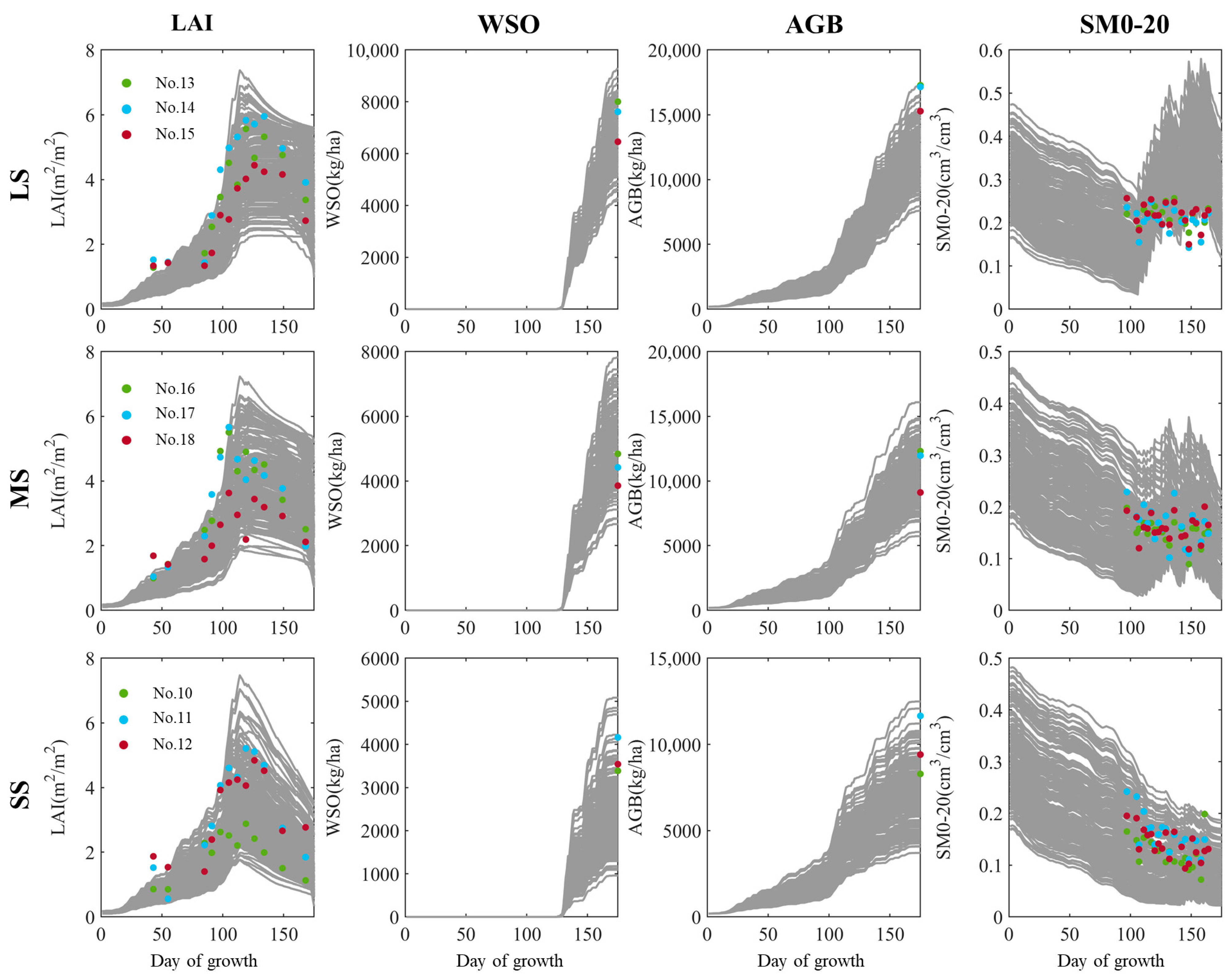
2.3. Site and Data Descriptions

To ensure realistic model uncertainty and the practical relevance of the identified subprocess importance, this study considered a real-world SPAC system simulation scenario. The experiment was conducted at the Irrigation and Drainage Experimental Field of Wuhan University, China (33°33′ N, 114°22′ E). Winter wheat was planted in nine lysimeters from November 2016 to May 2017 under different water conditions. The lysimeters were equipped with rain shelters, and the differences in water supply solely resulted from irrigation management. To ensure successful germination, all lysimeters were watered thoroughly before sowing. Due to weak evapotranspiration during the cold season and the early wheat development, the soil moisture remained sufficient until the end of stem elongation in February 2017. From the booting stage in March 2017 onward, irrigation was required to maintain the soil moisture. The soil water content in the 0–20 cm layer (SM0-20) was measured every three days. Different levels of water stress were set by controlling the soil moisture. Based on literature reviews [32,33,34], irrigation was applied to maintain the soil moisture at 80%, 50%, and 30% of the field capacity (30.81 cm³/cm³), corresponding to the least stress (LS), moderate stress (MS), and severe stress (SS), respectively. A meteorological station was installed next to the lysimeters to record the air temperature, radiation, air humidity, wind speed, and direction at ten-minute intervals. The LAI was measured approximately every one to two weeks, while the grain yield (i.e., WSO) and aboveground biomass (AGB) were collected at harvest. Crop growth stages were recorded following the BBCH scale [35]. As presented in

Table 2. Description of the experimental lysimeters under different water conditions.

	LS	MS	SS
Irrigation Amount (mm)	192.73	72.12	12.50
SM0-20 (cm3/cm3)	$0.21\pm 0.023$	$0.16\pm 0.024$	$0.14\pm 0.028$
Grain Yield (kg/ha)	$7357.84\pm 656.42$	$4371.16\pm 403.34$	$3696.64\pm 334.85$
Lysimeter No.	13, 14, 15	16, 17, 18	10, 11, 12
Growth Stage Duration (days)	emergence: 32; tillering: 58; stem elongation: 15; booting and heading: 24; flowering: 6; grain filling and ripening: 40

, the irrigation treatments effectively modulated the soil moisture conditions, resulting in distinct levels of wheat growth and yields. Within each irrigation treatment, variations among the three lysimeters reflected the natural variability of the SPAC system, which cannot be resolved by a model with deterministic parameter values.

2.4. Implementations

The SWAP model was configured to simulate the experimental SPAC system by localizing as many model components as possible according to field information. Meteorological data and irrigation records were used as model inputs, with each irrigation treatment simulated separately. SWAP simulates crop phenology through the development stage (Dvs), a function of the cumulative temperature sum. Based on the crop calendar and air temperature records, two pivotal model parameters controlling Dvs were determined: TSUMEA, or the temperature sum from emergence (Dvs = 0) to anthesis (Dvs = 1), and TSUMAM, or the temperature sum from anthesis to maturity (Dvs = 2). Other model components were considered uncertain, as they could not be directly determined from observations.

Based on the description in Section 2.1, a total of 36 uncertain parameters (N = 36) were considered in this study, spanning all four subprocesses. Some parameters vary dynamically with the growth stages, such as sla, amax, fl, fo, fs, and fr, which are functions of Dvs. Similarly, rde is a function of the relative soil depth and tmpf is function of the air temperature. Without loss of generality, we assumed uniform distributions for these parameters over their individual variation ranges. To account for the uncertainty existing in the specific experimental SPAC system, this study set the variation ranges using a trial-and-error method. This method ensured that the corresponding distribution of the model simulation captured the observed variability under each water condition. Detailed descriptions and variation ranges for each parameter are given in Table 1.

Focusing on agricultural production, a sensitivity analysis was first performed at the seasonal level. The corresponding seasonal indicators of the five model outputs were set as individual target Y: the maximum LAI, seasonal yield (seasonal WSO), seasonal TW, seasonal SWCC, and seasonal TWCC. Except for the maximum LAI, which occurs at the end of the vegetative period (Dvs = 1), all indicators were evaluated at harvest (Dvs = 2). To further investigate the crop growth dynamics, a sensitivity analysis was also conducted at the growth stage level. Based on the winter wheat phenology [35], the entire growing season was divided into six stages: emergence, tillering, stem elongation, booting and heading, flowering, and grain filling and ripening. The corresponding stage-level indicators for the LAI, WSO, and TW were their respective increments (or decrements) during each stage. For TWCC and SWCC, the corresponding indicators were calculated as increments in CET divided by the increments in TW and WSO during each stage.

To demonstrate the impact of mechanistic interactions between parameters, we also conducted a comparative sensitivity analysis that only considered the importance of individual parameters. For each of the involved parameters, the first-order sensitivity (Equation (5)) was calculated using the method proposed in [29,31]. Specifically, after replicating matrix $\mathcal{A}$, only the column corresponding to that parameter was replaced with the column from matrix $\mathcal{B}$. The sum of the first-order sensitivities of all parameters contained in a subprocess was used as the comparative measure of the subprocess sensitivity, referred to as “Para_sum sensitivity” hereafter for clarity. All sensitivity analyses were performed with 50,000 model simulations, generated from 50,000 randomly sampled parameter sets (K = 50,000). The same parameter sets were used across the simulations for all three water conditions.

3. Results and Discussion

3.1. Examination of the Investigated Simulation Uncertainty

We first examined whether the investigated simulation uncertainty was faithful to the experimental SPAC system. The faithfulness was assessed from two perspectives: (1) Does the uncertainty range sufficiently capture the system’s variability? (2) Do the simulations reasonably reflect the distinct system behaviors under different water conditions?

Figure 2 presents the simulation ensembles for each water condition alongside the corresponding observations. The spread of the grey lines indicates the investigated uncertainty range, while the colored scatter points represent the observed variability in the SPAC system. As shown, all observation values of the measured variables fall within the trajectories of the simulated time series. Moreover, for variables measured throughout the entire growth season (i.e., LAI), the simulated time series ensembles conform well with the observed temporal trends. This suggests that the uncertainty range investigated in this study is sufficiently broad to encompass the potential variability in the SPAC system. At the same time, instead of being unbounded and uncertain, the model simulations considered in this study effectively characterize the system’s dynamics, rather than being arbitrarily dispersed.

Regarding the second aspect, the comparison across the three rows in Figure 2 reveals substantial differences in the simulation ensembles across the three water conditions. First, the overall levels of soil moisture and crop growth (LAI, WSO, and AGB) are highest in LS and lowest in SS, which aligns with the observations (Table 2). Note that the simulations for all three water conditions were generated using the same parameter sets, which aligned with reality as the soil and crop variety remained the same across the treatments. Therefore, the simulation differences were caused by differences in the irrigation inputs. This suggests that the parameter value ranges that we considered allow the model to respond appropriately to varying moisture conditions. There are also differences in the simulated dynamic patterns. For example, in LS, the higher irrigation amount is likely to result in a soil moisture increase, and the crop’s LAI can maintain a high value for a longer period during the middle stage. In contrast, in SS, the soil water content continuously declines and the LAI rapidly decreases after reaching its peak. These differences in both magnitude and temporal patterns confirm that the investigated simulation ensembles serve as a solid foundation for the analysis of the effects of water stress on subprocess importance.

Here, we emphasize that ensuring the faithfulness of the simulation ensembles to the real-world SPAC system is crucial in interpreting sensitivity results as true importance. Many previous works on model parameter sensitivity analysis subjectively preset the parameter variation ranges, without verifying the corresponding model outputs [5,10]. They overlooked the risk that the resultant simulations may not agree with the actual system behavior. The key parameters may be misidentified in this way, as the sensitivity often varies with the variation range due to the high nonlinearity of the underlying processes and the model [36]. However, a broader uncertainty range does not necessarily improve the sensitivity analysis. Expanding the parameter space can increase the spread of the simulation ensemble, but, if certain parameter sets generate unrealistic system dynamics, they can distort the sensitivity calculations and lead to biased importance identification. Therefore, this study carefully balanced the potential model uncertainty and real-world mechanistic characteristics, ensuring that the analyzed uncertainty range was both comprehensive and physically meaningful.

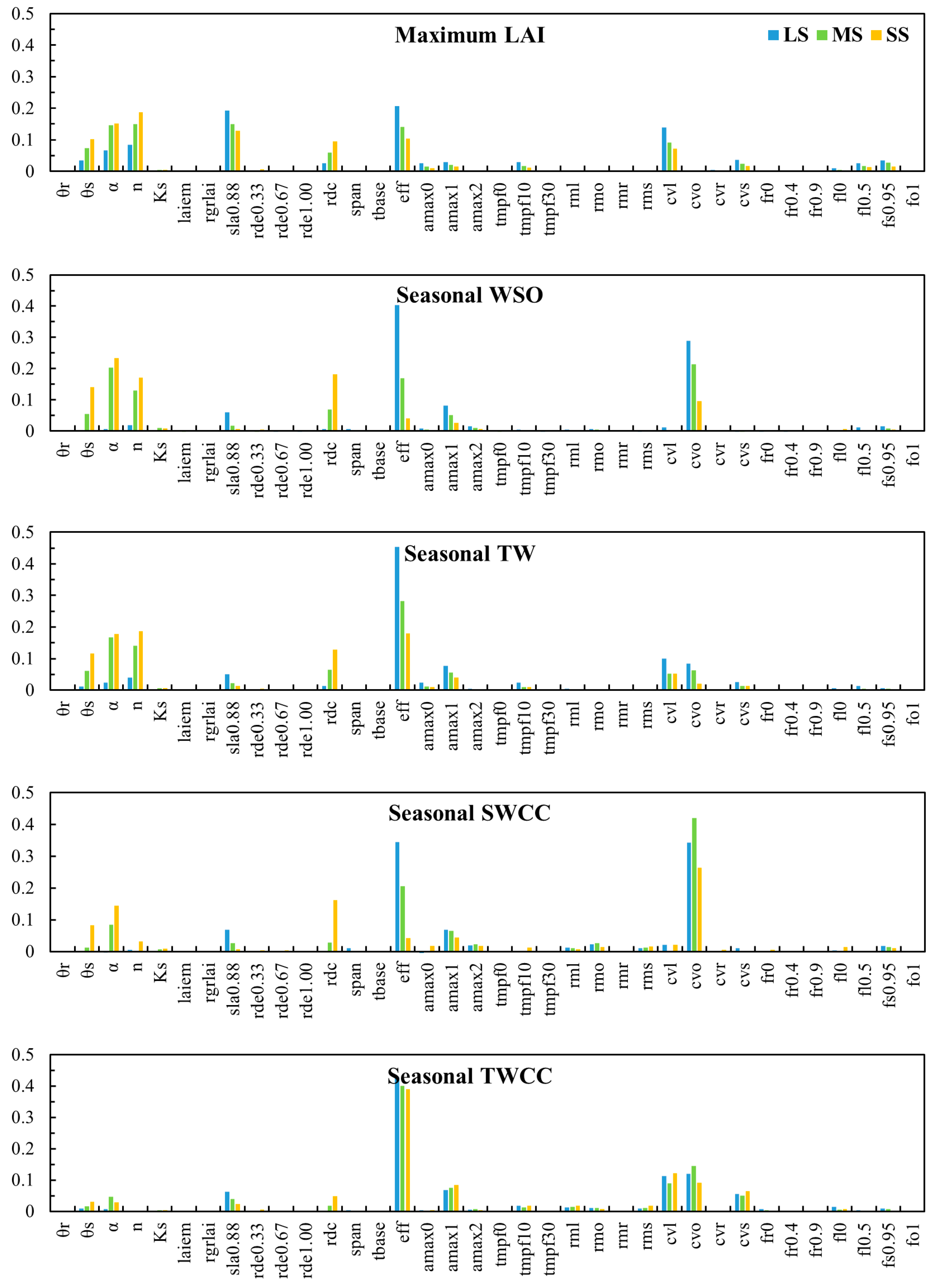
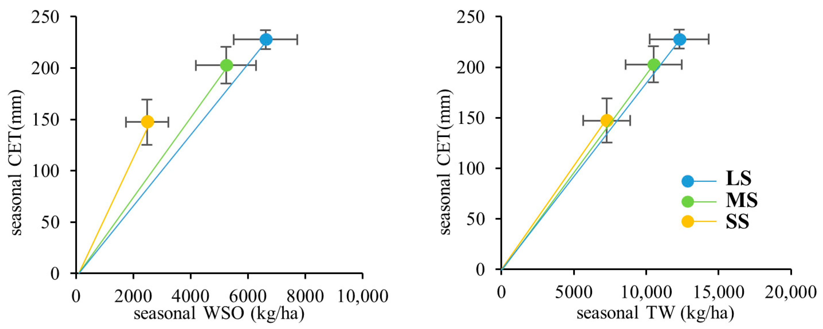
3.2. Impact of Water Stress on Subprocess Importance for Different Seasonal Indicators

Figure 3 shows the subprocess sensitivity results for the maximum LAI and the seasonal WSO, TW, SWCC, and TWCC. Under the LS condition, PPS and PDM, especially PPS, are the most sensitive subprocesses for all seasonal indicators. Their dominance is particularly pronounced for the seasonal WSO, TW, SWCC, and TWCC. For the maximum LAI, PSW and PET also exhibit considerable sensitivity. As the water stress intensifies, the sensitivity of each subprocess for most seasonal indicators shows regular changes. The PPS and PDM sensitivities generally decrease, while the PSW and PET sensitivities increase, with the rise in PSW and the decline in PPS being the most pronounced. This results in the reversal of the subprocess dominance under the SS condition: PSW reaches the highest sensitivity for the maximum LAI and seasonal WSO and TW, while PPS becomes the least sensitive to the maximum LAI and seasonal WSO and SWCC. An exception is the seasonal TWCC, for which the subprocess sensitivity remains largely independent of the water stress.

Agricultural production and the water use efficiency depend on the coupling of water–carbon processes. The four subprocesses defined in this study represent different aspects of this coupling: PSW represents the water process; PPS and PSM represent carbon processes; and PET represents the nexus of water–carbon interactions. Therefore, the above results imply that the dominant factor in water–carbon coupling shifts with changing water conditions. Specifically, under an adequate water supply, crop photosynthesis and dry matter partitioning play the most crucial roles and should be the primary focus of modeling. This is understandable because, in this case, the specific movement of water within the soil does not limit carbon absorption and conversion. Contrarily, when water is severely undersupplied, the specific transport and distribution of soil moisture has a critical impact in terms of supporting crop growth. In this case, the precise modeling of soil water movement is critical for reliable simulations. Root water uptake and evapotranspiration, as the link between soil moisture and plant carbon sequestration, are not negligible under all water conditions but become especially impactful when water is limited. The identified change regularity in the subprocess importance with the water conditions helps to unify the divergent findings of previous studies. For instance, earlier works have reported the low impact of soil parameters under well-irrigated conditions [37], whereas moisture-related parameters were found to be highly influential in dryland environments [38]. This suggests that SPAC system modeling should be adaptive to specific environmental conditions.

It is worth noting that the change regularity of subprocess importance may not be identified if focusing on water use efficiency indicators, especially the water consumption coefficient of all organs (i.e., TWCC). This is because, although different water treatments lead to distinct levels of crop growth, the ratio of biomass accumulation to water use may remain similar, as illustrated in Figure 4. Many existing investigations have also found that, unless the water supply is excessive, the yield and the total biomass increase with the total evapotranspiration in a linear or curvilinear form [39,40,41]. In such a case, the responses of internal components within the SPAC system to water condition changes might be obscured. This underscores the need for multiple perspectives for a comprehensive understanding of the SPAC system.

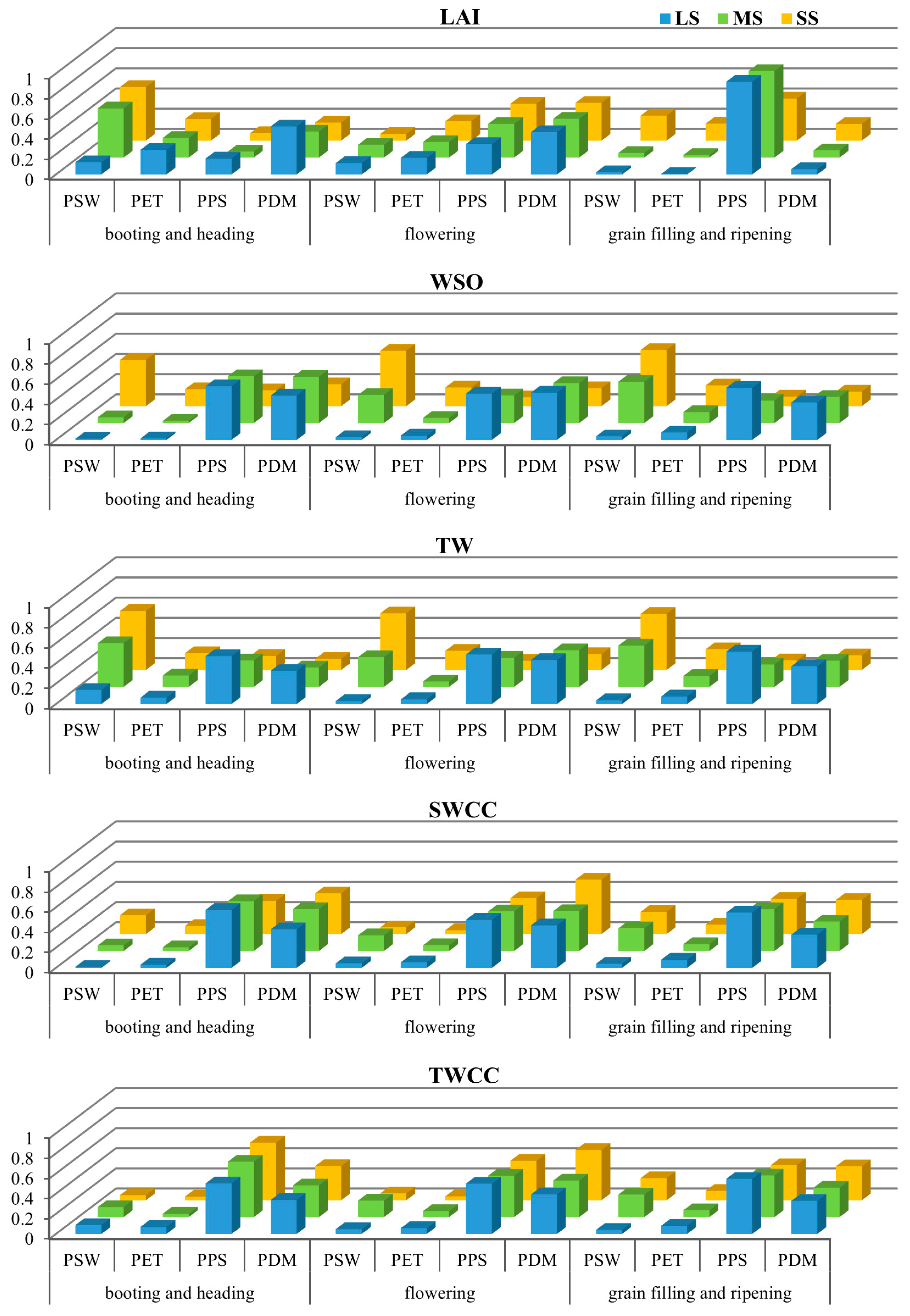
3.3. Impact of Water Stress on Subprocess Importance at Different Growth Stages

The subprocess sensitivity results at different growth stages are presented in Figure 5. Focusing on the influence of water stress, only the stages with different irrigation treatments are included, i.e., from the booting and heading stage to the grain filling and ripening stage.

The initial observation is that, for most model outputs across different growth stages, the subprocess sensitivities still change with the water conditions, and their changes vary from stage to stage. This supports our hypothesis that the subprocess importance is not only influenced by environmental factors but also modulated by the crop phenology. Overall, across all stages, the general trend persists: with the least water stress (LS), PPS and PDM play the dominant role, while, with increasing water stress, PSW and PET gain greater importance. However, whether PSW and PET surpass others to become dominant, as well as how severe the water stress must be to trigger such a shift, appear to be contingent on the physiological demands of the crop at specific growth stages.

For TWCC and SWCC, due to their weaker dependence on the water conditions, the water stress-induced increases in the importance of PSW and PET are very limited. PPS and PDM remain dominant at all growth stages regardless of the water conditions. In contrast, for the LAI, WSO, and TW, severe water stress (SS) can cause PSW to become the dominant subprocess. Specifically, for the LAI, at the booting and heading stage, there is a notable shift in dominance from PDM under LS to PSW under SS. However, at the flowering stage, the changes in subprocess importance due to the water conditions are minor. During the grain filling and ripening stage, the water conditions again have a considerable impact, but PPS remains dominant even under SS. This is understandable, as the canopy is in rapid development during booting and heading, and water sufficiency is critical for the LAI in this stage [42]. In contrast, during flowering, LAI growth ceases, rendering it less sensitive to the water conditions. During grain filling and ripening, leaf senescence is influenced by both the leaf lifespan and drought, explaining why the impact of the water conditions is manifested again but the dominance does not shift to PSW. For WSO and TW, under SS conditions, PSW exhibits the highest importance at all stages. More importantly, the rate of increase in its importance varies across growth stages. During booting and heading, PSW does not gain dominance for WSO until the water supply is severely reduced (SS); however, as growth proceeds, even a moderate water deficit (MS) can lead to PSW dominance. This finding highlights that, from mid-growth onwards, moisture availability becomes increasingly critical for yield formation. This is consistent with the physiological characteristics of winter wheat, as the storage organs begin to develop only after the heading stage [43]. The case for TW is slightly different: during booting and heading, PSW already emerges as the most important subprocess under MS. This is also coherent with the fact that TW contains the biomass of all organs, which develops throughout the growth season.

In summary, these results demonstrate that the proposed sensitivity analysis method is effective and reliable in capturing the dynamic importance of SPAC subprocesses across different crop growth stages under varying water conditions. In addition, the findings reveal that different SPAC system states have different water-critical periods, providing valuable insights for adaptive water resource management.

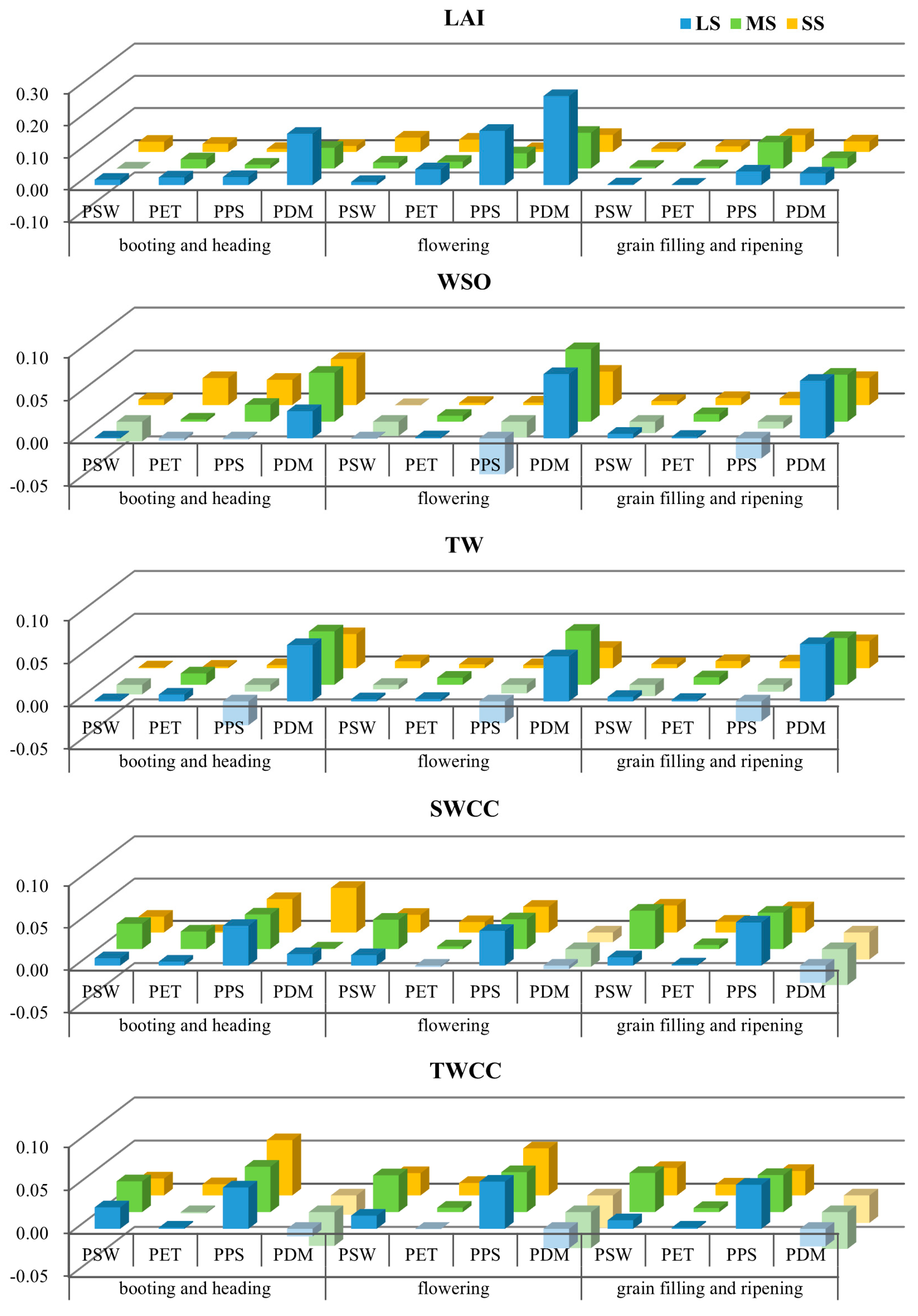
3.4. The Influence of Parameter Interactions on Subprocess Importance Identification

To demonstrate the influence of parameter interactions on the identification of important subprocesses, we compared the subprocess sensitivities calculated by our proposed method with the Para_sum sensitivity. Their differences for individual model outputs at different growth stages are plotted in Figure 6. Positive values indicate that interactions amplify the effect of subprocess uncertainty on the final outputs. Negative values reveal counteracting or overlapping effects of multiple parameters, which, if ignored, can lead to the overestimation of the corresponding subprocess importance. Note that the latter cannot be captured by traditional variance-based methods, as they assign positive values for all terms of single parameters and parameter subsets, thereby predisposing the analysis to an increase in variance when interactions are considered [44]. However, counteracting or overlapping parameter uncertainty can exist in the mechanism. For example, the calculation of the gross CO₂ assimilation rate ($A_{gross}$) is affected by multiple parameters, such as eff, amax, and tmpf. Variations in either eff or amax can introduce uncertainty, yet higher light use efficiency (eff) combined with a lower maximum CO₂ assimilation rate (amax) may jointly cause the outputs to change less. Another typical example exists in PSW, where the soil water retention curve is jointly defined by parameters $\alpha$, n, ${\theta }_S$, and ${\theta }_r$. In Figure 6, negative values corresponding to PPS and PSW can be observed. This illustrates that our proposed sensitivity analysis method can more reasonably assess the subprocess importance by considering the mechanistic relationships between parameters and subprocesses through the BN.

When considering the absolute values of the differences—regardless of their signs—as indicators of a parameter interaction influence, Figure 6 exhibits interpretable patterns. For the LAI, WSO, and TW, interactions between parameters in PPS and PDM play the major role. However, for SWCC and TWCC, parameter interactions in PSW also exhibit strong effects. This can be attributed to the fact that SWCC and TWCC serve as indicators of the water use efficiency and are more directly linked to the simulation of water movement processes. Moreover, under substantial water stress (MS and SS), the impact of PSW parameter interactions on SWCC and TWCC becomes even more pronounced, further supporting this interpretation. Meanwhile, as the crop enters the grain filling and ripening stage, the influence of parameter interactions on the LAI from all subprocesses becomes notably minor. This is likely due to canopy development ceasing during this period, which reduces its dependency on intricate subprocess simulations. These observed patterns, encompassing variations across the model outputs, water conditions, and crop growth stages, align well with known SPAC system mechanisms. This coherence demonstrates the reliability of our proposed subprocess sensitivity analysis method in accounting for parameter interactions.

The advanced subprocess sensitivity provides a macroscopic model understanding beyond the parameter scale and is more instructive for model structure improvement. This can be showcased by two examples. First, as shown in Figure A1, under the least water stress (LS), parameter eff (belonging to PPS) is the overwhelmingly dominant uncertainty contributor for seasonal TW. A conventional parameter sensitivity analysis might focus only on refining PPS. However, the subprocess sensitivity analysis (Figure 3) reveals that PDM accounts for as much as 30% of the total uncertainty, ranking as the second most important subprocess. This exemplifies the advantage of our subprocess sensitivity analysis in identifying important model components that are potentially overlooked by parameter sensitivity. Second, Figure A1 shows that, for the maximum LAI, as the water stress intensifies, the sensitivity of sla0.88 decreases, while the sensitivity of rdc increases. Such divergence makes it challenging to understand how the importance of PET changes with the water conditions. However, the subprocess sensitivity analysis (Figure 3) clearly indicates that PET maintains a nearly constant contribution to the maximum LAI under different water conditions. This further underscores the advantage of our approach in synthesizing the different responses of the parameter sensitivities to provide a holistic understanding of how model components respond to environmental changes.

3.5. Limitations and Outlook

The results and analysis presented above demonstrate the effectiveness and reliability of the proposed sensitivity analysis method in identifying important subprocesses within the SPAC system and revealing their responses to varying water conditions. Nevertheless, the aim is not to replace parameter sensitivity with subprocess sensitivity, but rather to emphasize that conventional parameter sensitivity analysis is insufficient in understanding this complex system. A more comprehensive approach could involve combining both process and parameter sensitivities to understand the importance of system components at multiple levels. This is because the uncertainty in modeling a complex system can arise from both mode conceptualization and parameterization [45,46]. For example, for the temporal evolution of the LAI, the subprocess sensitivities (Figure 5) identify that the influence of PPS grows from negligible to critical as the system progresses from the booting and heading stage to the grain filling and ripening stage. Furthermore, the parameter sensitivities indicate that there is a shift in the factors determining the influence of PPS (Figure A2): before grain filling, capturing the leaves’ photosynthesis intensity is key (parameters eff, amax, tmpf), while, during the grain filling and ripening stage, leaf aging becomes vital (parameter span). In practice, these combined insights provide more comprehensive guidance for the optimization of both the model structure and parameters.

This paper presents a case study to demonstrate the proposed subprocess sensitivity method. Although the SWAP model serves as a useful tool, it cannot fully represent the complexity and uncertainty inherent in SPAC system simulations. While a real-world SPAC system was examined, it remained relatively simple due to the controlled experimental treatments. The subprocess demarcation may differ according to different research interests. The detailed sensitivity results are expected to change with differences in the crop variety, soil characteristics, climate conditions, and field management. Nonetheless, the effectiveness of the proposed method is evident, and its principles are flexible and applicable to a wide range of scenarios.

4. Conclusions

This study proposes a novel subprocess sensitivity analysis method for the SPAC system by integrating the BN framework. Differing from conventional parameter sensitivity analysis, the subprocess sensitivity method further accounts for the mechanistic parameter interactions and subprocess dependencies. Based on a simulation ensemble that faithfully represents the target SPAC system, the subprocess sensitivity results not only guide improvements in model components but also enhance the understanding of subprocess importance within the complex SPAC system. Through an experimental SPAC system with controlled water treatments, several key findings emerge.

(1)

Under minimal water stress, the subprocesses of photosynthesis and dry matter partitioning (PPS and PDM) play the major roles in determining the agricultural outputs and water use efficiency. In this case, uncertainties in modeling the subprocesses of soil water movement and plant water uptake (PSM and PET) have a limited impact. As water becomes increasingly undersupplied, the importance of PSM and PET increases, with PSM becoming the predominant subprocess under sever water stress. This suggests that the water and carbon processes alternately act as limiting factors under variable water conditions.

(2)

The response of the subprocess importance to water stress is modulated by the crop phenology and has different patterns for different SPAC system states. For canopy development (LAI), the water supply has a significant impact during the booting and heading stage and the grain filling and ripening stage, but not during flowering. For the yield (WSO), the water stress threshold required to reverse the dominance of subprocesses decreases as yield formation progresses. For the total biomass (TW), even moderate water stress can lead to significant changes in subprocess importance throughout all growth stages.

(3)

Compared to conventional parameter sensitivity analysis, the proposed subprocess sensitivity analysis offers several advantages: it accounts for the counteracting or overlapping effects of parameter uncertainty, synthesizes the divergent responses of the parameter importance to varying water conditions, and identifies important subprocesses even in the absence of highly sensitive parameters.

Combined with sensitivity analysis at multiple levels, it is expected that the proposed subprocess sensitivity analysis method will contribute to a more comprehensive understanding of SPAC system dynamics and modeling.

References

1. Abrahamsen, P.; Hansen, S. Daisy: An Open Soil-Crop-Atmosphere System Model. Environ. Model. Softw. 2000, 15, 313–330. [Google Scholar] [CrossRef]
2. de Wit, A.; Boogaard, H.; Fumagalli, D.; Janssen, S.; Knapen, R.; van Kraalingen, D.; Supit, I.; van der Wijngaart, R.; van Diepen, K. 25 Years of the WOFOST Cropping Systems Model. Agric. Syst. 2019, 168, 154–167. [Google Scholar] [CrossRef]
3. Bouman, B.; Kropff, M.; Tuong, T.; Wopereis, M.; ten Berge, H.; van Laar, H.H. ORYZA2000: Modeling Lowland Rice; IRRI: Los Baños, Philippines, 2001; ISBN 978-971-22-0171-4. [Google Scholar]
4. Sławiński, C.; Sobczuk, H. Soil–Plant–Atmosphere Continuum. In Encyclopedia of Agrophysics; Gliński, J., Horabik, J., Lipiec, J., Eds.; Springer: Dordrecht, The Netherlands, 2011; pp. 805–810. ISBN 978-90-481-3585-1. [Google Scholar]
5. Makowski, D.; Naud, C.; Jeuffroy, M.H.; Barbottin, A.; Monod, H. Global Sensitivity Analysis for Calculating the Contribution of Genetic Parameters to the Variance of Crop Model Prediction. Reliab. Eng. Syst. Saf. 2006, 91, 1142–1147. [Google Scholar] [CrossRef]
6. Varella, H.; Buis, S.; Launay, M.; Guérif, M. Global Sensitivity Analysis for Choosing the Main Soil Parameters of a Crop Model to Be Determined. Agric. Sci. 2012, 03, 949–961. [Google Scholar] [CrossRef]
7. Sheikholeslami, R.; Razavi, S.; Haghnegahdar, A. What Should We Do When a Model Crashes? Recommendations for Global Sensitivity Analysis of Earth and Environmental Systems Models. Geosci. Model. Dev. 2019, 12, 4275–4296. [Google Scholar] [CrossRef]
8. Razavi, S.; Jakeman, A.; Saltelli, A.; Prieur, C.; Iooss, B.; Borgonovo, E.; Plischke, E.; Lo Piano, S.; Iwanaga, T.; Becker, W.; et al. The Future of Sensitivity Analysis: An Essential Discipline for Systems Modeling and Policy Support. Environ. Model. Softw. 2021, 137, 104954. [Google Scholar] [CrossRef]
9. Zheng, J.; Zhang, S. Decomposing the Total Uncertainty in Wheat Modeling: An Analysis of Model Structure, Parameters, Weather Data Inputs, and Squared Bias Contributions. Agric. Syst. 2025, 224, 104215. [Google Scholar] [CrossRef]
10. Li, X.; Tan, J.; Li, H.; Wang, L.; Niu, G.; Wang, X. Sensitivity Analysis of the WOFOST Crop Model Parameters Using the EFAST Method and Verification of Its Adaptability in the Yellow River Irrigation Area, Northwest China. Agronomy 2023, 13, 2294. [Google Scholar] [CrossRef]
11. Liang, H.; Xu, J.; Chen, L.; Li, B.; Hu, K. Bayesian Calibration and Uncertainty Analysis of an Agroecosystem Model under Different N Management Practices. Eur. J. Agron. 2022, 133, 126429. [Google Scholar] [CrossRef]
12. Jin, X.; Li, Z.; Nie, C.; Xu, X.; Feng, H.; Guo, W.; Wang, J. Parameter Sensitivity Analysis of the AquaCrop Model Based on Extended Fourier Amplitude Sensitivity under Different Agro-Meteorological Conditions and Application. Field Crops Res. 2018, 226, 1–15. [Google Scholar] [CrossRef]
13. Xu, T.; Valocchi, A.J. A Bayesian Approach to Improved Calibration and Prediction of Groundwater Models with Structural Error. Water Resour. Res. 2015, 51, 9290–9311. [Google Scholar] [CrossRef]
14. Gupta, H.V.; Clark, M.P.; Vrugt, J.A.; Abramowitz, G.; Ye, M. Towards a Comprehensive Assessment of Model Structural Adequacy. Water Resour. Res. 2012, 48. [Google Scholar] [CrossRef]
15. Alderman, P.D.; Stanfill, B. Quantifying Model-Structure- and Parameter-Driven Uncertainties in Spring Wheat Phenology Prediction with Bayesian Analysis. Eur. J. Agron. 2017, 88, 1–9. [Google Scholar] [CrossRef]
16. Zhang, S.; Tao, F.; Zhang, Z. Uncertainty from Model Structure Is Larger than That from Model Parameters in Simulating Rice Phenology in China. Eur. J. Agron. 2017, 87, 30–39. [Google Scholar] [CrossRef]
17. Silva, L.C.R.; Lambers, H. Soil-Plant-Atmosphere Interactions: Structure, Function, and Predictive Scaling for Climate Change Mitigation. Plant Soil 2021, 461, 5–27. [Google Scholar] [CrossRef]
18. Kannenberg, S.A.; Barnes, M.L.; Bowling, D.R.; Driscoll, A.W.; Guo, J.S.; Anderegg, W.R.L. Quantifying the Drivers of Ecosystem Fluxes and Water Potential across the Soil-Plant-Atmosphere Continuum in an Arid Woodland. Agric. For. Meteorol. 2023, 329, 109269. [Google Scholar] [CrossRef]
19. Mai, J.; Craig, J.R.; Tolson, B.A. Simultaneously Determining Global Sensitivities of Model Parameters and Model Structure. Hydrol. Earth Syst. Sci. 2020, 24, 5835–5858. [Google Scholar] [CrossRef]
20. Günther, D.; Marke, T.; Essery, R.; Strasser, U. Uncertainties in Snowpack Simulations—Assessing the Impact of Model Structure, Parameter Choice, and Forcing Data Error on Point-Scale Energy Balance Snow Model Performance. Water Resour. Res. 2019, 55, 2779–2800. [Google Scholar] [CrossRef]
21. Baroni, G.; Tarantola, S. A General Probabilistic Framework for Uncertainty and Global Sensitivity Analysis of Deterministic Models: A Hydrological Case Study. Environ. Model. Softw. 2014, 51, 26–34. [Google Scholar] [CrossRef]
22. Sobol, I.M. Global Sensitivity Indices for Nonlinear Mathematical Models and Their Monte Carlo Estimates. Math. Comput. Simul. 2001, 55, 271–280. [Google Scholar] [CrossRef]
23. Darwiche, A. Modeling and Reasoning with Bayesian Networks; Cambridge University Press: Cambridge, UK, 2009; ISBN 978-1-139-47890-8. [Google Scholar]
24. Dai, H.; Chen, X.; Ye, M.; Song, X.; Hammond, G.; Hu, B.; Zachara, J.M. Using Bayesian Networks for Sensitivity Analysis of Complex Biogeochemical Models. Water Resour. Res. 2019, 55, 3541–3555. [Google Scholar] [CrossRef]
25. Kroes, J.G.; Van Dam, J.C.; Groenendijk, P.; Hendriks, R.F.A.; Jacobs, C.M.J. SWAP Version 3.2. Theory Description and User Manual; Alterra: Wageningen, The Netherlands, 2009. [Google Scholar]
26. Heinen, M.; Mulder, M.; van Dam, J.; Bartholomeus, R.; de Jong van Lier, Q.; de Wit, J.; de Wit, A.; Hack-Ten Broeke, M. SWAP 50 Years: Advances in Modelling Soil-Water-Atmosphere-Plant Interactions. Agric. Water Manag. 2024, 298, 108883. [Google Scholar] [CrossRef]
27. Richards, L.A. Capillary Conduction of Liquids Through Porous Mediums. Physics 1931, 1, 318–333. [Google Scholar] [CrossRef]
28. van Genuchten, M.T. A Closed-Form Equation for Predicting the Hydraulic Conductivity of Unsaturated Soils. Soil Sci. Soc. Am. J. 1980, 44, 892–898. [Google Scholar] [CrossRef]
29. Saltelli, A.; Annoni, P.; Azzini, I.; Campolongo, F.; Ratto, M.; Tarantola, S. Variance Based Sensitivity Analysis of Model Output. Design and Estimator for the Total Sensitivity Index. Comput. Phys. Commun. 2010, 181, 259–270. [Google Scholar] [CrossRef]
30. Draper, D.; Pereira, A.; Prado, P.; Saltelli, A.; Cheal, R.; Eguilior, S.; Mendes, B.; Tarantola, S. Scenario and Parametric Uncertainty in GESAMAC: A methodological study in nuclear waste disposal risk assessment. Comput. Phys. Commun. 1999, 117, 142–155. [Google Scholar] [CrossRef]
31. Saltelli, A. Making Best Use of Model Evaluations to Compute Sensitivity Indices. Comput. Phys. Commun. 2002, 145, 280–297. [Google Scholar] [CrossRef]
32. Li, F.; Wei, C.; Zhang, F.; Zhang, J.; Nong, M.; Kang, S. Water-Use Efficiency and Physiological Responses of Maize under Partial Root-Zone Irrigation. Agric. Water Manag. 2010, 97, 1156–1164. [Google Scholar] [CrossRef]
33. Kang, S.; Shi, W.; Zhang, J. An Improved Water-Use Efficiency for Maize Grown under Regulated Deficit Irrigation. Field Crops Res. 2000, 67, 207–214. [Google Scholar] [CrossRef]
34. Cheng, M.; Wang, H.; Fan, J.; Zhang, F.; Wang, X. Effects of Soil Water Deficit at Different Growth Stages on Maize Growth, Yield, and Water Use Efficiency under Alternate Partial Root-Zone Irrigation. Water 2021, 13, 148. [Google Scholar] [CrossRef]
35. Bleiholder, H.; Weber, E.; Lancashire, P.; Feller, C.; Buhr, L.; Hess, M.; Wicke, H.; Hack, H.; Meier, U.; Klose, R. Growth Stages of Mono-and Dicotyledonous Plants. In BBCH Monograph; Federal Biological Research Centre for Agriculture and Forestry: Brunswick, Germany, 2001. [Google Scholar]
36. Wang, J.; Li, X.; Lu, L.; Fang, F. Parameter Sensitivity Analysis of Crop Growth Models Based on the Extended Fourier Amplitude Sensitivity Test Method. Environ. Model. Softw. 2013, 48, 171–182. [Google Scholar] [CrossRef]
37. de Almeida Pereira, R.A.; dos Santos Vianna, M.; Nassif, D.S.P.; dos Santos Carvalho, K.; Marin, F.R. Global Sensitivity and Uncertainty Analysis of a Sugarcane Model Considering the Trash Blanket Effect. Eur. J. Agron. 2021, 130, 126371. [Google Scholar] [CrossRef]
38. Lu, Y.; Chibarabada, T.P.; McCabe, M.F.; De Lannoy, G.J.M.; Sheffield, J. Global Sensitivity Analysis of Crop Yield and Transpiration from the FAO-AquaCrop Model for Dryland Environments. Field Crops Res. 2021, 269, 108182. [Google Scholar] [CrossRef]
39. Hillel, D.; Guron, Y. Relation between Evapotranspiration Rate and Maize Yield. Water Resour. Res. 1973, 9, 743–748. [Google Scholar] [CrossRef]
40. Zhang, X.; Chen, S.; Sun, H.; Shao, L.; Wang, Y. Changes in Evapotranspiration over Irrigated Winter Wheat and Maize in North China Plain over Three Decades. Agric. Water Manag. 2011, 98, 1097–1104. [Google Scholar] [CrossRef]
41. Zhang, Y.; Kendy, E.; Qiang, Y.; Changming, L.; Yanjun, S.; Hongyong, S. Effect of Soil Water Deficit on Evapotranspiration, Crop Yield, and Water Use Efficiency in the North China Plain. Agric. Water Manag. 2004, 64, 107–122. [Google Scholar] [CrossRef]
42. Zhao, F.-H.; Yu, G.-R.; Li, S.-G.; Ren, C.-Y.; Sun, X.-M.; Mi, N.; Li, J.; Ouyang, Z. Canopy Water Use Efficiency of Winter Wheat in the North China Plain. Agric. Water Manag. 2007, 93, 99–108. [Google Scholar] [CrossRef]
43. Ercoli, L.; Lulli, L.; Mariotti, M.; Masoni, A.; Arduini, I. Post-Anthesis Dry Matter and Nitrogen Dynamics in Durum Wheat as Affected by Nitrogen Supply and Soil Water Availability. Eur. J. Agron. 2008, 28, 138–147. [Google Scholar] [CrossRef]
44. Saltelli, A.; Tarantola, S. On the Relative Importance of Input Factors in Mathematical Models: Safety Assessment for Nuclear Waste Disposal. J. Am. Stat. Assoc. 2002, 97, 702–709. [Google Scholar] [CrossRef]
45. Chapagain, R.; Remenyi, T.A.; Harris, R.M.B.; Mohammed, C.L.; Huth, N.; Wallach, D.; Rezaei, E.E.; Ojeda, J.J. Decomposing Crop Model Uncertainty: A Systematic Review. Field Crops Res. 2022, 279, 108448. [Google Scholar] [CrossRef]
46. Wallach, D.; Thorburn, P.J. Estimating Uncertainty in Crop Model Predictions: Current Situation and Future Prospects. Eur. J. Agron. 2017, 88, A1–A7. [Google Scholar] [CrossRef]
Figure 1. The Bayesian network of the SPAC system (based on SWAP). Parameters are placed in ellipses, while intermediary variables and model outputs are in rectangles. Each subprocess is highlighted using shaded regions of different colors. Dashed arrows indicate iterative updates.
Agronomy 15 00753 g001
Figure 2. Simulation uncertainty for LAI, WSO, AGB, and SM0-20 under LS, MS, and SS conditions. The grey lines are instantiations of simulated time series. The colored dots denote observed values.
Agronomy 15 00753 g002
Figure 3. Subprocess sensitivities for maximum LAI, seasonal WSO, seasonal TW, seasonal SWCC, and seasonal TWCC under LS, MS, and SS conditions.
Agronomy 15 00753 g003
Figure 4. Scatterplots showing the relationship between the mean values of seasonal CET, WSO, and TW under LS, MS, and SS conditions. The slopes of the lines passing through the origin represent the mean seasonal water consumption coefficients for each water condition.
Agronomy 15 00753 g004
Figure 5. Subprocess sensitivities for five outputs at different growth stages (from booting and heading to grain filling and ripening) under LS, MS, and SS conditions.
Agronomy 15 00753 g005
Figure 6. Differences in subprocess sensitivity values between our proposed method and the Para_sum sensitivity at different growth stages (from booting and heading to grain filling and ripening) under LS, MS, and SS conditions. Positive values indicate that our method yields higher sensitivity estimates, while negative values suggest lower estimates. For clarity, bars representing negative values are displayed with increased transparency.
Agronomy 15 00753 g006