A Lightweight Model for Shine Muscat Grape Detection in Complex Environments Based on the YOLOv8 Architecture

Abstract

Automated harvesting of “Sunshine Rose” grapes requires accurate detection and classification of grape clusters under challenging orchard conditions, such as occlusion and variable lighting, while ensuring that the model can be deployed on resource- and computation-constrained edge devices. This study addresses these challenges by proposing a lightweight YOLOv8-based model, incorporating DualConv and the novel C2f-GND module to enhance feature extraction and reduce computational complexity. Evaluated on the newly developed Shine-Muscat-Complex dataset of 4715 images, the proposed model achieved a 2.6% improvement in mean Average Precision (mAP) over YOLOv8n while reducing parameters by 36.8%, FLOPs by 34.1%, and inference time by 15%. Compared with the latest YOLOv11n, our model achieved a 3.3% improvement in mAP, with reductions of 26.4% in parameters, 14.3% in FLOPs, and 14.6% in inference time, demonstrating comprehensive enhancements. These results highlight the potential of our model for accurate and efficient deployment on resource-constrained edge devices, providing an algorithmic foundation for the automated harvesting of “Sunshine Rose” grapes.

1. Introduction

Grape harvesting is a critical component in the development of the grape industry. Currently, harvesting is primarily conducted manually, which requires substantial labor, incurs high costs, and is relatively slow. With the progression of urbanization, the agricultural workforce has been steadily declining [1]. As a result, research on grape-harvesting robots has become increasingly significant. Accurate detection of grape clusters is the cornerstone of automated harvesting [2]. However, in the complex environment of vineyards, factors such as lighting variations, changes in distance, leaf occlusion, and overlapping grape clusters pose significant challenges for harvesting robots [3]. During the ripening period, physical damage and infectious diseases, such as gray mold and white rot, can lead to grape decay [4]. Considering the substantial economic disparity between healthy and damaged grape clusters [5], healthy clusters can be directly used for sales and processing, while damaged clusters require additional handling. Furthermore, mixing healthy and damaged clusters during harvesting can exacerbate the spread of disease. Notably, it is not necessary to determine the specific cause of damage during harvesting but rather to identify whether the cluster is damaged [6]. Consequently, the automated sorting of grape clusters into healthy and damaged categories during harvesting holds significant practical implications. This study aims to address these challenges by developing a lightweight and highly accurate object detection and classification model tailored for “Sunshine Rose” grapes in complex agricultural environments. By paving the way for fully automated harvesting with advanced algorithms, this research has significant implications for enhancing the economic viability of “Sun-shine Rose” grape production [7]. Furthermore, the proposed lightweight model can be directly applied in real-world agricultural environments, enabling automated sorting and harvesting of grape clusters. This advancement addresses labor shortages and promotes the application of deep learning models in the field of automated harvesting driving innovation in modern agricultural practices.

Extensive research has been conducted on grape detection, focusing on various traditional and machine learning approaches. For instance, Chamelat et al. [8] utilized Zernike moments and Support Vector Machines (SVMs) for color feature extraction, achieving a recognition error rate below 0.5%. Liu et al. [9], by analyzing the color and texture information of grapes, attained an 88.0% accuracy in detecting grape clusters using SVM. The adoption of deep learning has further advanced grape detection. Cecotti et al. [10] demonstrated the effectiveness of transfer learning with ResNet, highlighting the potential of pre-trained frameworks for achieving high accuracy. Despite these advancements, many existing models are optimized for controlled conditions and may not generalize well to complex orchard environments. Among various deep learning frameworks, the YOLO model is renowned for its balanced performance in speed, efficiency, and accuracy, making it widely applicable across diverse domains. For instance, Zhang, C. et al. [11] implemented YOLOv5 for grape detection, reaching a good level of performance under simple conditions. Although the accuracy of detection models has markedly improved, the computational resources required for inference have also escalated, posing significant challenges for edge devices with limited storage and processing capabilities. As a result, there has been growing interest in research aimed at model lightweighting. Mai et al. [12] significantly improved the detection performance for overlapping and occluded fruits by expanding the single classifier in the Faster R-CNN frameworks to three classifiers. Furthermore, Su Shuzhi et al. [13] introduced a network architecture based on Uniformer, which showed superior performance compared with similar YOLO detection methods at the same scale. Ghiani et al. [14] developed a grape cluster detector based on Mask R-CNN, which achieved relatively good performance on both the GrapeCS-ML dataset and their internal dataset. However, the authors noted that the model struggled with overlapping clusters, small targets at long distances, variations in lighting, and images containing a large number of grape clusters. Sozzi et al. [15] evaluated multiple versions of the YOLO framework for detecting white grape clusters and found that the similarity in color between grape clusters and the background, as well as leaf occlusion, significantly reduced the model’s performance. Building on the limitations of previous studies and the practical requirements of grape cluster detection, we selected “Sunshine Rose” grapes, which share a similar color with their background, as the target of our research. To address these challenges, we constructed a new dataset designed for complex scenarios, incorporating diverse lighting conditions, varying degrees of leaf and cluster occlusion, and a range of distances and angles. Compared with related studies, our detection targets exhibit greater morphological variability, and the detection environments are significantly more complex. Clearly, our research poses greater challenges and holds the potential to advance the state of automated grape cluster detection.

There has been some related research on the classification of healthy and damaged grapes. However, most studies have focused on identifying specific diseases in grape leaves [16], which can help prevent the spread of diseases but cannot fully address the issue of damaged grapes during harvesting. Notably, during the harvest, it is only necessary to distinguish whether the grapes are damaged, rather than identifying the specific cause of the damage. Consequently, some studies have focused on identifying damaged grapes during the ripening period [17], demonstrating the feasibility of distinguishing damaged grapes at the time of harvest. Nevertheless, these studies are limited to simple classifications under ideal conditions and cannot be directly applied to the complex and precise localization scenarios required for automated harvesting. Further research is needed to address these challenges. Therefore, our study aims to classify “Sunshine Rose” grapes into two categories: “Standard Grapes” and “Compromised Grapes”.

The improvement in detection precision has also increased parameters (Params), FLOPs, and inference time. To tackle these challenges while enhancing detection accuracy, F. Chollet et al. [18] introduced depthwise separable convolutions to replace standard convolutions, achieving a 70% reduction in Params and doubling inference speed. Zeng et al. [19] utilized a lightweight convolutional neural network architecture to replace the YOLOv5 backbone for tomato detection, reducing Params and increasing speed while retaining some of YOLO’s high-precision features. Similarly, Cui et al. [20] improved detection speed by substituting the CSPDarknet-Tiny backbone with ShuffleNet and consolidating three detection heads into a single head.

The task of detecting “Sunshine Rose” grapes presents unique challenges due to the close color resemblance between the grapes and their natural background, as well as difficulties caused by dense growth patterns, overlapping fruits, and shadow effects. In practical harvesting scenarios, grapes are sorted by quality. However, most existing studies have focused solely on detecting grapes without addressing quality-based classification, which limits the alignment of these studies with actual agricultural practices. To address this gap, our study introduces a new dataset that classifies “Sunshine Roses” into two classes: “Standard Grapes” and “Compromised Grapes”. The classification can often depend on the quality of an individual fruit, making the task particularly complex. When tested with the YOLOv8n model, our dataset achieved a mean Average Precision (mAP) of only 81.2%, a performance generally lower than that observed in other fruit detection studies, highlighting the challenging nature of this research.

In recent years, the YOLO architecture has emerged as a leading framework in the field of object detection. Its end-to-end advantages enable it to perform effectively across various detection tasks while balancing accuracy with efficient data processing. This study addresses the challenges posed by dense, overlapping, and small targets of “Sunshine Rose” grapes in our complex dataset by proposing a model that is fast, lightweight, and capable of effectively handling intricate scenarios. Specifically, we replace the conventional C2f module with our innovative C2f-GND module in the YOLOv8 framework. Our enhancements to the YOLOv8 model include the following three key improvements:

• Replacing standard convolutions with DualConv leads to a substantial reduction in computational costs and the number of Params.
• Enhancing the C2f module with the Ghost Module maintains model accuracy while greatly reducing the number of Params and FLOPs.
• Integrating Dynamic Convolution into the C2f module enables the model to dynamically adjust convolution kernels for new scenes and adapt to varying lighting conditions and angles.

While numerous CNN-based algorithms have been developed for grape detection, few are specifically tailored for the identification of “Sunshine Roses”, and even fewer address both detection and classification simultaneously. The high-quality Shine-Muscat-Complex dataset we constructed more accurately reflects real-world scenarios and aligns better with our research objectives, presenting greater challenges for detection. Our proposed end-to-end lightweight object detection algorithm demonstrates strong performance on this dataset, ensuring accurate detection of “Sunshine Roses” while meeting the basic requirements for deployment on edge computing devices, thereby providing algorithmic support specifically for the automated harvesting of “Sunshine Rose” grapes.

2. Materials and Methods

This study employs the “Sunshine Rose” grape object detection dataset as the experimental subject. The images in this dataset were captured on 28 and 29 August 2024, between 9:00 a.m. and 3:00 p.m., under natural lighting conditions in a greenhouse located at the Xianlu Island Shared Grape Harvesting Garden in Foshan City (Longitude: 113.1° E, Latitude: 23.2° N). The local climate during this period was characterized by warm temperatures and high humidity, typical of the subtropical region. The daytime temperature ranged from 28 °C to 35 °C, with humidity levels between 70% and 85%. These conditions, combined with the controlled environment of the greenhouse, created an optimal setting for grape growth. The greenhouse helped to protect the crops from extreme weather conditions, such as heavy rainfall and strong winds, while maintaining a stable microclimate conducive to high-quality grape development. The controlled temperature and humidity levels inside the greenhouse ensured consistent conditions for the growth of the Sunshine Rose variety.

To ensure that the dataset captures diverse real-world scenarios and enhance the model’s generalization ability, images were taken using different devices, including an iPhone 13 (Apple Inc., Cupertino, CA, USA) and a Huawei Mate 40 Pro (Huawei Technologies Co., Ltd., Shenzhen, China), under various shooting angles. For frontal and low-angle shots, the distance between the camera and the grape clusters was approximately 0.5 to 2 m. For parallel shots, which aimed to replicate field-level observations, the distance was variable and not precisely measurable due to the shooting geometry.

This dataset focuses on Shine Muscat grapes. These grapes are characterized by elliptical or round berries that are plump and uniformly shaped, with minimal visible defects. The fruit surface is yellow-green, with consistent coloration throughout the cluster and little variation. The clusters are typically cylindrical or conical, measuring 16 to 20 cm in length, with a smooth and uniform transition in shape, and no missing or protruding berries. The berries are arranged in a single layer, showing no visible compression or deformation, and are loosely and appropriately attached. The pedicel is soft, the peduncle is fresh, and the pedicel color ranges from green to yellow-green.

We captured a total of 1049 images. After cleaning and cropping, 943 images with a resolution of 1280 × 1280 pixels were retained. Manual annotation was performed using LabelImg, categorizing the images into two classes: “Standard Grapes” and “Compromised Grapes”. The annotation format followed the YOLO standard. To ensure annotation quality, the following guidelines were followed:

• Grape clusters that appear blurry were not annotated.
• Grape clusters that are more than two-thirds obscured were not annotated.
• Grape clusters that have not been de-bagged were not annotated.
• Annotation boxes were drawn to enclose grape clusters as completely as possible.

2.1. Data Preprocessing and Augmentation

To enhance the applicability of this study, the data processing phase involved categorizing grapes into two classes: “Standard Grapes” and “Compromised Grapes”. “Standard Grapes” are visually appealing clusters with uniform coloration, intact fruits, and no signs of physical damage or decay. In contrast, “Compromised Grapes” are clusters that display clear defects, such as blackened, moldy, or damaged fruits, which are indicative of reduced quality. In real-world scenarios, grape clusters are often densely packed, leading to challenges such as occlusion, overlap, and uneven lighting, which complicate the detection and classification of “Sunshine Rose” grapes.

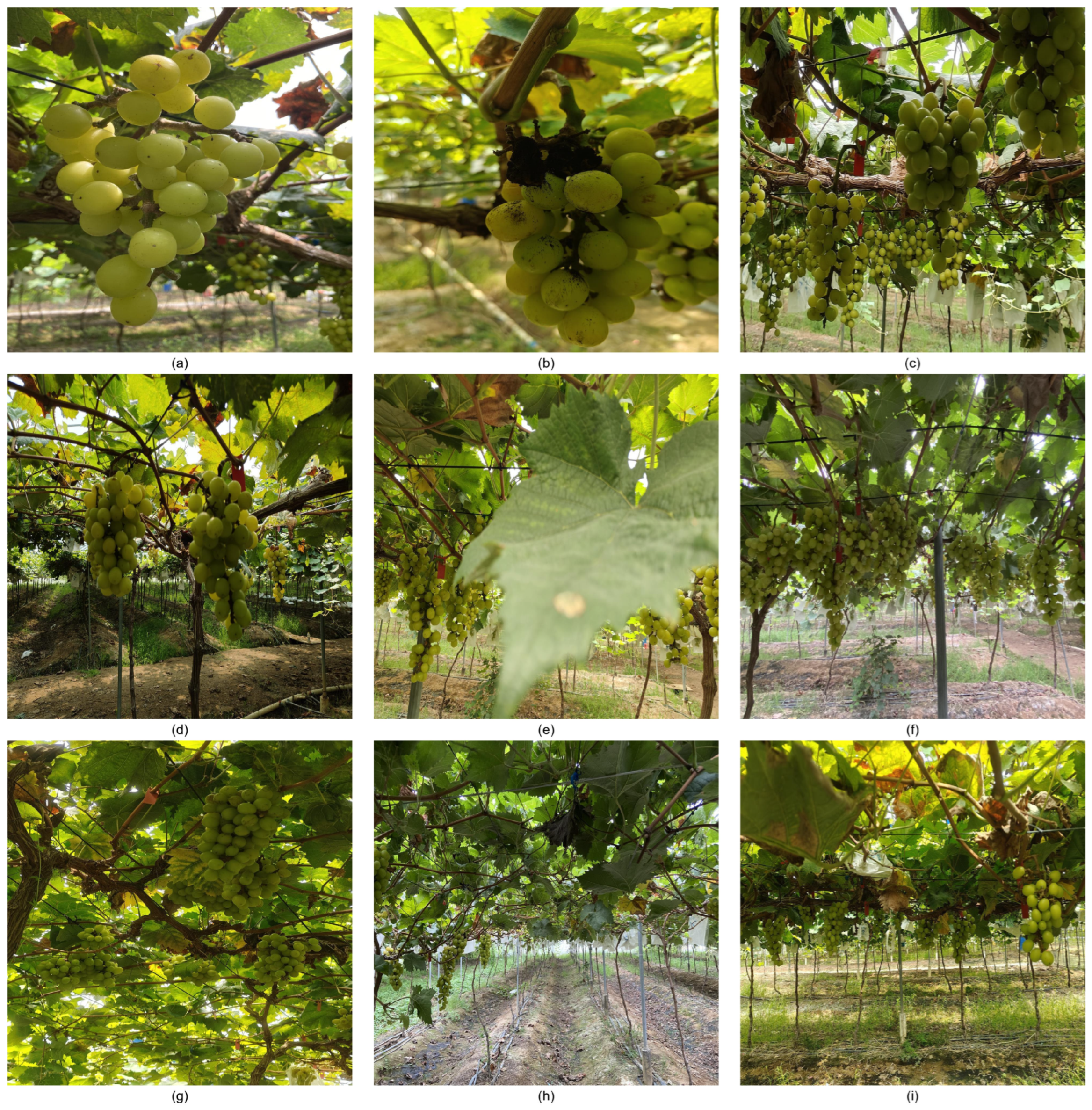
To ensure effective learning from complex real-world scenarios and prevent overfitting, we employed a multi-faceted, multi-angle approach during data acquisition. This strategy aims to enhance the model’s robustness by capturing diverse scenarios. The dataset was categorized into nine different conditions: “Standard Grapes”, “Compromised Grapes”, multiple grape clusters, varying lighting conditions, leaf occlusion, fruit occlusion, low-angle capture, parallel capture, and frontal capture. Representative samples are shown in Figure 1.

Furthermore, to enrich the dataset and enhance the model’s generalization capability, we applied various data augmentation techniques to the original images, including rotation to simulate various capture angles in real orchard environments, noise addition to emulate sensor noise and environmental interferences, and image blurring to mimic motion blur caused by wind or camera movement. These augmentations helped ensure that the model could effectively detect grape clusters regardless of orientation, variations in image quality, or imperfect clarity. This process resulted in the creation of the Shine-Muscat-Complex dataset, consisting of 4715 valid images, as shown in Figure 2. To ensure the rigor of the study, the dataset was randomly divided into training, validation, and testing sets at a ratio of 7:2:1.

2.2. Architecture Detail of Our Network

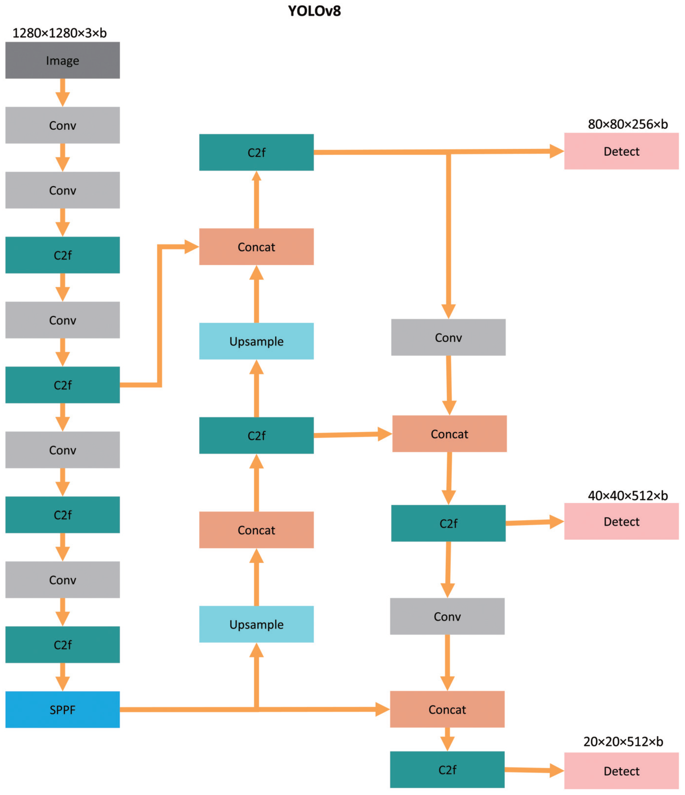
YOLOv8 [21] is an object detection network developed by the Ultralytics team and released in January 2023. Building on the advancements of earlier YOLO models, YOLOv8 introduces several new features that enhance both its efficiency and accuracy in object detection tasks. The architecture of YOLOv8 consists of three main components: Backbone, Neck, and Head. For our research, we selected YOLOv8n as the foundational model to optimize deployment on edge computing devices while ensuring high performance. 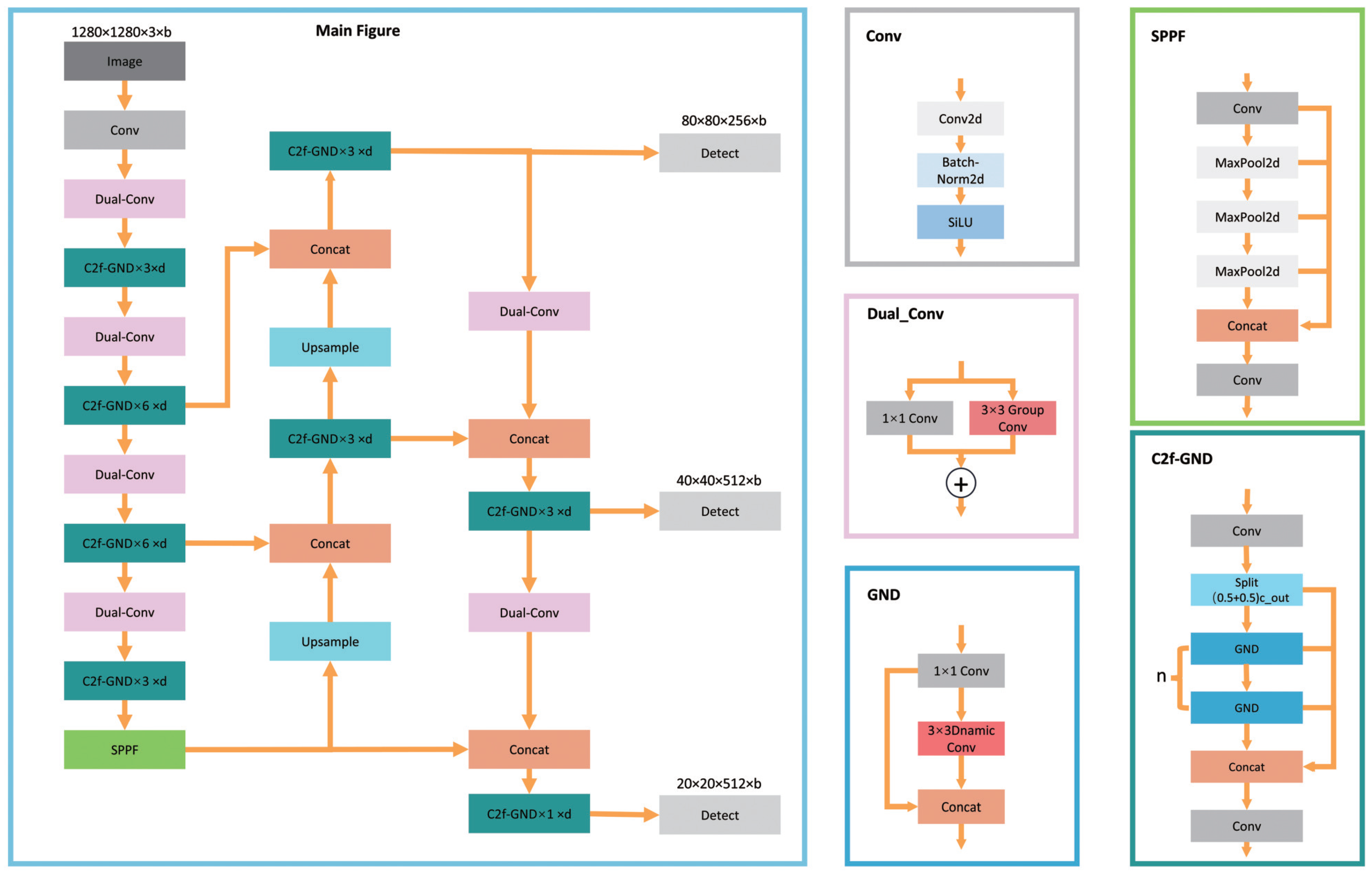As shown in Figure 3, the original YOLOv8 utilizes C2f modules and standard convolution layers throughout its Backbone and Neck. In our improved network, illustrated in Figure 4, the C2f modules are replaced with C2f-GND, which introduces a GND Bottleneck controlled by a key hyperparameter d, allowing dynamic adjustments to the network’s capacity and depth. Additionally, the standard convolution layers are replaced with DualConv modules, which enhance feature extraction and gradient flow through dual convolution operations. These modifications collectively improve the network’s adaptability, accuracy, and efficiency, enabling robust detection and classification of “Sunshine Rose” grapes under complex environmental conditions.

The Backbone of YOLOv8 incorporates an improved version of the CSPDarknet53 network, which builds upon the original Darknet53. Unlike YOLOv5, YOLOv8 utilizes a more lightweight C2f module to replace the C3 module used in YOLOv5, maintaining a lightweight architecture while enhancing gradient flow. At the end of the Backbone, YOLOv8 includes the Spatial Pyramid Pooling-Fast (SPPF) module, an efficient information fusion module ideal for edge devices. In our research, we replaced the C2f module with our custom C2f-GND module, substituting the Bottleneck with the Ghost Module architecture [22]. A 1 × 1 convolution is used to control the number of input feature map channels, producing a lighter set of output feature maps. Subsequently, low-cost depthwise convolutions are applied to generate Ghost feature maps, allowing our model to maintain a low number of FLOPs and Params while retaining effective feature extraction for “Standard Grapes” and “Compromised Grapes”. These feature maps are then concatenated for further processing. By incorporating the Ghost Module, our model achieves a 28% reduction in FLOPs and a 30.5% decrease in Params. While there is a minor compromise in feature extraction capability, the overall performance of the model is maintained or slightly improved. This modification strikes a balance between efficient feature extraction and model lightweighting, addressing the challenge of deploying lightweight models for our task. The C2f module is a pivotal part of the Backbone, crucial for feature extraction efficiency, as it significantly impacts the distribution of FLOPs and Params and contributes to the model’s expressiveness. To balance efficiency with adaptability, we designed the C2f-GND module to use Dynamic Convolution [23] in place of standard convolution. This approach enhances the model’s generalization capabilities, making it better suited for resource-constrained environments.

Given the resource constraints of many edge computing devices, we aimed to further reduce the weight of our model while preserving its accuracy. Dual Convolution [24] integrates the strengths of Group Convolution (GroupConv) [25] and Heterogeneous Convolution (HetConv) [26], optimizing both feature extraction and information processing to enhance model efficiency and performance. GroupConv processes only a subset of input channels at a time, which effectively lowers the computational cost of convolution operations. Replacing standard convolutions with Dual Convolution significantly reduced computational cost and the number of Params, while maintaining or even improving model performance.

2.3. Principles of Model Improvements

2.3.1. Ghost Module

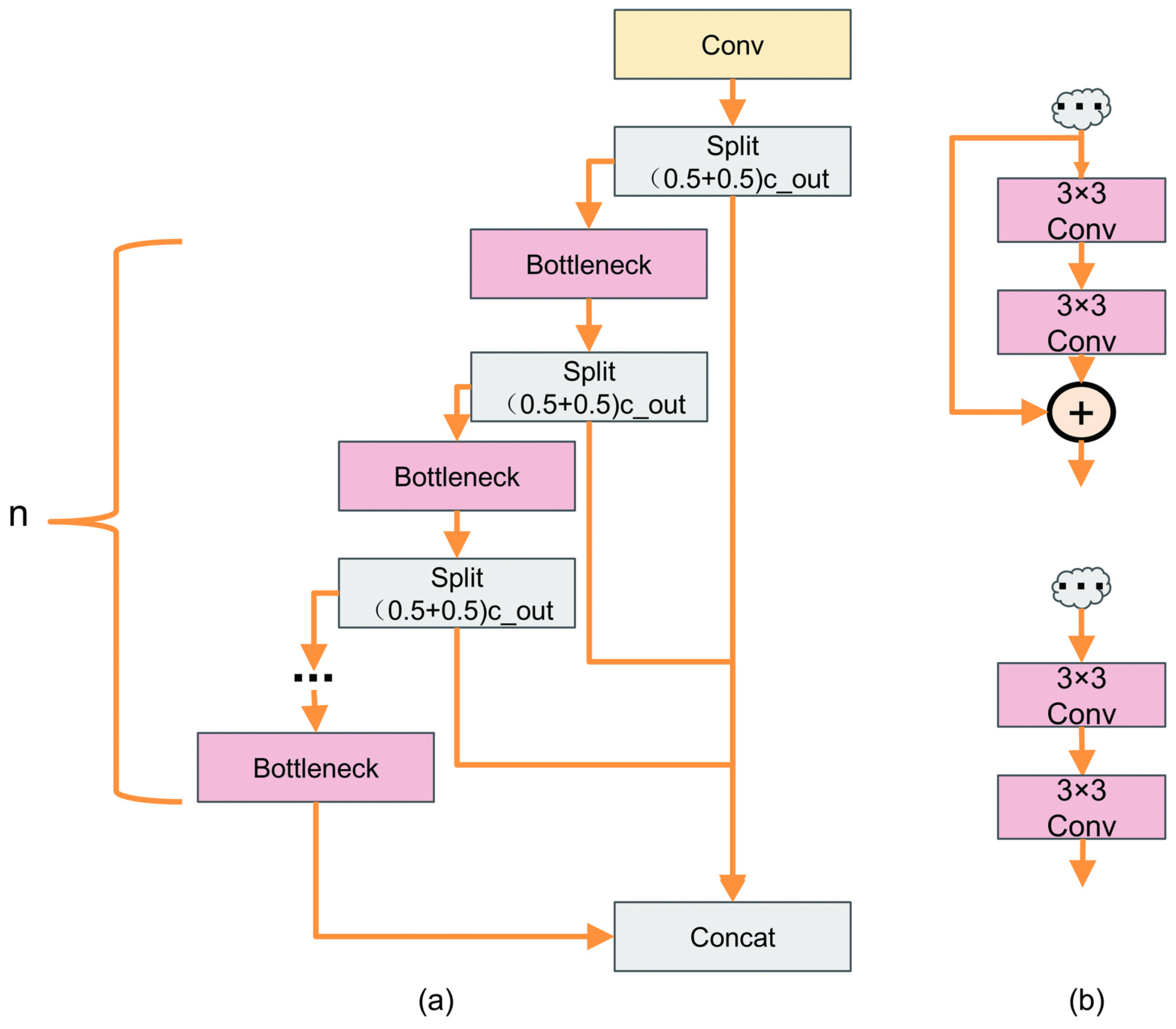
The C2F module in YOLOv8 represents an advancement over the C3 module used in YOLOv5, as shown in Figure 5a. Figure 5b illustrates two different cases of the Bottleneck. In Figure 5b, the Bottleneck block processes the input feature map through two standard 3 × 3 convolutions. If the shortcut is set to True, the residual connection is added to the output feature map. If the shortcut is set to False, the output is generated directly without the addition of the residual. Unlike the C3 module, the C2F block incorporates more skip connections, removes convolution operations within the branches, and introduces additional split operations. This design enhances the module’s ability to capture more comprehensive feature information.

The C2F module is essential for learning and utilizing the correlations between features, thereby enhancing the model’s feature extraction capabilities. It is a critical component that is repeatedly stacked, significantly impacting the model’s mAP, Params, and FLOPs. To maximize the benefits of this module in feature extraction while minimizing the substantial computational burden of frequent convolutions, we have enhanced the C2F module by replacing its Bottleneck with a Ghost Module. This modification aims to reduce the model size and lower deployment costs, embodying our design principles for a lightweight network architecture. The Ghost Module, as shown in Figure 6, replaces standard convolutions with Ghost Convolutions to achieve this efficiency.

Structurally, the Ghost Module closely resembles the traditional Bottleneck, but it replaces standard convolutions with Ghost Convolutions. When the shortcut connection is enabled ($\mathrm{shortcut}=\mathrm{True}$), the input feature map $\mathbf{x}$ is first processed by a $1\times 1$ convolution to produce the following ${\mathbf{x}}_{\mathbf{1}}$:

$${\mathbf{x}}_{\mathbf{1}}=\sigma ({\mathbf{W}}_{1\times 1}\ast \mathbf{x}),$$

(1)

where ${\mathbf{W}}_{1\times 1}$ is the weight matrix of the $1\times 1$ convolution, and $\sigma$ denotes the activation function (e.g., ReLU). Next, ${\mathbf{x}}_{\mathbf{1}}$ undergoes a $3\times 3$ depthwise convolution to generate the following ${\mathbf{x}}_{\mathbf{2}}$:

$${\mathbf{x}}_{\mathbf{2}}=\sigma ({\mathbf{W}}_{\mathrm{dw}}\ast {\mathbf{x}}_{\mathbf{1}}),$$

(2)

where ${\mathbf{W}}_{\mathrm{dw}}$ is the weight matrix of the depthwise convolution. Finally, the output feature map ${\mathbf{x}}_{\mathrm{out}}$ is obtained by concatenating the following ${\mathbf{x}}_{\mathbf{1}}$ and ${\mathbf{x}}_{\mathbf{2}}$:

$${\mathbf{x}}_{\mathrm{out}}={\mathbf{x}}_{\mathbf{1}}\oplus {\mathbf{x}}_{\mathbf{2}},$$

(3)

where ⊕ denotes the concatenation operation. This concatenation ensures the preservation of critical feature information while minimizing redundancy.

Unlike the two $3\times 3$ standard convolutions in the Bottleneck, which directly extract image features, the Ghost Convolution employs a single $1\times 1$ convolution to control the number of channels, eliminating redundant information while retaining essential features to produce the feature map ${\mathbf{y}}_{\mathbf{1}}$. Subsequently, applying a depthwise convolution on ${\mathbf{y}}_{\mathbf{1}}$ generates the feature map ${\mathbf{y}}_{\mathbf{2}}$, which, when concatenated with ${\mathbf{y}}_{\mathbf{1}}$, results in ${\mathbf{x}}_{\mathbf{2}}$.

In comparative experiments, we observed that the first standard convolution in a Bottleneck generates 4640 parameters, while the Ghost Module utilizing Ghost Convolutions reduces this count to just 216 parameters, representing a reduction of 95.3%. Overall, the parts replaced by the Ghost Module typically experience a parameter reduction of 90% to 95%.

While the standard convolution operation in the Bottleneck effectively extracts features from images, Han et al. observed that many features can be obtained through multiple simple linear transformations, reducing the need for all feature maps to undergo the nonlinear transformations inherent in standard convolutions. The Bottleneck employs two $3\times 3$ standard convolutions to generate multiple channels of feature maps, retaining positional information through feature fusion. In contrast, our Ghost Module introduces a potential risk of losing some target feature information. To address this, we incorporate a depthwise convolution after the $1\times 1$ standard convolution in the Ghost Module, enabling low-cost linear processing. By concatenating the resulting outputs, we ensure there is no significant loss of critical feature information.

In summary, despite the reductions in Params and FLOPs, the feature maps generated by Ghost Convolutions are comparable to those produced by standard convolutions, allowing us to maintain robust feature extraction capabilities while decreasing the model’s FLOPs and Params.

2.3.2. Dynamic Convolution

Utilizing the Ghost Module to lightweight our model effectively reduces the number of Params and FLOPs, making it more suitable for deployment on resource-constrained devices. However, this reduction in Params can also lead to a decrease in model accuracy, as a higher number of trainable Params typically enhance model expressiveness. This perspective is supported by Han et al. [27], which, while focusing on large-scale visual pretraining, highlights the importance of Params in maintaining high accuracy.

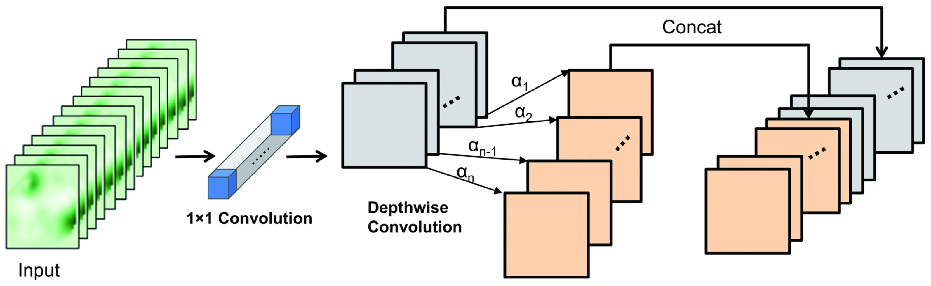
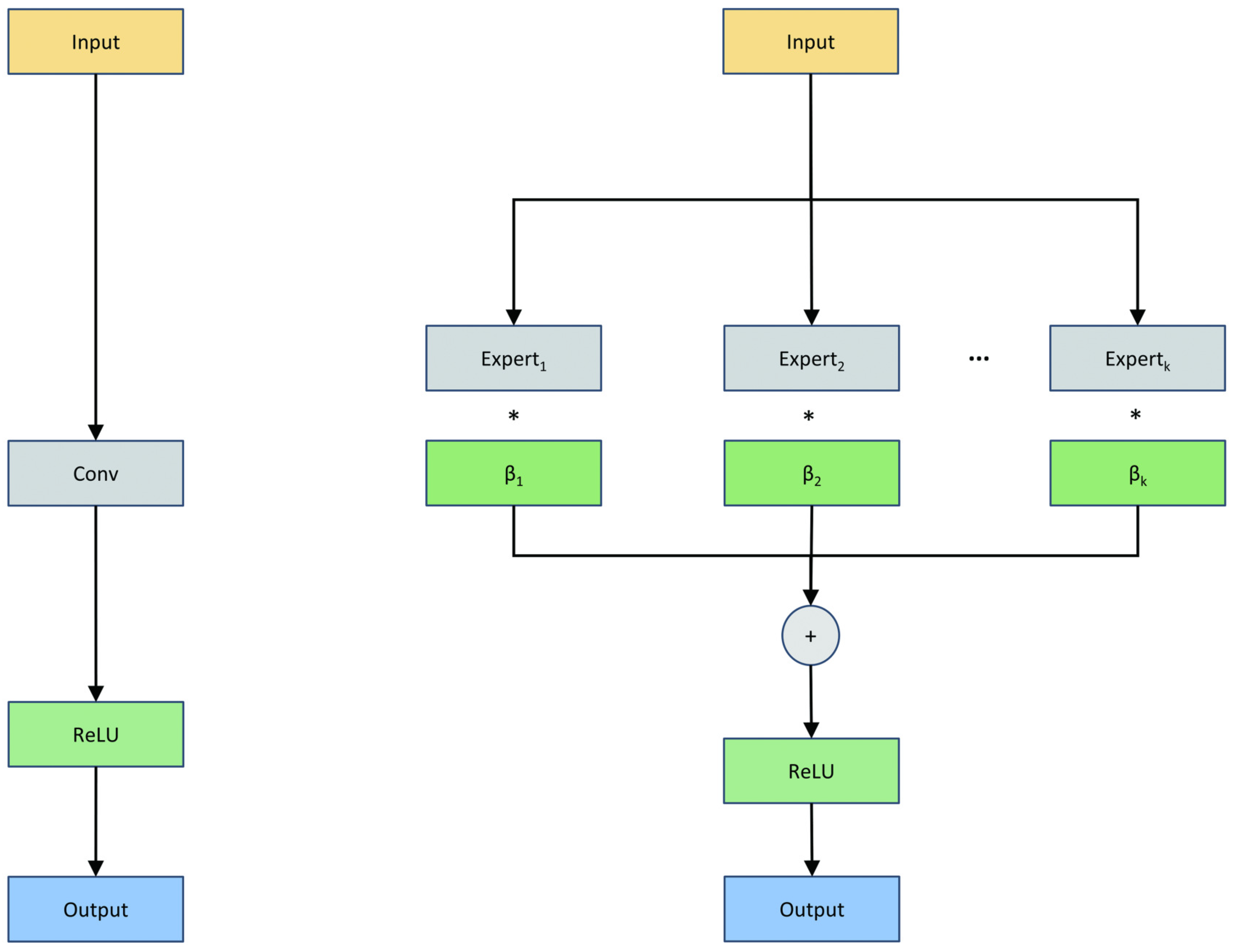
Inspired by this concept, we have incorporated Dynamic Convolution into our Ghost Module to increase the number of Params while keeping FLOPs low. Dynamic convolution selects and combines different convolutional kernels, known as “experts”, to process input data adaptively. This method serves as an extension of standard convolution, allowing the network to adjust its Params based on the specific input. By integrating Dynamic Convolution into the Ghost Module, we have developed our GND Bottleneck, which combines the efficiency of the Ghost Module with the adaptability of Dynamic Convolution to enhance feature representation.

In our implementation, Dynamic Convolution consists of K experts (with $K=4$ in this study), labeled from expert 1 to expert K. The principle is illustrated in Figure 7. The operation of Dynamic Convolution can be expressed as follows:

$${\mathrm{Expert}}_{\mathrm{final}}=\sum _{i=1}^K{\beta }_i·{\mathrm{Expert}}_i,$$

(4)

where ${\mathrm{Expert}}_i$ represents the i-th expert kernel, ${\beta }_i$ is the attention weight associated with the i-th expert, and ${\mathrm{Expert}}_{\mathrm{final}}$ is the resulting convolution kernel. These weights $\beta =[{\beta }_1,{\beta }_2,\dots ,{\beta }_K]$ serve as a set of attention coefficients that dynamically adjust the contribution of each expert kernel.

The weights $\beta$ are computed using the Squeeze-and-Excitation (SE) mechanism [28]. The input feature map first undergoes global average pooling to aggregate spatial information, followed by two fully connected layers with a ReLU activation in between and a softmax function at the end to normalize the attention weights. This process ensures that the selection of experts is input-dependent and contributes to improved adaptability.

Based on the insights of Han et al. [27], we analyze the calculation formulas for the parameter ratio of convolutional layers, as shown in Equation (5), and the FLOPs ratio required for convolution operations, as shown in Equation (6) (where M denotes the hyperparameter representing additional feature dimensions introduced in the intermediate layer, C represents the number of channels, and K is the kernel size). From this analysis, we understand that the parameter ratio depends on M and the kernel size K. When the FLOPs ratio for convolution operations approaches 1 and the spatial dimensions $H^{\prime }$ and $W^{\prime }$ are relatively large, the computational load can be almost negligible.

The parameter ratio of the convolution is

$$\begin{array}{cc}{R}_{\mathrm{param}}\hfill & ={\displaystyle \frac{C_{\mathrm{in}}^2+C_{\mathrm{in}}M+M{C}_{\mathrm{out}}{C}_{\mathrm{in}}{K}^2}{C_{\mathrm{out}}{C}_{\mathrm{in}}KK}}\hfill \\ \hfill & ={\displaystyle \frac{C_{\mathrm{in}}}{C_{\mathrm{out}}{K}^2}}+{\displaystyle \frac{M}{C_{\mathrm{out}}{K}^2}}+M\hfill \\ \hfill & \approx {\displaystyle \frac{1}{K^2}}+M.(M\ll C_{\mathrm{out}}{K}^2,C_{\mathrm{in}}\approx C_{\mathrm{out}})\hfill \end{array}$$

(5)

The FLOPs ratio is

$$\begin{array}{cc}{R}_{\mathrm{flops}}\hfill & ={\displaystyle \frac{C_{\mathrm{in}}^2+C_{\mathrm{in}}M+M{C}_{\mathrm{out}}{C}_{\mathrm{in}}{K}^2+H^{\prime }{W}^{\prime }{C}_{\mathrm{out}}{C}_{\mathrm{in}}{K}^2}{H^{\prime }{W}^{\prime }{C}_{\mathrm{out}}{C}_{\mathrm{in}}{K}^2}}\hfill \\ \hfill & ={\displaystyle \frac{C_{\mathrm{in}}}{H^{\prime }{W}^{\prime }{C}_{\mathrm{out}}{K}^2}}+{\displaystyle \frac{M}{H^{\prime }{W}^{\prime }{C}_{\mathrm{out}}{K}^2}}+{\displaystyle \frac{M}{H^{\prime }{W}^{\prime }}}+1\hfill \\ \hfill & \approx 1(1<M<H^{\prime }{W}^{\prime },C_{\mathrm{in}}\approx C_{\mathrm{out}})\hfill \end{array}$$

(6)

By integrating Dynamic Convolution into the Ghost Convolution, our model can adapt to features of varying scales while maintaining low FLOPs. This approach enhances the model’s expressiveness and generalization capability, ultimately improving its performance in detecting and classifying “Sunshine Rose” grapes.

2.3.3. Dual Convolution

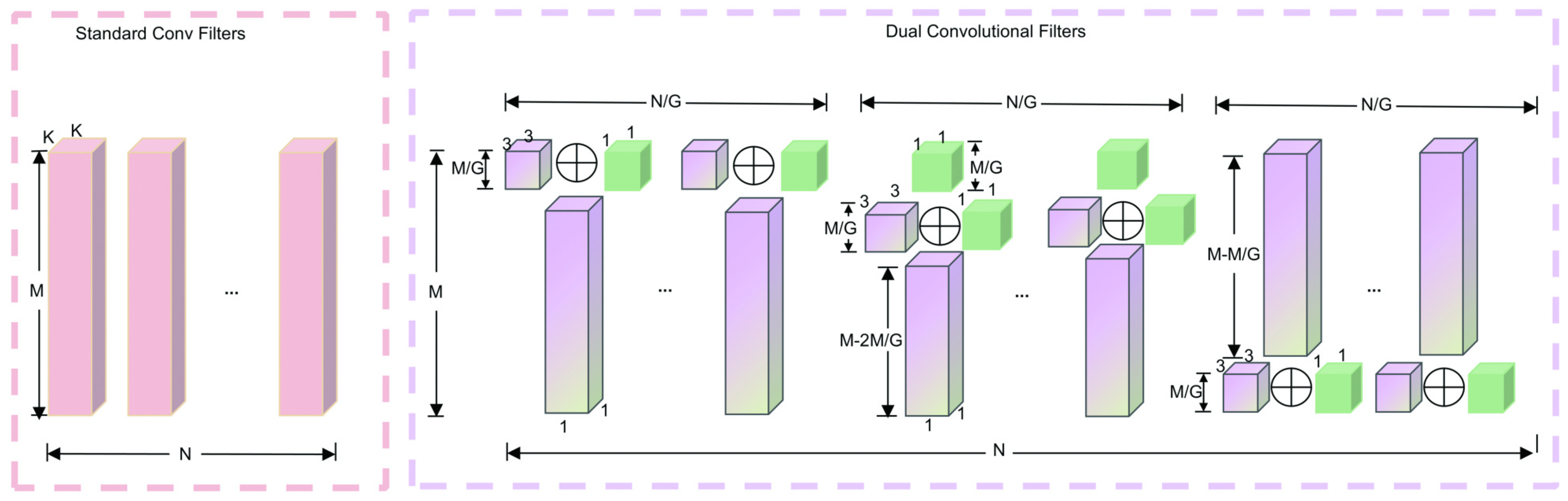
In our research, we replaced all standard convolution operations in YOLOv8 with DualConv, an approach that combines the strengths of GroupConv and HetConv.

GroupConv, known as “Aggregated Residual Transformations for Deep Neural Networks”, treats the convolution kernel as a three-dimensional filter, taking into account both channel and spatial dimensions. By decoupling inter-channel and spatial correlations, GroupConv enables more efficient mapping, resulting in improved performance. Specifically, the convolution kernel is divided into G groups, and the input feature map channels are also split into G corresponding groups. Each group of convolution filters processes its associated group of input channels independently, significantly reducing computational costs.

HetConv combines both $3\times 3$ and $1\times 1$ convolution kernels within a single convolution filter. These heterogeneous kernels are arranged alternately in a shifted pattern, with $3\times 3$ kernels placed discretely and interwoven with $1\times 1$ kernels, maximizing information processing flexibility within the same filter.

Our DualConv processes the input feature map through both $3\times 3$ and $1\times 1$ kernels simultaneously. Specifically, the operation can be expressed as

$$\mathbf{Y}=\sigma \left({\mathbf{W}}_{3\times 3}\ast \mathbf{X}\right)+\sigma \left({\mathbf{W}}_{1\times 1}\ast \mathbf{X}\right),$$

(7)

where $\mathbf{X}\in {\mathbb{R}}^{M\times H\times W}$ is the input feature map, and ${\mathbf{W}}_{3\times 3}\in {\mathbb{R}}^{(N/G)\times M\times 3\times 3}$ and ${\mathbf{W}}_{1\times 1}\in {\mathbb{R}}^{N\times M\times 1\times 1}$ are the $3\times 3$ GroupConv and $1\times 1$ kernels, respectively. Here, M represents the number of input channels, N is the number of convolution filters (i.e., output channels), and G denotes the group count for GroupConv. The activation function $\sigma (·)$ introduces nonlinearity.

The $3\times 3$ kernels focus on capturing spatial details in feature extraction, while the $1\times 1$ kernels facilitate inter-channel interaction and information fusion, all without substantially increasing the parameter count or computational load.

This enhanced DualConv architecture is depicted in Figure 8, where M, N, and G are further illustrated in relation to the kernel configuration and feature map structure.

3. Results

3.1. Environment and Parameter Settings

The training environment utilized in this study included an Ubuntu 12.3.0 operating system, supported by an Intel(R) Xeon(R) Platinum 8358 CPU, 512 GB of memory, and an NVIDIA A800 80G GPU for accelerated processing. The programming environment was set up with Python 3.9.19, PyTorch 2.2.1, and CUDA 12.1 for model development. For inference experiments, we used a separate platform with an Intel i7-12700 CPU. All training and inference procedures were implemented in PyTorch, without using any pre-trained models.

To ensure the robustness and reproducibility of our results, we maintained the initial values of all weights across all experiments. The hyperparameters were consistently maintained, as detailed in

Table 1. Training hyperparameters.

Image Resolution	Epochs	Batch	Batch	Lr	Optimizer
640 × 640	600	64	8	0.01	SGD

, where “Lr” represents the learning rate. The use of a fixed seed ensures consistent initial weights, thereby guaranteeing reproducibility. Model optimization was performed using Stochastic Gradient Descent (SGD), with a training limit set at 600 epochs. However, thanks to improvements in our model design, convergence was generally achieved within 200 epochs. To further optimize resource usage, an early stopping mechanism was implemented, which halted training if the mAP fluctuation remained below 0.1% for 50 consecutive epochs.

3.2. Evaluation Indicators

Precision (P) is defined as the proportion of correctly detected objects out of all detected objects, while Recall (R) represents the proportion of correctly detected objects out of all actual objects. The Average Precision (AP) is calculated as the integral of $P\left(R\right)$ over R, multiplied by 100%. The mean Average Precision (mAP) is the average of AP across all classes.

The formulas are as follows:

$$\mathrm{Precision}={\displaystyle \frac{\mathrm{TP}}{\mathrm{TP}+\mathrm{FP}}}\times 100\%$$

(8)

$$\mathrm{Recall}={\displaystyle \frac{\mathrm{TP}}{\mathrm{TP}+\mathrm{FN}}}\times 100\%$$

(9)

$$\mathrm{AP}=\int P\left(R\right)dR\times 100\%$$

(10)

$$\mathrm{mAP}={\displaystyle \frac{1}{m}}\sum _{i=1}^m\mathrm{AP}\left(i\right)$$

(11)

where TP is the number of true positives, FP is the number of false positives, FN is the number of false negatives, m is the number of classes, and $\mathrm{AP}\left(i\right)$ is the Average Precision for the i-th class.

3.3. Ablation Experiments

We conducted comprehensive experiments on each module of our model using the test set from the Shine-Muscat-Complex dataset to evaluate the effectiveness of our Ghost Module, Dynamic Convolution, and Dual Convolution in detecting “Sunshine Rose” grapes.

Table 2. Comparison of module impacts on object detection performance.

Ghost Module	Dynamic Conv	Dual Conv	mAP@0.5	mAP@0.5:0.95	P	R	FLOPs (G)	Parameter (M)	Time (ms)
✕	✕	✕	0.812	0.576	0.834	0.762	8.2	3.01	116.3
√	✕	✕	0.817	0.574	0.805	0.758	5.9	2.09	97.5
√	√	✕	0.833	0.581	0.813	0.777	5.8	2.18	99.6
√	✕	√	0.819	0.581	0.785	0.8	5.4	1.86	95.5
✕	√	✕	0.829	0.602	0.775	0.814	7.2	4.4	119.3
✕	√	√	0.828	0.593	0.779	0.82	6.8	4.2	117.1
✕	✕	√	0.812	0.578	0.801	0.797	7.7	2.7	113.3
√	√	√	0.838	0.602	0.865	0.775	5.4	1.9	98.2

below illustrates the specific impact of each module on mAP, the number of Params, FLOPs, and processing time. The symbol “✕” indicates that the corresponding module was not applied, while “√” indicates that the module was included.

From Table 2, it is evident that the incorporation of the Ghost Module improved the mAP from 0.812 to 0.817, thereby maintaining and slightly enhancing the model’s performance. Notably, in comparison with YOLOv8n, the addition of the Ghost Module resulted in a 28% reduction in FLOPs and a 30.5% decrease in the number of Params.

Subsequent application of Dynamic Convolution led to a significant improvement in the model’s mAP. Although this change resulted in a 4.3% increase in Params, it did not lead to a substantial rise in FLOPs, which actually experienced a decrease. Replacing all standard convolutions with Dual Convolution had a minimal impact on the model’s mAP but played a crucial role in achieving lightweight characteristics for our model. The “Time” column in Table 2 indicates the inference time measured on a platform equipped with an Intel i7-12700 CPU. Importantly, the introduction of C2f-GND and Dual Convolution significantly reduced inference time by 18.1 ms compared with YOLOv8n, making our design better suited to meet the inference speed requirements of edge computing devices compared with YOLOv8.

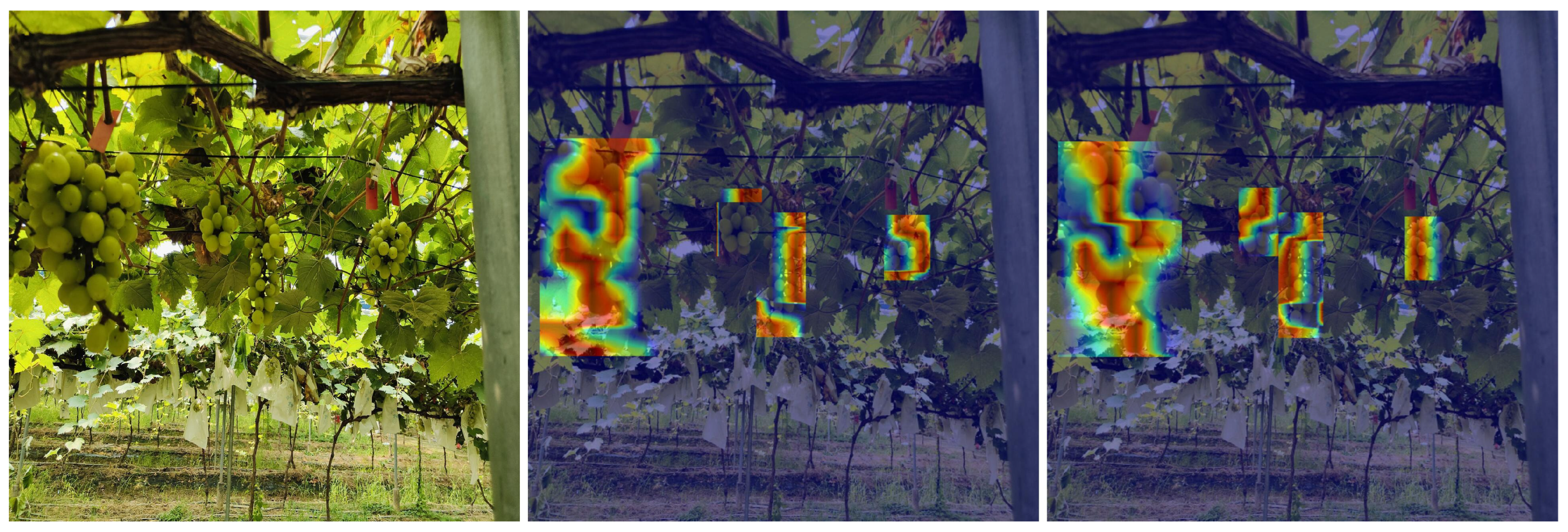
The replacement of the C2f module with our C2f-GND module resulted in notable improvements across mAP, Params, and FLOPs. As illustrated in the feature extraction heatmap comparison in Figure 9, the C2f-GND module substantially enhances the detection capabilities for small clusters of “Sunshine Rose” grapes. We hypothesize that this replacement allows the network to accommodate a more diverse range of data, thereby increasing its flexibility in addressing complex and varied datasets. Compared with the C2f module, the C2f-GND module can extract a broader array of features, enhancing generalization capabilities and improving the detection of small targets. Furthermore, while the original C2f module generated overly coarse bounding boxes, the C2f-GND module produces more accurate predictions by effectively extracting and fusing shallow positional feature information.

Although the integration of Dynamic Convolution in our model increased the Params from 3.01 million to 4.4 million, combining it with the Ghost Module reduced the Params to 2.18 million. Overall, the replacement of the C2f module with the C2f-GND module significantly facilitates target detection in complex scenes while addressing the lightweighting requirements essential for deploying the model on edge computing devices.

3.4. Comparative Experiments

3.4.1. Comparison with Other Deep Learning Models

Based on the analysis of our research objectives, this study prioritizes both accuracy and the deployment of lightweight models. To this end, we leveraged the high detection accuracy and real-time performance of the YOLO series for comparative experiments. This section details comprehensive training and inference experiments conducted on mainstream detection models, including YOLOv5n [29], YOLOv6n [30], YOLOv8n, YOLOv9t [31], and YOLOv10n [32], all under identical device conditions. The objective performance metrics are summarized in

Table 3. Comparison of detection performances of different detection networks.

Model	mAP@0.5	mAP@0.5:0.95	P	R	FLOPs (G)	Parameter (M)	Time (ms)
YOLOv5n	0.806	0.577	0.795	0.77	7.1	2.5	110
YOLOv6n	0.801	0.577	0.867	0.686	4.2	11.8	109
YOLOv8n	0.812	0.576	0.834	0.762	8.2	3.01	116.3
YOLOv9t	0.820	0.593	0.817	0.784	7.6	1.9	138
YOLOv10n	0.774	0.558	0.773	0.684	8.2	2.6	139
YOLOv11n	0.805	0.572	0.817	0.735	6.3	2.58	115
OURs	0.838	0.602	0.865	0.775	5.4	1.9	98.2

.

Upon evaluating various aspects of these models, we found that YOLOv5n and YOLOv6n exhibited the shortest inference times, each requiring only 110 ms. However, they did not excel in other performance metrics. YOLOv9t achieved the highest mAP0.5 at 0.820; nevertheless, its inference time significantly exceeded that of the other models, reaching 138 ms. Considering the specific requirements of our task and the need to balance mAP, Params, FLOPs, and inference time, we selected YOLOv8n as the baseline model. YOLOv8n offers the best balance between accuracy, size, and inference time, effectively meeting our mAP requirements for complex scenes while also satisfying the basic needs of resource-constrained edge computing devices.

Our improved model surpasses the baseline models across all evaluated metrics. Notably, our model’s mAP0.5 is 1.3% higher than that of YOLOv9t. Importantly, our model requires only 1.9 million Params and 5.4 GFLOPs. Furthermore, the inference time has been significantly reduced to just 98.2 ms, which is 10.4% faster than YOLOv5n. This achievement effectively demonstrates model lightweighting, making it suitable for a broad range of resource-limited edge computing devices.

In summary, following our improvements, YOLOv8n attains an exceptional inference speed of 98.2 ms, alongside a higher mAP. Most critically, our model’s Params and FLOPs have been reduced to 1.9 million and 5.4 GFLOPs, respectively. Consequently, our model is optimally designed for deployment on edge computing devices for the task of harvesting “Sunshine Rose” grapes.

3.4.2. Comparison with Lightweight C2f Improvement Methods

The C2f module is a vital component of YOLOv8, playing a significant role in enhancing detection performance. Through meticulously designed residual connections and convolutional stacking, the C2f module enables the model to effectively capture multi-scale and multi-channel feature information, thereby reducing computational load and accelerating inference speed.

In our study, we trained and evaluated several existing lightweight improvements to the C2f module, including C2f-CIB, C2f-DASI, C2f-CAA, C2f-Faster, C2f-Star, C2f-MS, and C2f-ODConv, to assess the efficacy of our proposed C2f-GND module. These lightweight methods are widely used to enhance computational efficiency and reduce model complexity, making them suitable for resource-constrained environments. The results of these experiments are summarized in

Table 4. Comparison of lightweight C2f improvement methods with the C2f-GND module.

Model	mAP@0.5	mAP@0.5:0.95	FLOPs (G)	Parameter (M)	Time (ms)
C2f-CIB	0.785	0.555	6.5	2.3	130
C2f-DASI	0.796	0.551	6.5	2.5	101
C2f-Faster	0.797	0.567	6.3	2.3	103
C2f-Star	0.806	0.572	7.0	2.5	110
C2f-MS	0.818	0.578	7.7	2.88	162
C2f-ODConv	0.814	0.586	5.7	3.07	116
C2f-GND (Ours)	0.833	0.581	5.8	2.18	99.6

.

A thorough analysis of the experimental outcomes revealed that the C2f-GND module consistently ranks either first or second across all evaluated metrics. Notably, our model incorporating the C2f-GND module demonstrates a significant advantage, achieving the highest mAP at IoU 0.5 (mAP0.5) among all models tested. Although the C2f-GND module slightly trails the optimal C2f-ODConv in terms of mAP0.5:0.95 and FLOPs, the differences are marginal, measuring only 0.005 and 0.1 G, respectively. Furthermore, the C2f-GND module significantly outperforms lightweight models in terms of Params and inference time, frequently surpassing the performance of alternative modules. This module effectively addresses the challenges associated with deploying models on edge devices, achieving an optimal balance between accuracy, computational load, and inference time.

In conclusion, following a comprehensive analysis of the experimental results alongside practical considerations, we identify the C2f-GND module as the most suitable choice for our task. It ensures high accuracy while maintaining a low computational load, parameter count, and inference time, making it ideal for the detection and classification of “Sunshine Rose” grapes.

3.4.3. Comparison with Two-Step Detection Methods

Two-step detection methods, such as Faster-RCNN, have historically been favored for their ability to handle complex detection and classification tasks by separating these processes into distinct stages. However, these methods are computationally expensive and often struggle with real-time performance, making them less suitable for edge computing applications.

To evaluate the effectiveness of our proposed model, we conducted a comparative analysis with Faster-RCNN. The results, summarized in

Table 5. Performance metrics comparison with Faster R-CNN on grapes detection.

Model	mAP@0.5	mAP@0.5:0.95	P	R	FLOPs (G)	Parameter (M)	Time (ms)
Faster-RCNN	0.782	0.594	0.583	0.821	447	42	1520
Ours	0.838	0.602	0.865	0.775	5.4	1.9	98.2

, demonstrate significant advantages of our lightweight approach.

From the results, our model achieves a higher mAP@0.5 and mAP@0.5:0.95, demonstrating superior detection performance and robustness across varying IoU thresholds. While the precision of our model significantly exceeds that of Faster-RCNN, indicating fewer false positives, the slightly lower recall suggests that Faster-RCNN is better at capturing hard-to-detect targets. However, this comes at the expense of computational efficiency, as our model drastically reduces FLOPs and parameters, making it more suitable for edge devices. Additionally, our inference time far outpaces Faster-RCNN’s 1520 ms, highlighting its practicality for real-time applications. Despite the slightly lower recall, our streamlined architecture offers an ideal balance between accuracy and efficiency, validating its potential for lightweight detection tasks in agricultural automation.

3.5. Detailed Experimental Results

To assess the effectiveness of our network improvements based on YOLOv8n for our research objectives, we conducted a comparative analysis of the model’s performance on the test set of the Shine-Muscat-Complex dataset, evaluating both objective and subjective metrics.

We employed precision (P), recall (R), inference time, Params, and FLOPs as our objective evaluation metrics. As illustrated in

Table 6. Performance metrics comparison with YOLOv8 on grapes detection.

Model	mAP@0.5 of Standard Grapes	mAP@0.5:0.95 of Standard Grapes	mAP@0.5 of Compromised Grapes	mAP@0.5:0.95 of Compromised Grapes	Precision	Recall	Time (ms)
YOLOv8n	0.937	0.664	0.688	0.488	0.83	0.762	116.3
Ours	0.940	0.666	0.737	0.537	0.86	0.775	98.2

, our model demonstrates significant enhancements in precision (P) and recall (R), with increases of 3.1 and 1.6 percentage points, respectively, compared with YOLOv8n. Notably, the mAP0.5 for the “Compromised grapes” category improved by 4.9 percentage points. Additionally, our model’s Params and FLOPs were reduced to 1.9 million and 5.4 GFLOPs, reflecting decreases of 36.8% and 34.1%, respectively, in comparison with YOLOv8n.

These results indicate that we have successfully enhanced detection performance while significantly decreasing inference time and FLOPs, thereby making our model more suitable for deployment on edge computing devices with limited computational resources.

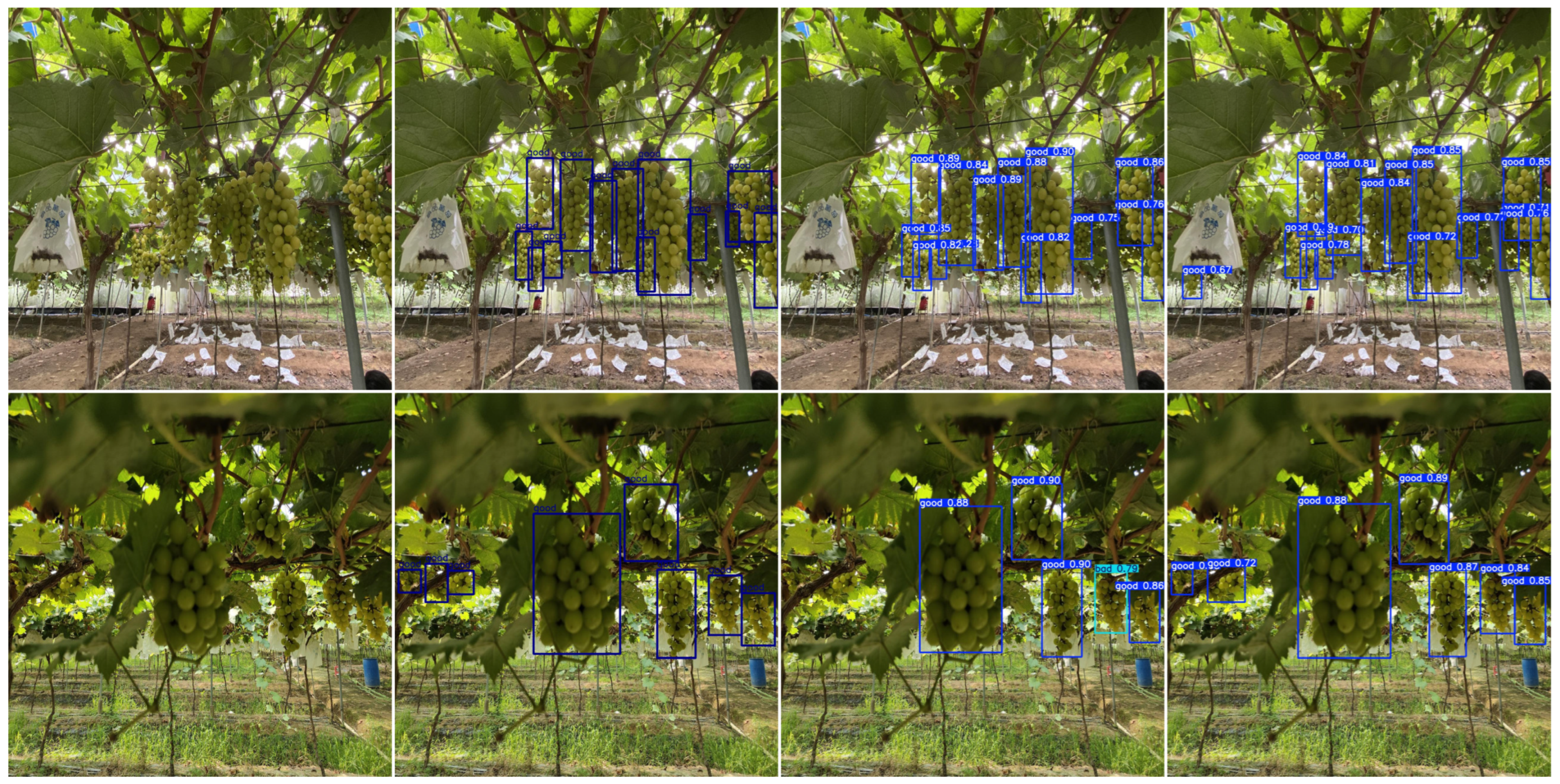
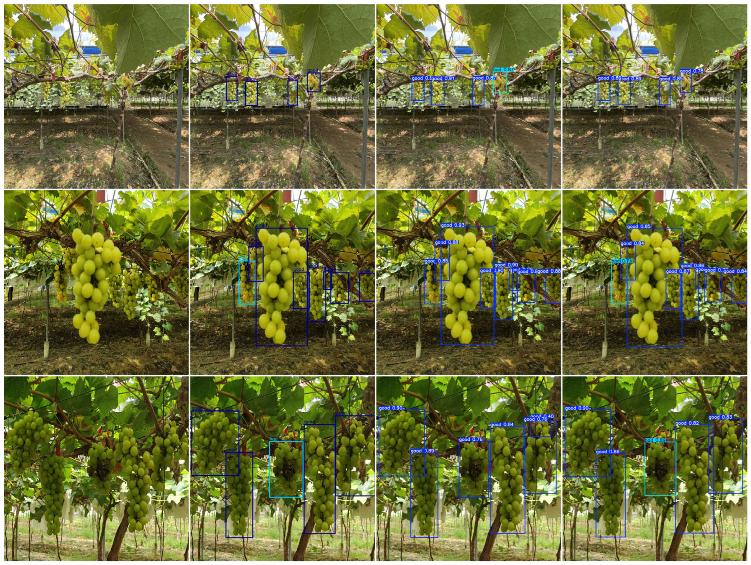
From a subjective standpoint, we evaluated the performance of our model in comparison with YOLOv8n by analyzing several sets of images.

Figure 10 illustrates the original test images, ground truth, and the detection results produced by both YOLOv8n and our model. The results clearly demonstrate that our model exhibits superior robustness in detecting small and overlapping targets when compared with YOLOv8n. Specifically, as shown in the third and fourth columns of Figure 10, YOLOv8n struggles to detect partially occluded and closely packed “Sunshine Rose” grapes, often missing or merging targets. In contrast, our model excels in these scenarios by effectively extracting multi-scale features through Dynamic Convolution. This enhancement allows our model to better capture the subtle characteristics of small and overlapping objects.

Furthermore, our model demonstrates significant adaptability to target detection under diverse lighting conditions. As evidenced in the second row of Figure 10, our model consistently identifies targets even in low-light and high-glare environments, where YOLOv8n frequently fails to perform reliably. By integrating improved feature extraction capabilities, our model mitigates the challenges posed by lighting variations and ensures accurate detection of overlapping and occluded targets.

The comparison underscores the practical advantages of our model over YOLOv8n in detecting “Sunshine Rose” grapes under complex conditions, confirming the effectiveness of our proposed architectural modifications.

Figure 11 presents the input images alongside the classification results from YOLOv8n and our model for several samples from the test set. A comparison of the classification results in the first row reveals that a cluster of “Sunshine Rose” grapes on the right is labeled as “Compromised Grapes” by YOLOv8n, while our model accurately classifies it as “Standard Grapes”. Upon magnifying the region, we observe that dark features near the cluster resemble the surface characteristics typically associated with “Compromised Grapes”. However, it is challenging to ascertain from this single image whether these dark areas represent genuine interference, such as withered leaves or grapevines.

To ensure the rigor of our subjective comparison, we analyzed images captured from different angles within the same scene. Our findings indicate that the dark pixels in this region do not correspond to the characteristics of “Compromised Grapes”, but rather are part of the background, specifically withered leaves. The detailed magnified view also shows that these dark pixels possess sharp edges, which are inconsistent with the rounded features characteristic of “Compromised Grapes”. Thus, we conclude that the dark pixels are more likely remnants of withered leaves in the background.

Overall, while our model demonstrates a better understanding of the subtle features of the detection targets, leading to improved classification performance, we acknowledge that its current evaluation is limited to the Shine-Muscat-Complex dataset. This dataset captures the unique characteristics of Shine Muscat grapes under complex orchard conditions. Although the dataset reflects diverse real-world scenarios, further validation of the proposed model on other datasets or crops will be necessary to evaluate its generalizability and practical applicability. Future work will focus on testing the model with different crop types and datasets to enhance its robustness and utility in diverse agricultural applications.

4. Discussion

This study proposes a lightweight YOLOv8-based model tailored for detecting and classifying “Sunshine Rose” grapes in complex orchard environments. The experimental results demonstrate significant improvements in mean Average Precision (mAP), computational efficiency, and inference speed, affirming the practical potential of the proposed model for real-world agricultural applications.

The proposed model offers several advantages. Its lightweight design enables deployment on edge devices, reducing reliance on high-performance computational hardware. This makes it suitable for agricultural applications in resource-constrained settings. The model’s ability to handle complex environmental challenges, such as occlusion, overlapping clusters, and uneven lighting, demonstrates its robustness. Furthermore, the integration of detection and classification tasks addresses practical agricultural needs, facilitating automated sorting of grape quality during harvesting. The integration of the Ghost Module and Dynamic Convolution into the YOLOv8 architecture effectively balances model complexity and performance. While the Ghost Module significantly reduces the number of parameters and floating-point operations (FLOPs), the Dynamic Convolution enhances adaptability to various environmental conditions. This combination ensures high accuracy and computational efficiency, meeting the practical demands of edge computing devices.

Despite these promising results, this study has some limitations that merit further discussion. First, the reliance on the Shine-Muscat-Complex dataset, specifically designed for “Sunshine Rose” grapes, may lead to overfitting to the particular conditions represented in the dataset, such as lighting, occlusion, and grape morphology. This raises challenges in generalizing the model to other grape varieties or crops with distinct characteristics. Strategies like transfer learning or incorporating more diverse training datasets that capture a wider range of environmental conditions and crop types could mitigate this limitation.

Second, while the model achieves robust performance in complex orchard environments, the classification accuracy for distinguishing “Standard Grapes” from “Compromised Grapes” still has room for improvement. Fine-tuning the model’s architecture or exploring more advanced feature extraction techniques could help address subtle differences between the two categories and further enhance its precision.

Third, adapting the model to other crops or agricultural scenarios poses additional challenges. Different fruits and vegetables may have varied morphological and environmental characteristics that require modifications to the network architecture or training strategies. Testing and fine-tuning the model on heterogeneous datasets will be essential to ensure scalability and adaptability.

In conclusion, this study contributes to precision agriculture by offering a robust and efficient model for automated grape detection and classification. However, addressing the discussed limitations will be critical for improving the model’s generalizability and adaptability. Future efforts should focus on validating the model across diverse agricultural environments and data types, including crops with varied morphological features, to promote broader applications of automated detection systems. By enhancing its scalability and robustness, this model has the potential to significantly improve operational efficiency and reduce labor demands in precision agriculture.

5. Conclusions

This study successfully developed a lightweight model based on the YOLOv8 architecture and constructed the Shine-Muscat-Complex dataset, specifically for detecting and classifying “Sunshine Rose” grapes in complex environments. By introducing DualConv and C2f-GND modules, our model significantly reduced the model’s parameter count, computational complexity, and inference time while maintaining high precision. Compared with YOLOv8n, our model achieved a 2.6% improvement in mAP, a 36.8% reduction in parameters, a 34.1% reduction in FLOPs, and a 15% decrease in inference time. These results not only demonstrate the effectiveness of the model but also provide new possibilities for deploying efficient object detection models on resource-constrained edge computing devices. However, this study has certain limitations. First, the dataset used in this study comes from only one crop species, and more data from various grape varieties and other crops need to be collected to test and verify the model. Second, when deploying and applying the model in practice, practical factors such as device compatibility and real-time performance must be considered. Therefore, in future research, we will further study the deployment on the edge to adapt to a broader range of application scenarios, as well as collect more data to extend the task to other grape varieties and more crops.