Article

Evaluation of Sugarcane Crop Growth Monitoring Using Vegetation Indices Derived from RGB-Based UAV Images and Machine Learning Models

by
P. P. Ruwanpathirana
1,2,*,
Kazuhito Sakai
1,3,*,
G. Y. Jayasinghe
2,
Tamotsu Nakandakari
1,3,
Kozue Yuge
1,4,
W. M. C. J. Wijekoon
5,
A. C. P. Priyankara
6,
M. D. S. Samaraweera
2 and
P. L. A. Madushanka
2
1
United Graduate School of Agricultural Sciences, Kagoshima University, 1-21-24 Korimoto, Kagoshima 890-0065, Japan
2
Department of Agricultural Engineering, Faculty of Agriculture, University of Ruhuna, Kamburupitiya 81100, Sri Lanka
3
Faculty of Agriculture, University of the Ryukyus, 1 Senbaru, Nishihara-cho, Okinawa 903-0213, Japan
4
Faculty of Agriculture, Saga University, 1 Honjo-machi, Saga 840-8502, Japan
5
Department of Soil Science, Faculty of Agriculture, University of Ruhuna, Kamburupitiya 81100, Sri Lanka
6
Computer Science, Faculty of Agriculture, University of Ruhuna, Kamburupitiya 81100, Sri Lanka
*
Authors to whom correspondence should be addressed.
Agronomy 2024, 14(9), 2059; https://doi.org/10.3390/agronomy14092059
Submission received: 8 August 2024 / Revised: 1 September 2024 / Accepted: 6 September 2024 / Published: 9 September 2024
(This article belongs to the Section Precision and Digital Agriculture)

Abstract

:
Crop monitoring with unmanned aerial vehicles (UAVs) has the potential to reduce field monitoring costs while increasing monitoring frequency and improving efficiency. However, the utilization of RGB-based UAV imagery for crop-specific monitoring, especially for sugarcane, remains limited. This work proposes a UAV platform with an RGB camera as a low-cost solution to monitor sugarcane fields, complementing the commonly used multi-spectral methods. This new approach optimizes the RGB vegetation indices for accurate prediction of sugarcane growth, providing many improvements in scalable crop-management methods. The images were captured by a DJI Mavic Pro drone. Four RGB vegetation indices (VIs) (GLI, VARI, GRVI, and MGRVI) and the crop surface model plant height (CSM_PH) were derived from the images. The fractional vegetation cover (FVC) values were compared by image classification. Sugarcane plant height predictions were generated using two machine learning (ML) algorithms—multiple linear regression (MLR) and random forest (RF)—which were compared across five predictor combinations (CSM_PH and four VIs). At the early stage, all VIs showed significantly lower values than later stages (p < 0.05), indicating an initial slow progression of crop growth. MGRVI achieved a classification accuracy of over 94% across all growth phases, outperforming traditional indices. Based on the feature rankings, VARI was the least sensitive parameter, showing the lowest correlation (r < 0.5) and mutual information (MI < 0.4). The results showed that the RF and MLR models provided better predictions for plant height. The best estimation results were observed withthe combination of CSM_PH and GLI utilizing RF model (R2 = 0.90, RMSE = 0.37 m, MAE = 0.27 m, and AIC = 21.93). This study revealed that VIs and the CSM_PH derived from RGB images captured by UAVs could be useful in monitoring sugarcane growth to boost crop productivity.

1. Introduction

The increasing global population has led to a continuing rise in the demand for food [1]. The global population will increase to 9–11 billion by 2050 [2], and global food demand will rise by 59% to 98% [3]. To meet the world’s food demand in the future, farmers must increase agricultural productivity. Numerous obstacles, including the effects of climate change, depletion of soil and water resources, urbanization, and rising input costs, stand in the way [4]; consequently, all countries need to concentrate on improving crop production by addressing these constraints.
The world’s consumption of sugar has been rising gradually over the past 50 years, and it is one of the most significant commodities globally, helping to improve socioeconomic conditions in many countries [5]. Sri Lanka’s sugar requirements for 2019 were 608,304 Mt, of which 91.4% came from imports. Sri Lanka spends about LKR 35.71 × 10⁹ a year on sugar imports [6]. In 2016, the government decided to increase sugar production to become 100% self-sufficient by 2025 by raising local sugarcane production [7]. Eighty percent of global sugar is produced from sugarcane (Saccharum spp. hybrids), and the rest is produced from sugar beet [8]. As a semi-perennial crop, sugarcane has a growth cycle of 9–12 months [9,10]. Its four main growth stages are germination (1 month after planting), tillering (1–3 months after planting), grand growth (3–9 months after planting), and ripening (10–12 months after planting) [11]. The potential for the sugarcane sector to provide a variety of outputs, including electricity generation, is enormous. In addition, sugarcane is used to produce bioethanol and a few other small-scale goods such as cane wax, molasses, and bagasse [12]. By the end of 2019, the volume of sugarcane harvested in Sri Lanka was 600,130 Mt [6]. Because there is enough suitable land in Sri Lanka, together with a climate ideal for sugarcane growth, the country is well-positioned to increase sugarcane production [13]. As a result, farmers and investors are working to maximize resource utilization while expanding the scope of sugarcane cultivation [14].
Numerous obstacles have been noted, including a lack of water, inadequate crop establishment and management techniques, labor scarcity, pests and diseases, challenges in retrieving field data due to its vast scope, and managerial challenges in sugarcane farming [13]. Sugarcane yield could be raised by using effective crop growth monitoring and decision support systems [15]. Optimal productivity and output of sugarcane can be achieved by the assessment and adjustment of the crop growth phase [10] but the traditional methods of manually monitoring crop development are time- and cost-intensive, unreliable, and prone to significant inaccuracies [16].
Precision farming techniques tend to be innovative and have the potential to significantly conserve time, reduce costs, and enhance the reliability and accuracy of crop monitoring [17,18]. Because it could instantly acquire multi-temporal and spatial images of crop growth in the field, remote sensing is one of the most popular and significant methods for providing crop information, such as crop type, status, and yield [9,19,20]. The most popular remote-sensing platforms are ground-based, satellite-based, and unmanned aerial vehicle (UAV)-based [21]. Ground-based platforms are limited because they are unable to operate in tiny fields and run the risk of destroying plants while gathering field data [21]. Satellite-image-based systems can provide continuous temporal and geographical data using instruments like Landsat, SPOT 5, and QuickBird so they have become a prominent tool in various crop-monitoring applications globally [16,21,22]. Agricultural applications for which satellite-imagery systems have been used across the globe include crop monitoring, yield and bio-mass estimation, pest and disease observation, stress identification, agricultural practice decision-making (particularly in management practices), crop mapping, crop spraying, and weed monitoring [18,23,24]. However, satellite-image-based platforms have several drawbacks, including low spatial resolution, high cost, and limited photo availability [25,26,27]. Thus, unmanned aerial vehicles (UAVs) could be used as a tool for monitoring crop growth and management because they are more affordable and easier to use in most locations, and they have shown great promise as a tool in long-term crop monitoring [25,27,28]. Benefits include high efficiency, flexibility, ease of use, and great terrain adaptation [29], and UAVs are generally considered to be a versatile tool for remote sensing in agricultural applications [30].
UAV technology has great potential for small-scale farmers because drones are now reasonably priced and come with open software, and relevant methods have been developed by researchers [27]. The technology can also be applied to scientific research, particularly in hard-to-reach locations where continuing observation is required [31]. The monitoring of crop growth by UAVs is becoming increasingly common [32]. In recent years, researchers have concentrated on examining the potential of UAVs to offer data on crop health, stress, and disease conditions [33]. Using a UAV camera and image processing software, Bendig et al. [34] obtained color images and created a three-dimensional geometric model for analyzing water stress in citrus trees. UAVs have been used in monitoring the growth of a variety of crops, including soybean [35], maize [36,37], wheat [38,39], and sugarcane [14,40].
Vegetation indices (VIs), derived from the reflectance of specific spectral bands in UAV images can be used to quantify crop health and vigor due to their functional relationship between spatial data and crop characteristics [41]. The normalized difference vegetation index (NDVI) is the growth metric most often used in remote sensing for crop monitoring and evaluation [40,42]. The combined ratio of the red band (R) and near-infrared band (NIR) radiations is used to calculate the NDVI [40] but the high cost of the four-band color infrared cameras needed to obtain NIR makes this an expensive method [43]. Since RGB (red–green–blue) cameras are less expensive than NIR-based cameras, they may be a better option for acquiring spatial images, particularly when used on UAVs to diagnose conditions such as crop growth and field anomalies [44]. Recent research studies discovered that vegetation indices derived from RGB images can be used to evaluate crop growth and development [36,40,45,46]. In addition, VI maps enable the identification of crop growth and development by estimating fractional vegetation cover (FVC) and image classification [47].
Plant height is also a crucial parameter for evaluating crop growth and yield. Regular monitoring of plant height can enhance crop growth and development by enabling farmers to make correct decisions such as implementing gap fillings at early stages, optimizing fertilization, and adjusting irrigation schedules [38]. Plant height measured using photogrammetric techniques such as crop surface models (PH_CSMs) is considered valuable structural data obtained from UAV images that can be used to evaluate crop growth and development [48]. RGB and multi-spectral UAV images have been used to estimate crop height in sugarcane, and results have highlighted a strong correlation between UAV-determined plant height and ground truth plant height [49,50]; however, slight differences between these data sources due to field variations and environmental factors have also been reported [51,52]. To overcome these problems, some researchers have recommended the integration of crop structural data and spectral data using machine learning (ML) techniques. Lu et al. [52] demonstrated that the combination of VIs and canopy height data improved the machine model accuracy for the above-ground estimation of wheat. Li et al. [19] found that the fusion of spectral and structural details obtained from RGB-based UAVs, combined with ML techniques, could be used to estimate maize biomass. However, studies on plant height estimation using RGB image data and ML methods are relatively limited and need to be extensively investigated, particularly in sugarcane growth monitoring.
In this context, most of the previous investigations have been oriented toward multi-spectral and hyper-spectral imaging techniques, which are indeed very effective—though not very inexpensive—and readily available to most farmers and researchers across the world [44,47]. Nevertheless, RGB-based UAV imagery has been the subject of limited studies on vegetation growth monitoring, especially for crops like sugarcane. Earlier studies have established the suitability of different VIs to assess the general health of vegetation cover [53,54] but few studies have attempted to fine-tune them for crop-specific conditions. Moreover, the combination of machine learning models with UAV-derived VIs and crop height is relatively new, while there exist vast possibilities for increasing predictive ability and decision-making when managing crops. This new approach improves the use of spectral and structural data obtained from RGB-based UAVs for accurately predicting sugarcane growth, providing significant improvements in large-scale crop-management strategies. Therefore, this study evaluated the accuracy of crop growth monitoring with growth anomalies at different growth phases in sugarcane cultivation in Sri Lanka using vegetation indices derived from UAV-mounted RGB cameras and machine learning methods.

2. Materials and Methods
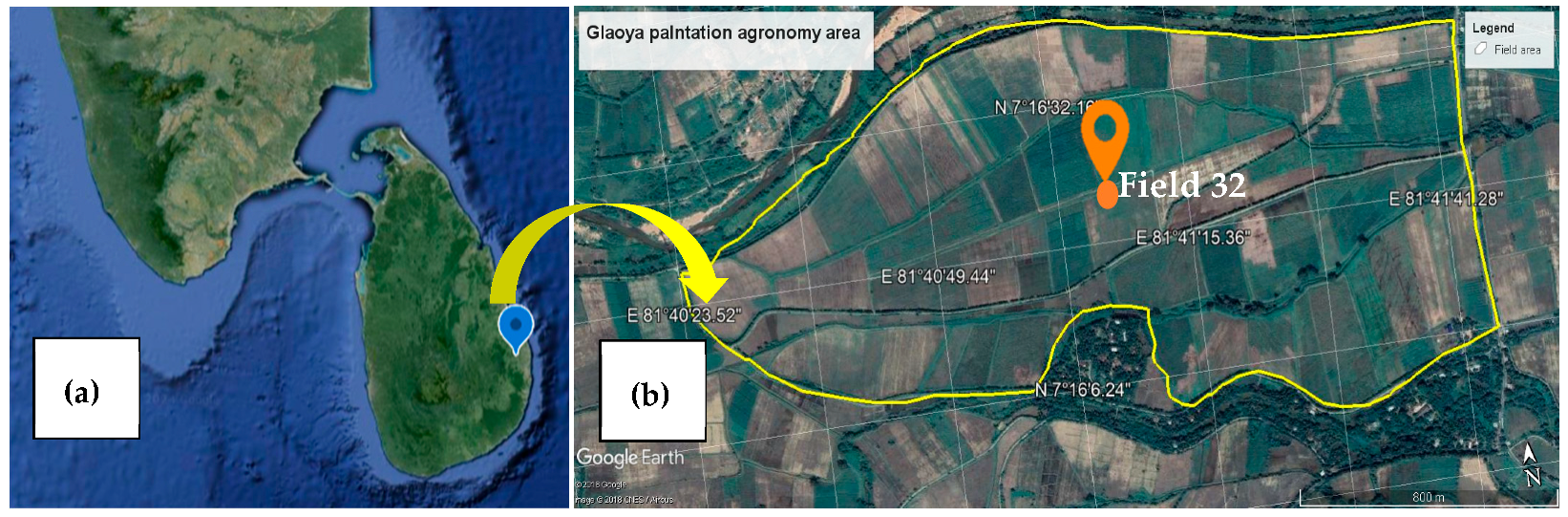
2.1. Study Area

This study was conducted on land owned by Galoya Plantation (Pvt.) Ltd. in Hingurana, ~14 km north of Ampara, in the eastern region of Sri Lanka (Figure 1). The sugarcane plantation covered 5200 ha (7°16′13.3″ N, 81°41′14.1″ E; 24 m above sea level). During the research period, the region experienced an average daily temperature of 29 °C, and the monthly rainfall ranged between 130 and 585 mm. The management aspects of this plantation were well-documented during the study period from September 2020 to March 2021 and this study draws on those data. An irrigated field (1 ha) with a well-developed commercial cultivar (SRI 128) was selected for the study area (Field 32 in Figure 1).

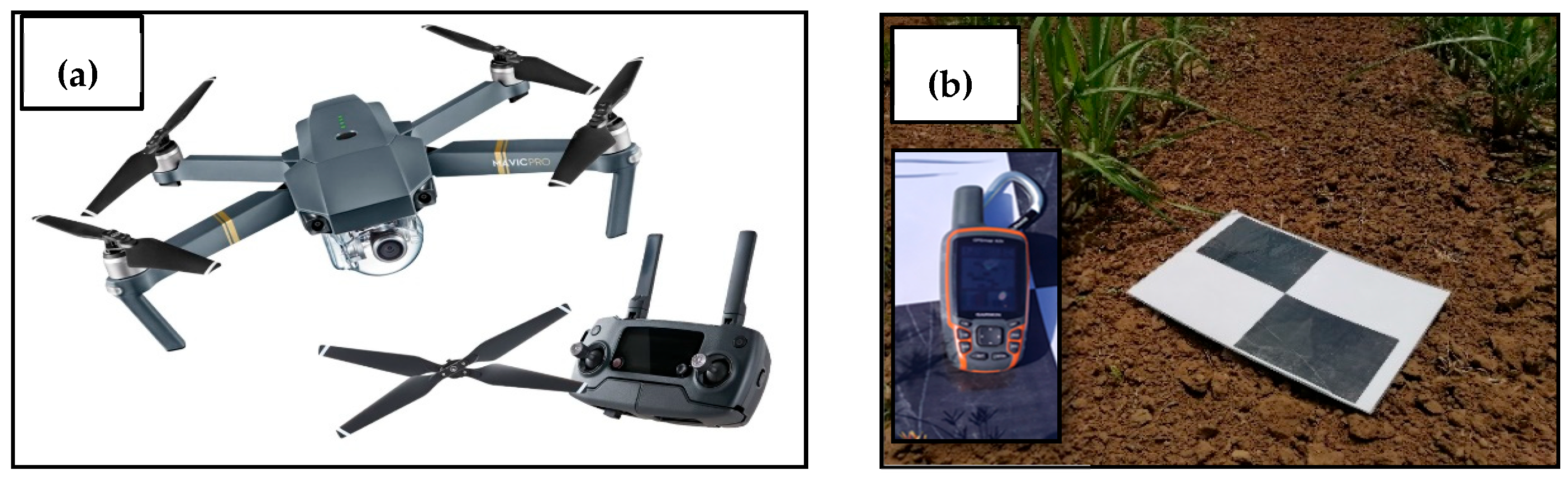
2.2. Description of the UAV

The RGB images for this study were acquired by using a DJI Mavic Pro drone (DJI Innovations Co., Ltd., Shenzhen, China) (Figure 2a). It consists of two main parts: a four-propeller aircraft and a remote controller that operates it. The aircraft has a maximum operating height of 500 m, a maximum travel distance of 13 km, and a maximum flying time of 27 min at a speed of 65 km/h. The drone is fitted with a DJI FC220 camera with an image size of 4000 × 3000 pixels, an inbuilt gimbal, a 3.722 mm focal length, and a 1/2.3-inch (6.17 mm × 4.55 mm) CMOS 12-megapixel sensor. The three visible spectral band sensors enable it to capture RGB images.

2.3. Flight Planning and Drone Image Acquisition

We captured aerial images of the 1-hectare field at four distinct stages of growth using the UAV system. The DroneDeploy application was used for mission planning on a smartphone. A previous study conducted by Ruwanpathirana et al. [55] suggested that the time of 10:00–12:00 was optimal for UAV operations in the chosen area to minimize the shadowing effects of images due to the sun’s direction. Therefore, aerial images were taken between 10:00 and 12:00 for all flights. Moreover, all UAV operations were conducted under excellent weather conditions including clear skies, consistent sunlight, and minimal wind (<10 m s−1). The images were captured at 50 m above the ground (1.5 cm/pixel), with 70% lateral and 75% frontal overlaps [55]. The camera was pointed toward the ground throughout every flight, and a total of 69 images were captured on each of the four flights. Table 1 shows the flight details at different growth phases. Before each UAV flight, 10 artificial markers (A4: 210 mm × 297 mm) were positioned on the field. These markers had to be visible in the pictures to be used as ground control points (GCPs) for georeferencing so that the photogrammetric model [56] could develop a digital surface model (DSM) using Arc GIS Pro 2.7 (Esri). Arc GIS Pro is a powerful geospatial tool, designed for creating, managing, analyzing, and visualizing geospatial data, including tasks like georeferencing, 3D modeling, and map production. The coordinates of the GCPs were recorded on a GNSS receiver (Garmin GPSMAP 62s) (Figure 2b). The steps involved in the UAV image acquisition procedure are outlined in Figure 3.

2.4. Ground Truth Data Collection

The stalk, nodes (where a leaf joins the stalk), and leaves typically make up a mature sugarcane plant. It can be challenging to conduct a manual field survey because of the plant structure. Bendig et al. [57] defined the height of a sugarcane plant as the distance from the top node to the ground. We measured plant heights in 20 plots (2 m × 2 m) of 10 plants using a meter ruler. The GPS coordinates were recorded at every sampling point. Any plant growth anomalies observed in the field were also recorded at this time.

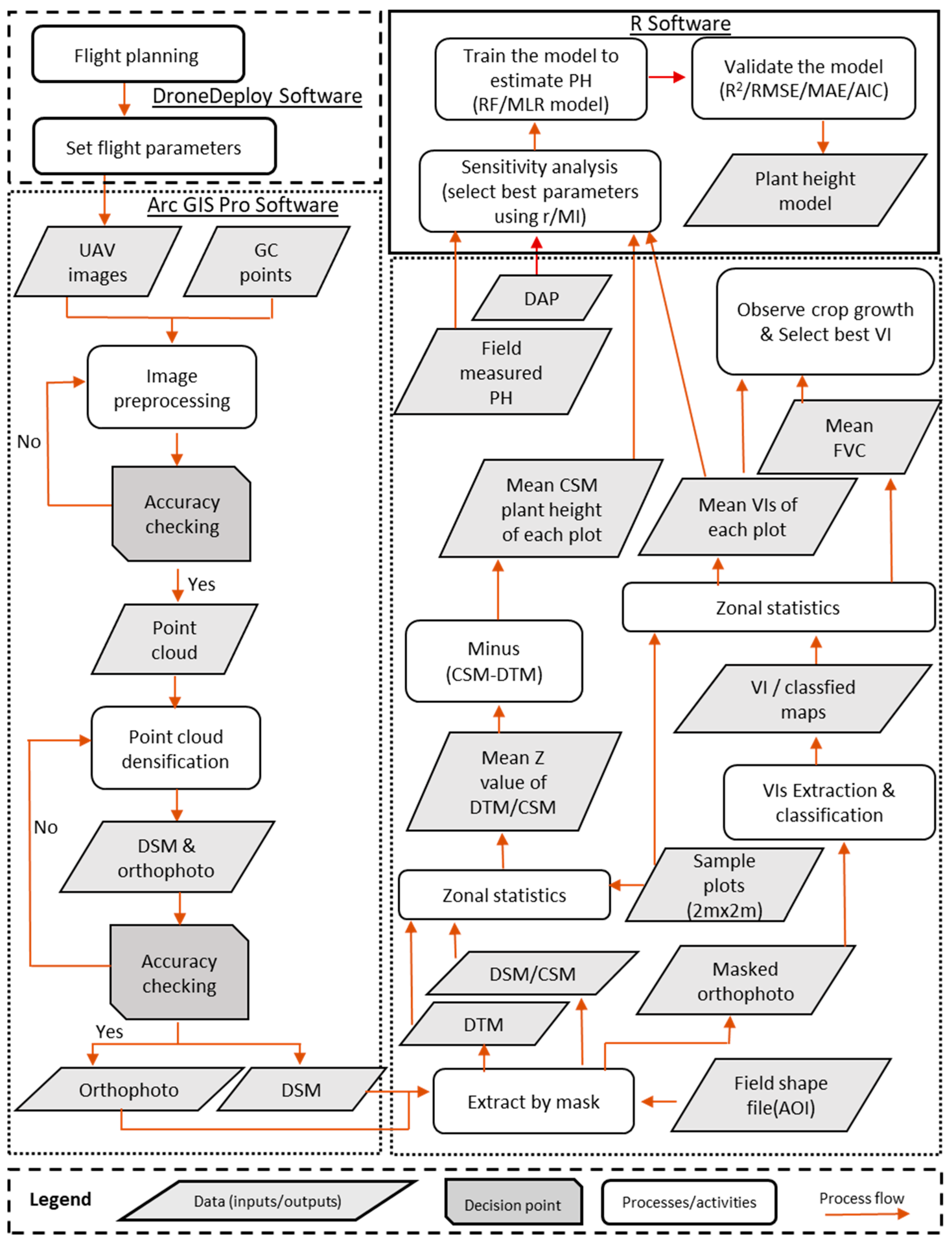
2.5. Feature Extraction from the UAV Image Data

The overall proposed conceptual framework for the image acquisition, data processing, and data analysis steps is shown in Figure 4. Following the captured images, the ortho-mosaicked images and DSMs were generated using Arc GIS Pro 2.7 (Esri) software during the image pre-processing step. Firstly, the imported images in Arc GIS Pro were georeferenced using UAV metadata and GCPs. Secondly, image alignment was performed by generating tie points to ensure the accuracy of overlapping images. Finally, detailed 3D models were created by point cloud densification to create orthophotos and DSMs.

2.5.1. UAV-Based Plant Height Generation from Crop Surface Models (CSM_PH)

Plant height derived from UAV images (CSM_PH) provides high-resolution, non-invasive, and accurate measurements across entire fields, enabling continuous and more accurate crop growth assessment by offering detailed spatial and temporal data on plant height variations [48]. The region of interest was established within the boundaries of the field map in Arc GIS Pro software. The digital surface models (DSM) characterizing the height of ground, vegetation, and man-made features were used to create the crop surface model (CSM) data. DSMs were imported into Arc GIS Pro, where they were used to create bare-ground models by removing vegetation and other man-made features, also known as digital terrain models (DTMs). Spatial filtering techniques were applied to remove high-elevation features representing vegetation and structures using the “Raster Calculator” tool in Arc GIS. Specifically, DSMs were transformed into Triangular Irregular Networks (TINs) to remove non-terrain features before converting back to raster format [58]. This procedure ensured that the DTMs accurately represented the bare ground, appropriate for terrain analysis. Equation (1) was used to calculate the mean plant heights at the selected sample locations [34]. The plant height values from crop surface models (CSM_PH) were obtained by subtracting the DTM from each CSM at each sampling plot (2 m × 2 m).
C S M _ P H = C S M D T M

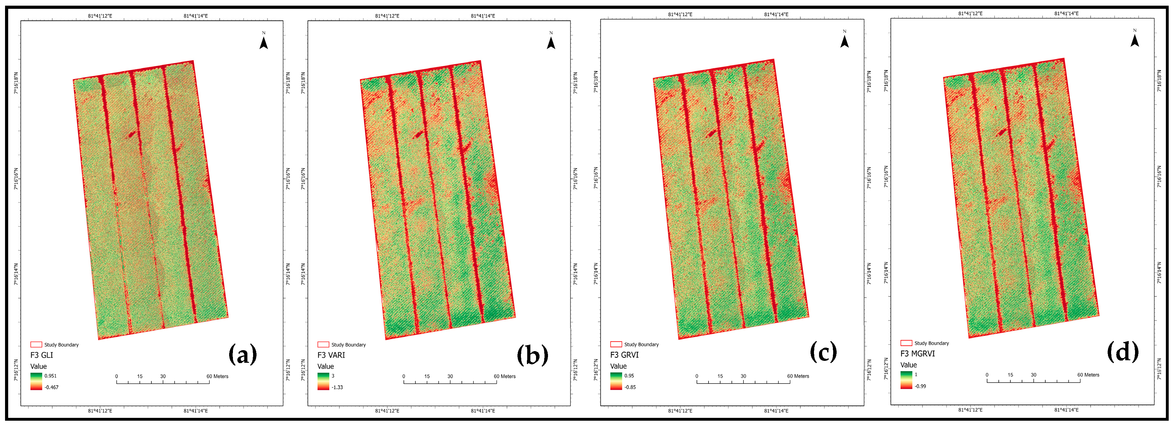
2.5.2. Computation of Vegetation Indices

Using the formulas listed in Table 2, the raster calculator in Arc GIS Pro computed four VIs based on the RGB spectral bands of the orthophotos. Green–red vegetation index (GRVI) is used as a phonology indicator to assess plant health by analyzing the ratio of green to red spectral bands [59]. In addition, GRVI can interpret ground cover and distinguish vegetation and soil areas based on its value [34]. The visible atmospherically resistant index (VARI) [46] utilizes the whole visible spectrum to estimate vegetation fraction with minimal sensitivity to atmospheric effects. The addition of blue wavelength reduces atmospheric effects and illumination differences. Green leaf index (GLI) is an effective indicator of vegetation greenness and plant health because of its high sensitivity to chlorophyll content. The high readings of GLI indicate healthy, green leaves and stems while low readings indicate soil or an absence of vegetation [60]. The modified green–red vegetation index (MGRVI) is designed to enhance the sensitivity of vegetation health assessments and provide field information by distinguishing between green and non-green areas [34].
These VIs were shown to provide superior findings for vegetation cover analysis in areas such as field healthiness, field gaps, low plant densities, and plant overlaps in maize and sugarcane [36]. Zonal statistics were used to obtain the mean values of the VIs per plot at each growth stage. The parametric statistical analysis was conducted using one-way ANOVA and least significant difference (LSD) tests to determine the significance of the mean VIs of each growth phase, at p < 0.05. All the analyses were conducted using R (v. 4.2.0).

2.5.3. Analysis of Crop Growth by Fractional Vegetation Cover (FVC) and Image Classification

Fractional vegetation cover (FVC) is an important phenotypic parameter that can be used to evaluate crop growth status and yield. FVC is typically measured by analyzing the fraction of the ground surface covered by vegetation [61]. In this study, the FVC of each VI map was computed utilizing threshold values of VIs and supervised classification (Equation (2)) [36]. The RGB mosaic images for each flight were identified as areas with or without vegetation by using the supervised classification approach (maximum likelihood classification), with 30 training sample points per class [62]. Using the kappa accuracy evaluation method, we used 100 stratified random sample points to test the picture categorization accuracy and computed FVC values for photos that were classified. To select the optimal VI, we calculated the classification accuracy values (Equation (3)) [36]. The crop growth rate was examined at the end of the crop growth cycle.
F V C % = N u m b e r   o f   p i x e l s   c l a s s i f i e d   a s   v e g e t a t i o n T o t a l   n u m b e r   o f   p i x e l s × 100
C l a s s s i f i c a t i o n   A c c u r a c y % = 100 ( V F O V F )
where VF is the FVC (%) of the vegetation index map; and OVF is the observed FVC (%) of the classified image.

2.6. Estimation of Plant Height Models for Crop Growth Monitoring by Machine Learning (ML)

2.6.1. Selection of Predictor Variables

In this study, the CSM_PH values were incorporated with vegetation indices to create a plant height prediction model. The selection of CSM_PH as a variable alongside VIs in the plant height prediction model is important because it improves the model accuracy by combining structural and physiological data. Thus, the predicted model could be used to identify crop anomalies and comprehensive crop assessment for site-specific crop-management strategies. In this study, field-measured plant height (Field_PH) served as the dependent variable, while the independent variables included CSM_PH and four vegetation indices—GLI, VARI, GRVI, and MGRVI—which were used during model development.
Feature selection is crucial in ML as it improves model performance by enhancing accuracy, reducing overfitting, and decreasing computational complexity. In this study, two common feature selection methods, Pearson’s correlation coefficient (r) and mutual information (MI), were utilized to select the most sensitive predictor variable to sugarcane plant height. Pearson’s correlation coefficient quantifies the linear relationship between dependent and independent variables, enabling the ranking of variable importance. Variables with the highest coefficients are considered the most significant predictors to be used in the prediction models [63,64]. MI measures both linear and non-linear relationships, helping to eliminate the least sensitive features. Higher MI values indicate stronger dependencies, while a value of zero suggests no dependency [65]. Therefore, these methods were performed to select the most influential predictor variables for plant height prediction.

2.6.2. Machine Learning Plant Height Prediction Models and Statistical Analysis

In this study, two widely used ML algorithms, namely Random Forest (RF) [66] and multiple linear regression models (MLR), were utilized to assess the performance of plant height estimation using the selected variables. RF is an ensemble learning technique that consists of many decision trees to improve the model accuracy and minimize overfitting. MLR is a low-complexity regression model that is used to predict dependent variables using multiple independent variables. We used these two ML methods in our study due to their high accuracy in regression modeling [67]. The models were performed in R (v. 4.2.0). The entire dataset, consisting of 80 observations, was used to develop a plant height prediction model by integrating data from each growth stage. The dataset was randomly divided into a calibration subset (75%) and a validation subset (25%). First, the regression models were calibrated using the calibration subset, and then, the calibrated model was applied to the validation subset. This process was repeated 500 times. Analysis of 500 results was used to select the best parameter combination. Based on the feature selection methods, feature combinations were created to identify the best model for predicting plant height using both crop structural data and spectral data. Each regression model was evaluated for the validation subset by analyzing the correlation between observed and predicted plant heights. The performance of both models was assessed by using the coefficient of determination (R2), root mean square error (RMSE), and mean absolute error (MAE) (Equations (4)–(6)) [64]:
R 2 = 1 i = 1 N ( y i y ^ i ) 2 i = 1 N ( y i y ¯ i ) 2
R M S E = 1 N i = 1 N y i y ^ i 2
M A E = 1 N i = 1 n y i y ^ i
where N is the total sample size; y i is the value of ith observation; y i ^ is the predicted value of ith observation; and y i ¯ is the mean measured value of ith observation.
Akaike’s information criterion (AIC) was used to compare the models [68] because it helps to identify the model that best explains the data within each set of model features [69]. We evaluated the models by calculating and comparing AIC values and the best-fitting model was selected with the minimum AIC (Equation (7)). R2 is not ideal for model selection with many variables because it may reduce model accuracy by overfitting data. Therefore, we used AIC to facilitate the selection of less complicated and more reliable models [70].
A I C = 2 k 2 ln ( L )
where k represents the number of estimated parameters in the model; and L denotes the maximum value of the likelihood function for the model.

3. Results

3.1. Visual Inspection of Crop Growth Monitoring at Different Growth Stages in Orthomosaic Images

Using visual observations based on the produced mosaicked images at different growth phases (Figure 5), we assessed the viability of crop monitoring. From the images, it is evident that plant growth increased rapidly from the tillering stage to the ripening stage. Differences in sugarcane tiller densities were identified at the tillering stage; the areas circled in black in Figure 5 had higher tiller densities. Canopy greenness was highest during the early grand growth stage (F2), and yellowing started in the later grand growth stage (F3). The early crop phases had more space between plots, but as the crop canopies grew over time, spacing decreased. Areas devoid of vegetation are visible as gaps in the plots, indicated by the yellow circles in Figure 5. Figure 6 shows a close-up photo of a barren area at the end of the crop cycle.

3.2. Vegetation Indices and Vegetation Cover Analysis at Different Growth Stages

Table 3 presents the mean VI values during each flight. The vegetation indices were not significantly different within each growth phase; however, VIs were significantly lower at the tillering stage than at the other three stages (p < 0.05). VI values were highest in the later grand growth stage (MGRVI = 0.138, GLI = 0.135, and GRVI = 0.072). All VIs except VARI peaked during the later grand growth stage and every VI decreased from then to the ripening stage. All VIs had the greatest values during the later grand growth stage (F3). The variety in vegetation patterns at that stage is shown in Figure 7.

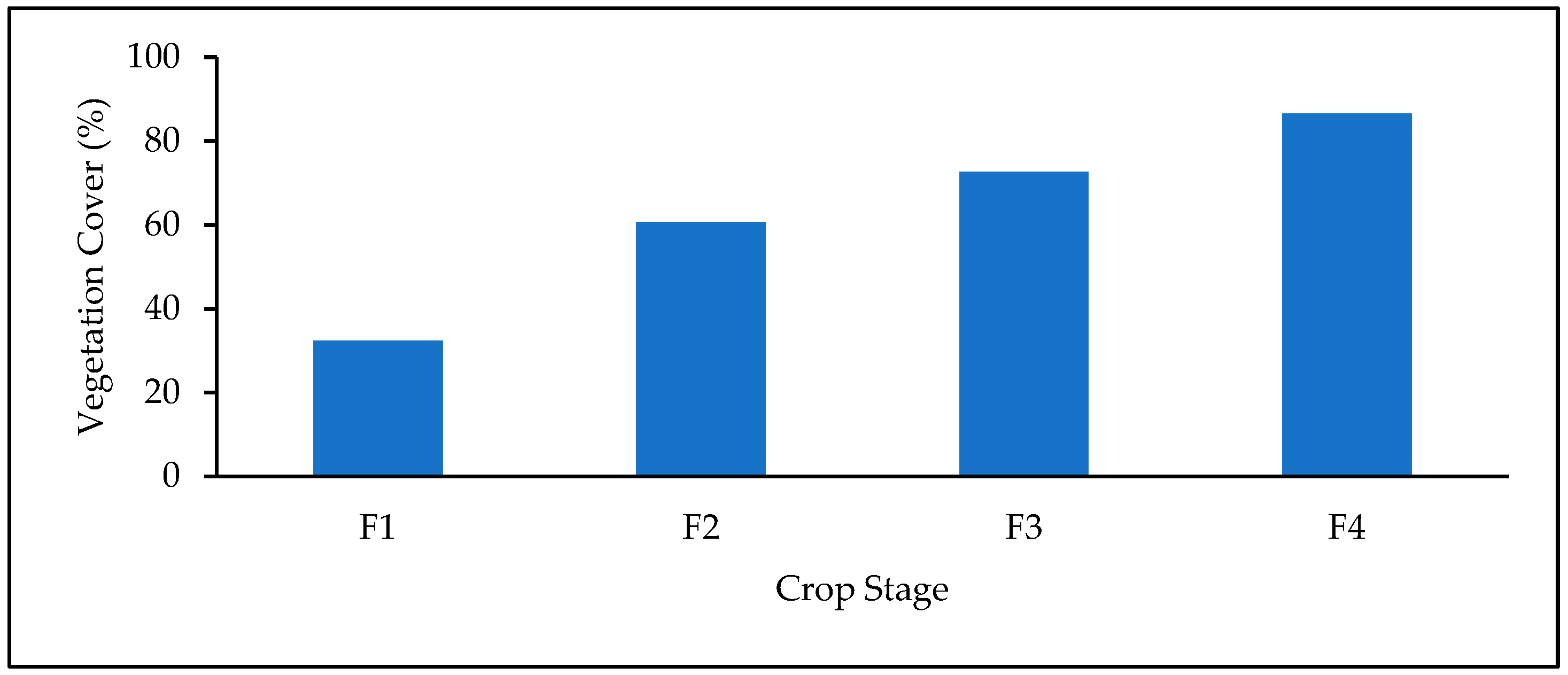
3.3. Image Classification and Fractional Vegetation Cover Analysis

The FVC values of all vegetation index maps were computed using supervised classification maps for the vegetation and non-vegetation classes for each flight. Based on these values, almost 90% of the field was covered by vegetation when it reached the ripening stage. Consequently, FVC values from the classification maps could be used to illustrate the development of crop growth from beginning to end (Figure 8). The highest incremental gain (28.33%) occurred from the tillering stage to the early grand growth stage.
The classification accuracies of the vegetation cover are shown in Table 4. Of the four VIs, MGRVI was deemed the best because of its categorization accuracy, which ranged from 94.58% to 99.09%. The accuracy values of all VIs decreased in the ripening stage but that of MGRVI decreased the least.

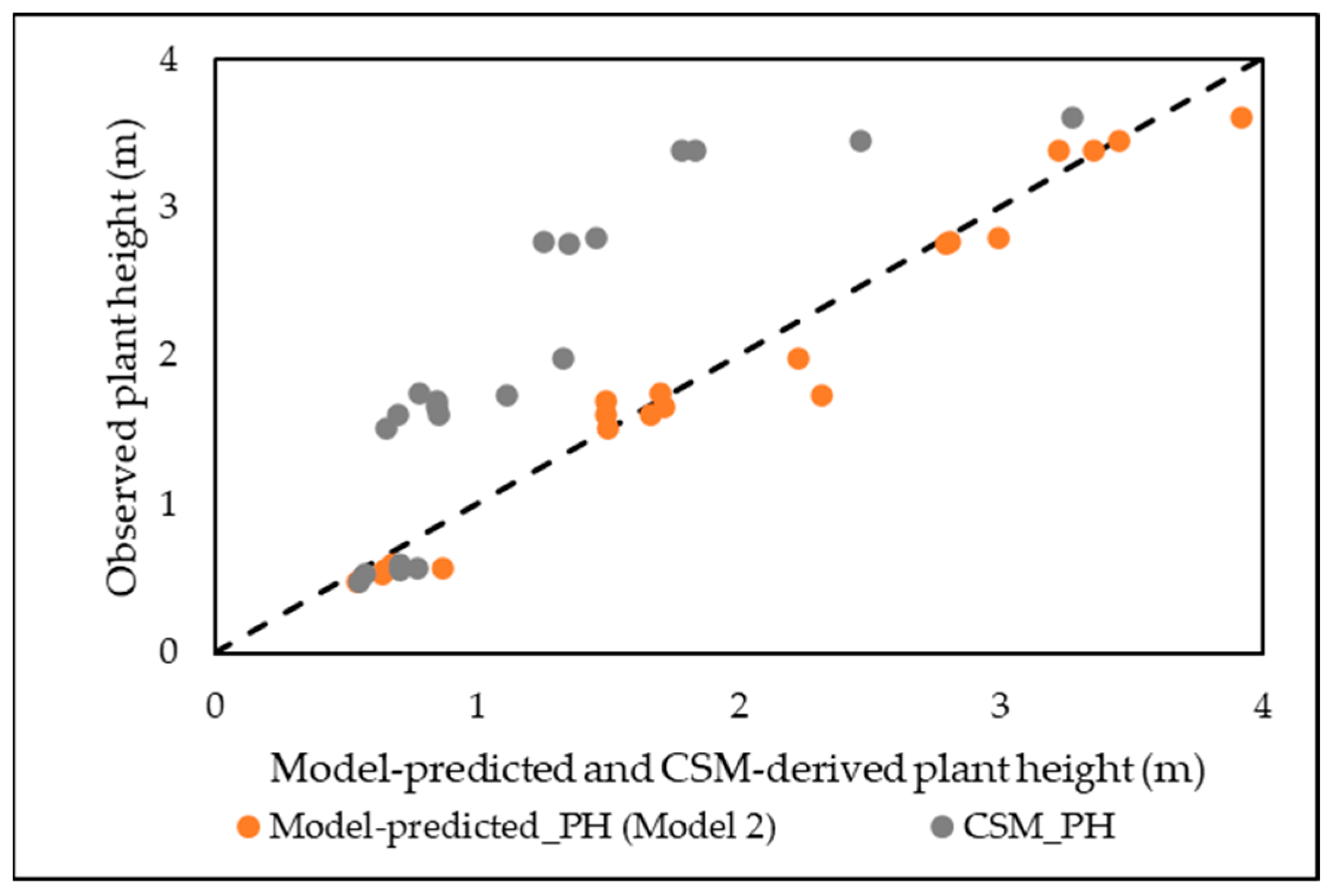
3.4. Plant Height Prediction from CSM

Table 5 shows the descriptive statistics for CSM_PH at the sampling sites. From tillering to ripening, the CSM mean values varied from 0.64 m to 2.29 m (SD < 0.59 m). CSM_PH increased with the growth stage, but variations were greater in the later phases. The CSM_PH showed slightly different values compared to Field_PH values.

3.4.1. Selection of Predictor Variables by Sensitivity Analysis

The feature importance of predictor variables for sugarcane plant height prediction models was ranked based on the results obtained from Pearson’s correlation and mutual information algorithms. Table 6 shows the variable ranking results based on their performance for both methods. The top-ranked features were highly sensitive in predicting plant height, while the lower-ranked variables showed less sensitivity. The most significant predictor variable for plant height was CSM_PH compared to others (r = 0.85 and MI = 0.706). In both methods, VARI showed the least contribution for plant height estimation (r = 0.466 and MI = 0.367). The top four ranked variables were selected to build plant height models (r > 0.50 and MI > 0.39).

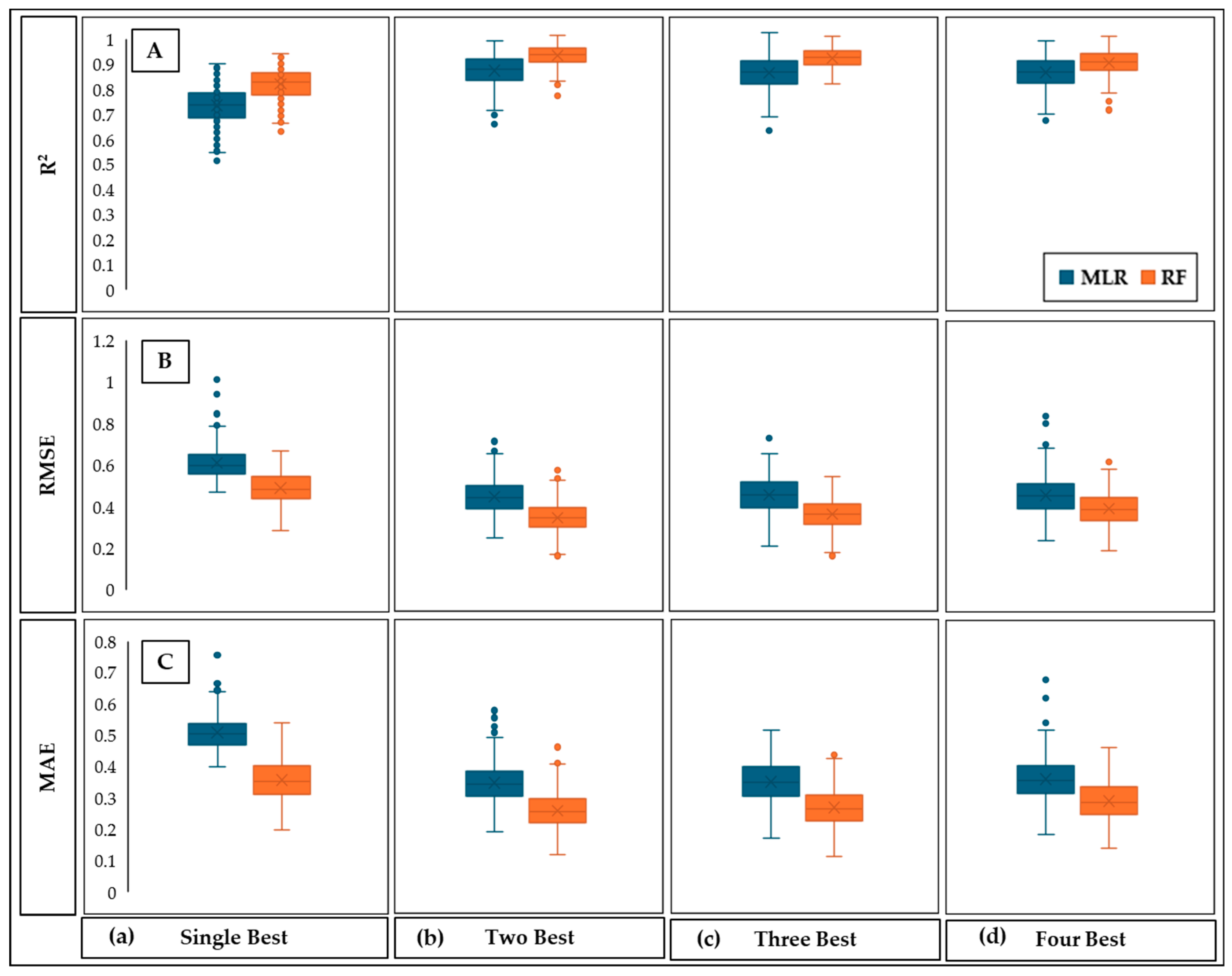
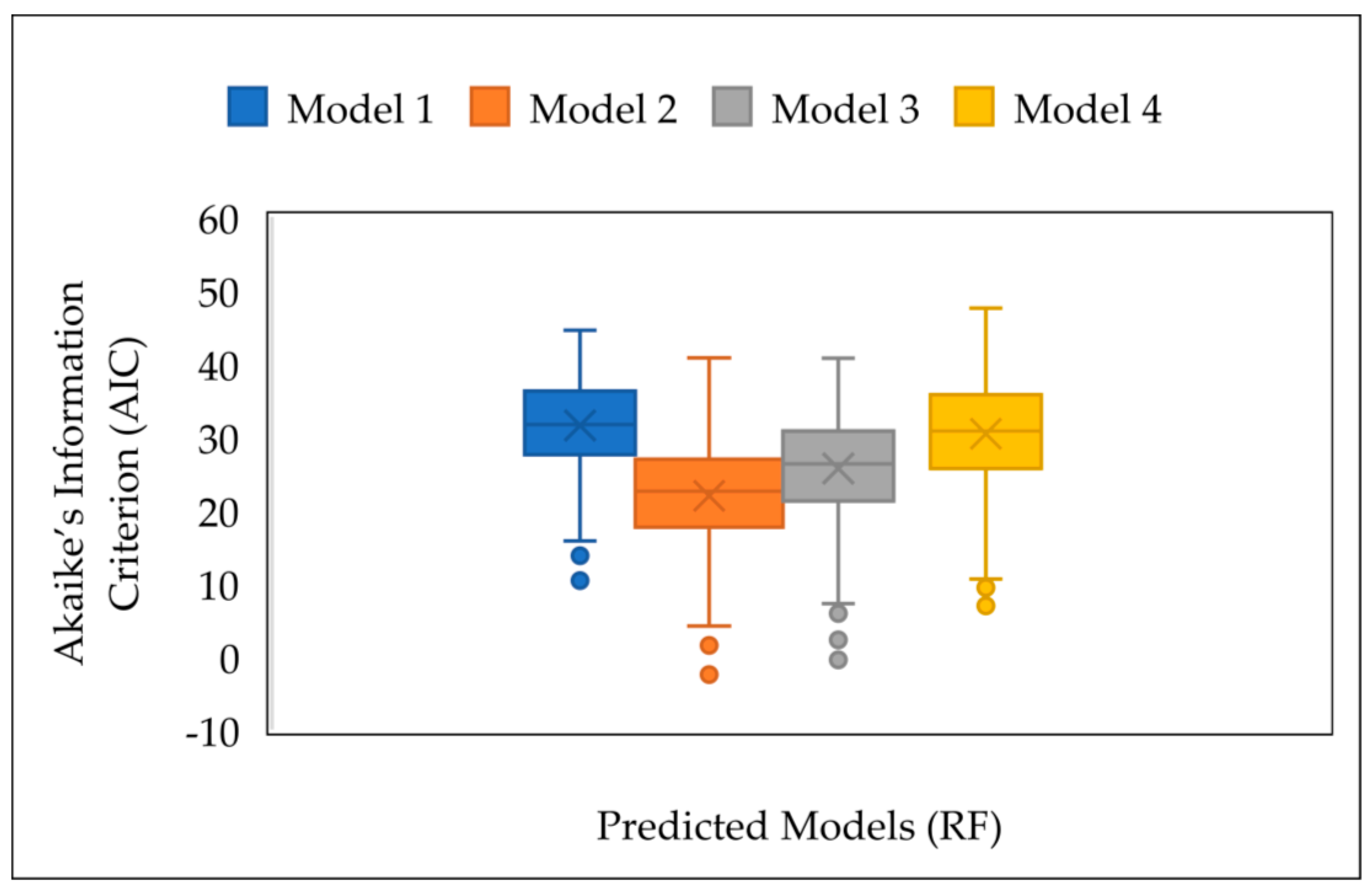
3.4.2. Prediction of Plant Height Using MLR and RF

Based on the feature selection method, four variable combinations were used to identify the best model for predicting plant height: (1) single best (CSM_PH); (2) two best (CSM_PH + GLI); (3) three best (CSM_PH + GLI + GRVI); and (4) four best (CSM_PH + GLI + GRVI + MGRVI). All models predicted plant height accurately based on the results of predicted models for both algorithms (Figure 9 and Table 7). Figure 9 shows a comparison of the model-predicted results of R-squared, RMSE, and MAE across 500 runs for both MLR and RF algorithms. The model using a single best variable (CSM_PH) exhibited lower performances than the other models for both methods, indicating the under-estimated values between CSM_PH and Field_PH. In addition, the fusion of CSM_PH and VIs data provided better results for both the MLR and RF models. In contrast, the RF algorithm outperformed the MLR method for predicting plant height (Figure 9).
The mean performance metrics indicated that plant height prediction models combining CSM_PH along with all VIs achieved the best performances for the RF algorithm (R2 > 0.85, RMSE < 0.42 m, and MAE < 0.31 m) (Table 7). Moreover, the model incorporating the two most predictive variables (CSM_PH + GLI) demonstrated the highest accuracy for both the MLR- (R2 = 0.84, RMSE = 0.46 m, and MAE = 0.35 m) and RF-plant height model (R2 = 0.90, RMSE = 0.37 m, and MAE = 0.27 m). The RF Model 3 also provided precise results but with slight differences from Model 2.
Increasing the number of variables in a prediction model can increase training time and reduce model performance. In addition, the number of parameters used for RF analysis is difficult because its inner structure is not visible. Therefore, we calculated the AIC values for the RF-predicted models to select the best-fit model for predicting plant height (Figure 10). AIC was highest for Model 1—which incorporates a single best variable (AIC = 31.55)—indicating that this model performed with the lowest accuracy compared to other models. Considering the lowest AIC, Model 2 (CSM_PH + GLI) was selected as the best-fit model for RF (AIC = 21.93). It is clearly shown that AIC values increase when increasing the number of predictor variables (Figure 10), indicating that the model’s accuracy may be reduced due to overfitting. Therefore, GLI provided the best performance when combined with UAV-derived plant height in sugarcane height estimation under RF-based models.
The scatter plot comparison between plant height estimates from the RF model (two best) and observed field plant height is displayed in Figure 11. The correlation between UAV-derived plant height and field-measured plant height is also plotted in the same graph to show the effectiveness of the model’s prediction. The larger discrepancies between Field_PH and CSM_PH were highlighted by the underestimated plant height values in the UAV-derived data; however, these differences are noticeably decreased when using the RF model in combination with the CSM_PH and GLI variables. Thus, the RF model provides more accurate and reliable plant height predictions by integrating structural and spectral data from RGB-based UAV imagery.

4. Discussion

We first analyzed the crop growth status of a sugarcane field by visual interpretation of mosaicked images over time. Vegetation cover and soil areas could be easily visualized in the early stages of the crop cycle (up to 3 months after planting). Montibeller et al. [71] noted that UAV mosaic images could be used to visualize vegetation cover and exposed soil areas in sugarcane plots. The regions marked in black (F1 in Figure 5) had greater tiller densities and overlapping seedling rows, most likely because of inadequate management practices and environmental conditions such as rainfall, sunlight, and wind [63]. The orthomosaic images captured during early crop growth could be used to aid management in high-tiller-density areas, for example, by alerting a farmer to apply low dosages of fertilizer to those locations. Intra-field variations could be observed by using enlargements of the orthophotos (Figure 5). A large barren area due to inadequate seed cane germination was seen in the same region during F2, F3, and F4 flights. Sumesh et al. [49] used a drone to classify sugarcane fields based on RGB images, and barren fields were visualized using an orthophoto of the field. UAV technology is critical for making decisions to address this kind of issue and aids in the identification of such field anomalies in the early stages of cultivation. According to Du and Noguchi [72], the crop growth status of wheat could be visually observed at different growth stages using orthomosaic images derived from UAV images. As a result, by visualizing the mosaicked images, the UAV approach could be used to monitor crop growth status.
RGB-based VI maps were created to analyze the growth of sugarcane in different growth stages. The results showed that no significant differences in vegetation indices were observed within each growth phase, suggesting that all indices provided similar plant growth information and may be equally effective in crop monitoring for each stage. The tillering stage showed significantly lower VI values compared to other stages (p < 0.05), indicating the lower canopy development at the tillering stage compared to the vegetative and ripening stages. Moreover, the lack of significant differences in VIs at later growth stages may be attributed to crop maturity, which results in a denser canopy. The results revealed that the quantification of VIs provided detailed information for monitoring the progression of crop growth and development. The VARI map had a very high greenness value (a maximum of about three, Figure 7b) because VARI eliminates illumination differences. As a result, the VARI results could not be easily used to validate the results based on visual observations or estimated values [73]. In contrast, the GLI, GRVI, and MGRVI maps all have maximum values close to one (Figure 7a,c,d), indicating that there were many leaves and stems in the field. With crop growth and development, all VI values increased from the tillering stage to their maximum in the later grand growth stage. All VIs decreased from the later grand growth stage to the ripening stage because crop canopy greenness begins to decrease during the later vegetative stages and to its lowest during the ripening stage. GLI values range from 0 (no chlorophyll content) to 1 (the highest chlorophyll content). The highest GLI value in our study was 0.135, suggesting a high chlorophyll content and that the GLI values increased from the tillering stage to the later grand growth stage [73]. VARI values were low at each stage and decreased after the early grand growth stage, indicating that atmospheric factors such as light were affected when estimating the proportion of vegetation [46]. The GRVI and MGRVI values were highest during F3, indicating peak plant phenology [34]. The GRVI values were lower at the start, indicating that there were more soil areas due to the low plant density. Sanches et al. [74] estimated sugarcane yield and obtained comparable results with a low GRVI value (−0.033) at the first stage. Fu et al. [39] reported that VIs can be used to detect the crop growth status of wheat at various crop stages. GLI, GRVI, and MGRVI maps could be used to distinguish plant growth and development in terms of plant height, vegetation cover, and the number of tillers or canes at different stages of growth because the images provide detailed information about crop growth status. The VI maps as well as the mosaicked images also identified field gaps, plant row overlaps, and abnormal plants. Field anomalies in the images were validated by field observations. Analyses of field management practices and anomalies using mosaicked pictures or VI maps may be beneficial in increasing total productivity by helping farmers make better decisions during the early stages of crop growth.
The computed FVC values showed the crop growth increment over time due to the increasing crop canopy from the tillering stage to the ripening stage. All the VI maps gave high accuracy (>90%) until the later grand growth stage, demonstrating the effectiveness of FVC in monitoring crop growth progression throughout the crop season. The highest growth increment (28.33%) was observed between tillering and early grand growth stages, indicating the rapid canopy expansion during key growth stages. According to the results, classification accuracy differed in all the selected VIs for all growth stages. Visible VI employs a combination of numerous visible light bands to provide details for image classification of vegetation and non-vegetation areas in a chosen field. The RGB bands used for the quantification of VI may affect the image classification results. Compared to the selected VIs for our study, MGRVI showed the best results (>94%) because of its ability of higher sensitivity to subtle variations in vegetation structure. Unlike other VIS, MGRVI utilizes a modified formula with squared values of red and green bands, which helps to distinguish vegetation and non-vegetation by adjusting the relative differences between green and red bands [75]. In addition, due to the higher sensitivity of MGRVI, it reduces soil background effects and increases the classification accuracy during later growth stages with dense canopy structures. Other VIs—GRVI, VARI, and GLI—showed lower accuracy results (<75%) at the ripening stage due to their lower sensitivity to the effects of soil background and variations in vegetation structure. Thus, MGRVI was selected as the best VI compared to others because it exhibits better classification results. Similarly, Felix et al. [76] suggested that MGRVI could be used effectively for vegetation cover analysis in aerial images with higher performances. Tumlisan [36] investigated six RGB-based VIs for detecting vegetation cover in maize and found that the best VIs had accuracy ranging from 91.45% to 99.16% at a 60 m flight height. Our results are even more accurate because we can readily distinguish between vegetation and non-vegetation areas in sugarcane crops, as in maize crops, because sugarcane plants are planted in specified rows with precise spacing.
Sugarcane plant height is an important indicator for assessing crop growth status, and it is directly related to yield [77]. Field-measured plant heights differed slightly from UAV-derived heights. These underestimates were higher in the later growth stages. This variation in plant height may be attributed to factors such as leaf angle orientation and canopy structure during the later growth stages [77]. Moreover, capturing the canopy of plants like maize is a challenge because of their distinctive canopy structure [52]. The plant heights were highly variable throughout the field according to the elevation maps. At the boundaries of the plots, plant heights were higher during F2, most likely because moisture availability is higher at the boundaries because of the irrigation setup. However, the elevation values in the DSM maps have been observed to change over through the crop growth cycle. This issue could be caused by the image processing step, which uses different brightness values for identical objects [78]. Another reason for plant height variation during the growth period would be environmental factors such as climatic conditions, water deficiencies, waterlogging, and soil type [36,79]. In a similar study, CSM heights varied significantly across sample plots [80].
Owing to the heterogeneity in CSM_PH, we used machine learning techniques to integrate the full dataset and create a plant height prediction model. In this study, we selected the most sensitive predictor variables for plant height prediction based on their relative importance, aiming to mitigate the reduction in model accuracy associated with using numerous variables. UAV-derived plant height (CSM_PH), which reflects the vertical structural characteristics of crop canopy, was shown to be the most significant parameter for plant height in the sensitivity analysis (r = 0.85 and MI = 0.706). In addition, all VIs showed relatively lower correlations for predicting plant height. Similarly, previous studies revealed a higher correlation between field-measured- and UAV-measured plant height compared to the spectral indices, which supported our results [19,52]. The CSM_PH was highly sensitive to plant height because it provides more details of crop structure and the growth status of the sugarcane canopy [19]. Nevertheless, GLI, GRVI, and MGRVI had the highest correlations (r > 0.5) with plant height because they are sensitive to changes in biomass and chlorophyll content. These indices serve as useful plant growth indicators since plants grow taller as their biomass and chlorophyll content increases. However, a moderate correlation was observed between individual VIs and plant height due to the large spectral variations. Aasen et al. [81] and Li et al. [19] reported that the accuracy of spectral data can be improved by combining different VIs with spectral data in model prediction. Finally, four variables (CSM_PH, GLI, GRVI, and MGRVI) with their best performance (r > 0.5 and MI > 0.39) were selected to use as a predictor input for model predictions. In a previous study, Ramos et al. [82] reported that they selected the top three ranked variables out of thirty-three VIs with higher correlations (r > 0.5) for yield prediction in maize.
The models predicted using CSM_PH and selected VIs showed that MLR and RF machine learning models provide better performance in plant height prediction. However, the accuracy was lowest when we used a single variable (CSM_PH; RMSE > 0.45 m, and MAE > 0.35 m). Underestimation and overestimation in UAV-measured plant height due to canopy overlaps at later stages and to environmental factors agreed with the findings of Ranđelović et al. [83]. Therefore, we compared the results of using combined canopy structure information (CSM_PH) and VIs as input data for model development, utilizing different input combinations to provide both structural and spectral information. The combination of CSM_PH and VIS demonstrated better results in plant height predictions for both ML methods. Lu et al. [52] suggested that the use of combined VIs and canopy height metric information improved the estimation of wheat above-ground biomass. Our results demonstrated that RF provided -higher accuracy compared to MLR in all predicting models. A previous study investigated by de Oliveira et al. [67] reported that RF models provided better results than MLR in predicting sugarcane plant height. The RF method proved to be the most suitable for interpreting the complex correlations between input parameters and target variables as it is not sensitive to overfitting [52].
Increasing the number of predictor variables can increase model complexity, prolong training time, and reduce model prediction performance [68]. To address this, we compared the models using AIC values in the RF models. The best-fitted model included a combination of two best variables (R2 = 0.90, RMSE = 0.37 m, MAE = 0.27 m and AIC = 21.93). A previous study also found that the best-fitted model for predicting sugarcane plant height used RF with three variables (R2 > 0.8) [64]. Similarly, other studies also employedmachine learning methods to predict plant height in sugarcane, potato, and soybean [67,84]. The assessment of plant height in a sugarcane field is a challenging task that requires a good deal of time and labor. Thus, using machine learning models for plant height estimation at different growth stages, as is performed in our predictive model, can improve efficiency in monitoring sugarcane crop growth. For example, early-stage plant height identification is crucial for recognizing field variations, enabling farmers to implement specific management practices as needed. In addition, using fewer variables for plant height prediction is vital for farmers because it needs less calibration effort.
The analysis of field anomalies using mosaicked images could benefit farmers by avoiding production losses when making informed and appropriate management decisions in the early crop growth stages. Our results verified that plant height and VI metrics derived from RGB images taken from UAVs at different growth stages can be effectively integrated with machine learning techniques to predict sugarcane plant height. Even for small-scale farmers, crop monitoring via images obtained from UAV-mounted RGB cameras could reduce field monitoring costs while helping them to identify issues and deploy solutions. Future research is needed to expand the setup to different environmental conditions and establish a clear link between the physiological characteristics of sugarcane plants.

5. Conclusions

We evaluated a methodology to improve the accuracy of identifying sugarcane crop growth and development as well as field anomalies by optimizing image acquisition, processing, and analytic protocols for images captured by UAV-mounted visible-spectrum cameras. The results reveal that RGB-based VIs can be used to evaluate vegetation cover in sugarcane fields. MGRVI was the best VI for use with UAV technology at a flying height of 50 m. Using machine learning methods, the integration of UAV-based CSM_PH and GLI can predict plant height accurately throughout the growth cycle (R2 > 0.9). The plant height model could be used to monitor crop growth status at different growth stages. The predicted model evidenced that using the details of low-cost RGB images with fewer calibration procedures could be beneficial for enhancing sugarcane productivity. The VI maps and mosaicked images provided details about crop anomalies such as field gaps, plant row overlap, and abnormal plants. All details were validated by ground truth information. Our study shows the effectiveness of using UAV-mounted RGB cameras to detect growth and development in sugarcane production for better planning and decision-making. We used a single flying height and a limited number of sample plots in this study, which may affect the generalizability of the results. In addition, the number of ground control points was relatively small, which may influence the precision and reliability of the findings. Future research is needed to expand the setup for crop monitoring by increasing the number of sample plots and ground control points to enable more precise results. Moreover, future studies should focus on expanding the area covered and increasing sample plot size in different locations with different flying heights to improve the scalability of the monitoring methods.

Author Contributions

Conceptualization, methodology, and formal analysis, P.P.R., K.S., G.Y.J., W.M.C.J.W. and A.C.P.P.; investigation, P.P.R., M.D.S.S. and P.L.A.M.; writing—original draft preparation, P.P.R.; writing—review and editing, P.P.R., K.S. and G.Y.J.; supervision, K.S., G.Y.J., T.N., K.Y., W.M.C.J.W. and A.C.P.P. All authors have read and agreed to the published version of the manuscript.

Funding

This research received no external funding.

Data Availability Statement

Data are contained within the article.

Acknowledgments

We would like to thank Galoya Plantations (Pvt.) Ltd., Hingurana, Ampara, Sri Lanka, for providing an enormous research opportunity and invaluable assistance in obtaining all the required data. We extend our gratitude to friends and coworkers who helped in various ways throughout the experiment. This research was part of the dissertation submitted by the first author in partial fulfillment of the Ph.D. degree. All authors have provided consent for the article publication and dissertation submission.

Conflicts of Interest

The authors declare no conflicts of interest.

References

  1. Fróna, D.; Szenderák, J.; Harangi-Rákos, M. The Challenge of Feeding the World. Sustainability 2019, 11, 5816. [Google Scholar] [CrossRef]
  2. Röös, E.; Bajželj, B.; Smith, P.; Patel, M.; Little, D.; Garnett, T. Greedy or needy? Land use and climate impacts of food in 2050 under different livestock futures. Glob. Environ. Chang. 2017, 47, 1–12. [Google Scholar] [CrossRef]
  3. Valin, H.; Sands, R.D.; Van der Mensbrugghe, D.; Nelson, G.C.; Ahammad, H.; Blanc, E.; Bodirsky, B.; Fujimori, S.; Hasegawa, T.; Havlik, P.; et al. The Future of Food Demand: Understanding Differences in Global Economic Models. Agric. Econ. 2014, 45, 51–67. [Google Scholar] [CrossRef]
  4. Turner, N.C.; Molyneux, N.; Yang, S.; Xiong, Y.C.; Siddique, K.H. Climate Change in South-West Australia and North-West China: Challenges and Opportunities for Crop Production. Crop Pasture Sci. 2011, 62, 445–456. [Google Scholar] [CrossRef]
  5. Siervo, M.; Montagnese, C.; Mathers, J.C.; Soroka, K.R.; Stephan, B.C.; Wells, J.C. Sugar Consumption and Global Prevalence of Obesity and Hypertension: An Ecological Analysis. Public Health Nutr. 2014, 17, 587–596. [Google Scholar] [CrossRef] [PubMed]
  6. Central Bank of Sri Lanka. Chapter 2: National Output, Expenditure, and Income (Annual Report 2019). Available online: https://www.cbsl.gov.lk/en/publications/economic-and-financial-reports/annual-reports/annual-report-2019 (accessed on 2 August 2021).
  7. Department of Development Finance, Ministry of Finance. Development Policy for Sugar Industry in Sri Lanka. 2016. Available online: https://sugarres.lk/wp-content/uploads/2020/05/Policy-Paper-Sugar-Industry-Final.pdf (accessed on 2 August 2021).
  8. FAO. Food Outlook—Biannual Report on Global Food Markets: November 2019; Food & Agriculture Organization: Rome, Italy, 2019; Available online: https://openknowledge.fao.org/server/api/core/bitstreams/5b53665b-3767-4681-9cad-ebf60d5d1dbe/content (accessed on 2 August 2021).
  9. Molijn, R.A.; Iannini, L.; Vieira Rocha, J.; Hanssen, R.F. Sugarcane Productivity Mapping through C-Band and L-Band SAR and Optical Satellite Imagery. Remote Sens. 2019, 11, 1109. [Google Scholar] [CrossRef]
  10. Susantoro, T.M.; Wikantika, K.; Saepuloh, A.; Harsolumakso, A.H. Selection of Vegetation Indices for Mapping the Sugarcane Condition Around the Oil and Gas Field of North West Java Basin, Indonesia. IOP Conf. Ser. Earth Environ. Sci. 2018, 149, 012001. [Google Scholar] [CrossRef]
  11. Sanghera, G.S.; Malhotra, P.K.; Singh, H.; Bhatt, R. Climate Change Impact in Sugarcane Agriculture and Mitigation Strategies. In Harnessing Plant Biotechnology and Physiology to Stimulate Agricultural Growth; Agrobios: Jodhpur, India, 2019; pp. 99–115. [Google Scholar]
  12. Bizzo, W.A.; Lenço, P.C.; Carvalho, D.J.; Veiga, J.P.S. The Generation of Residual Biomass during the Production of Bioethanol from Sugarcane, Its Characterization and Its Use in Energy Production. Renew. Sustain. Energy Rev. 2014, 29, 589–603. [Google Scholar] [CrossRef]
  13. Keerthipala, A.P. Development of sugar industry in Sri Lanka. Sugar Technol. 2016, 18, 612–626. [Google Scholar] [CrossRef]
  14. Luna, I.; Lobo, A. Mapping Crop Planting Quality in Sugarcane from UAV Imagery: A Pilot Study in Nicaragua. Remote Sens. 2016, 8, 500. [Google Scholar] [CrossRef]
  15. Ji-Hua, M.; Bing-Fang, W. Study on the crop condition monitoring methods with remote sensing. Int. Arch. Photogramm. Remote Sens. Spatial Inf. Sci. 2008, 37, 945–950. [Google Scholar]
  16. Ji-Hua, M.; Bing-Fang, W.; Qiang-Zi, L. A Global Crop Growth Monitoring System Based on Remote Sensing. In Proceedings of the 2006 IEEE International Symposium on Geoscience and Remote Sensing, Denver, CO, USA, 31 July–4 August 2006; pp. 2277–2280. [Google Scholar] [CrossRef]
  17. Shafi, U.; Mumtaz, R.; García-Nieto, J.; Hassan, S.A.; Zaidi, S.A.R.; Iqbal, N. Precision Agriculture Techniques and Practices: From Considerations to Applications. Sensors 2019, 19, 3796. [Google Scholar] [CrossRef] [PubMed]
  18. Sishodia, R.P.; Ray, R.L.; Singh, S.K. Applications of Remote Sensing in Precision Agriculture: A Review. Remote Sens. 2020, 12, 3136. [Google Scholar] [CrossRef]
  19. Li, W.; Niu, Z.; Chen, H.; Li, D.; Wu, M.; Zhao, W. Remote Estimation of Canopy Height and Aboveground Biomass of Maize Using High-Resolution Stereo Images from a Low-Cost Unmanned Aerial Vehicle System. Ecol. Indic. 2016, 67, 637–648. [Google Scholar] [CrossRef]
  20. Chen, Y.; Feng, L.; Mo, J.; Mo, W.; Ding, M.; Liu, Z. Identification of Sugarcane with NDVI Time Series Based on HJ-1 CCD and MODIS Fusion. J. Indian Soc. Remote Sens. 2020, 48, 249–262. [Google Scholar] [CrossRef]
  21. Wan, L.; Li, Y.; Cen, H.; Zhu, J.; Yin, W.; Wu, W.; Zhu, H.; Sun, D.; Zhou, W.; He, Y. Combining UAV-Based Vegetation Indices and Image Classification to Estimate Flower Number in Oilseed Rape. Remote Sens. 2018, 10, 1484. [Google Scholar] [CrossRef]
  22. Yang, C. High Resolution Satellite Imaging Sensors for Precision Agriculture. Front. Agric. Sci. Eng. 2018, 5, 393–405. [Google Scholar] [CrossRef]
  23. Atzberger, C. Advances in Remote Sensing of Agriculture: Context Description, Existing Operational Monitoring Systems and Major Information Needs. Remote Sens. 2013, 5, 949–981. [Google Scholar] [CrossRef]
  24. Khanal, S.; KC, K.; Fulton, J.P.; Shearer, S.; Ozkan, E. Remote Sensing in Agriculture—Accomplishments, Limitations, and Opportunities. Remote Sens. 2020, 12, 3783. [Google Scholar] [CrossRef]
  25. Xiang, H.; Tian, L. Development of a Low-Cost Agricultural Remote Sensing System Based on an Autonomous Unmanned Aerial Vehicle (UAV). Biosyst. Eng. 2011, 108, 174–190. [Google Scholar] [CrossRef]
  26. Whitehead, K.; Hugenholtz, C.H. Remote Sensing of the Environment with Small Unmanned Aircraft Systems (UASs), Part 1: A Review of Progress and Challenges. J. Unmanned Vehicle Syst. 2014, 2, 69–85. [Google Scholar] [CrossRef]
  27. Tsouros, D.C.; Bibi, S.; Sarigiannidis, P.G. A Review on UAV-Based Applications for Precision Agriculture. Information 2019, 10, 349. [Google Scholar] [CrossRef]
  28. Strong, C.J.; Burnside, N.G.; Llewellyn, D. The Potential of Small Unmanned Aircraft Systems for the Rapid Detection of Threatened Unimproved Grassland Communities Using an Enhanced Normalized Difference Vegetation Index. PLoS ONE 2017, 12, e0186193. [Google Scholar] [CrossRef]
  29. Khan, Z.; Rahimi-Eichi, V.; Haefele, S.; Garnett, T.; Miklavcic, S.J. Estimation of Vegetation Indices for High-Throughput Phenotyping of Wheat Using Aerial Imaging. Plant Methods 2018, 14, 20. [Google Scholar] [CrossRef]
  30. Cucho-Padin, G.; Loayza, H.; Palacios, S.; Balcazar, M.; Carbajal, M.; Quiroz, R. Development of Low-Cost Remote Sensing Tools and Methods for Supporting Smallholder Agriculture. Appl. Geomat. 2020, 12, 247–263. [Google Scholar] [CrossRef]
  31. Shakhatreh, H.; Sawalmeh, A.H.; Al-Fuqaha, A.; Dou, Z.; Almaita, E.; Khalil, I.; Othman, N.S.; Khreishah, A.; Guizani, M. Unmanned Aerial Vehicles (UAVs): A Survey on Civil Applications and Key Research Challenges. IEEE Access 2019, 7, 48572–48634. [Google Scholar] [CrossRef]
  32. Freeman, P.K.; Freeland, R.S. Agricultural UAVs in the US: Potential, Policy, and Hype. Remote Sens. Appl. Soc. Environ. 2015, 2, 35–43. [Google Scholar] [CrossRef]
  33. Zarco-Tejada, P.J.; González-Dugo, V.; Berni, J.A. Fluorescence, Temperature and Narrow-Band Indices Acquired from a UAV Platform for Water Stress Detection Using a Micro-Hyperspectral Imager and a Thermal Camera. Remote Sens. Environ. 2012, 117, 322–337. [Google Scholar] [CrossRef]
  34. Bendig, J.; Yu, K.; Aasen, H.; Bolten, A.; Bennertz, S.; Broscheit, J.; Gnyp, M.L.; Bareth, G. Combining UAV-Based Plant Height from Crop Surface Models, Visible, and Near Infrared Vegetation Indices for Biomass Monitoring in Barley. Int. J. Appl. Earth Obs. Geoinf. 2015, 39, 79–87. [Google Scholar] [CrossRef]
  35. Yuan, H.; Yang, G.; Li, C.; Wang, Y.; Liu, J.; Yu, H.; Feng, H.; Xu, B.; Zhao, X.; Yang, X. Retrieving Soybean Leaf Area Index from Unmanned Aerial Vehicle Hyperspectral Remote Sensing: Analysis of RF, ANN, and SVM Regression Models. Remote Sens. 2017, 9, 309. [Google Scholar] [CrossRef]
  36. Tumlisan, G.Y. Monitoring Growth Development and Yield Estimation of Maize Using Very High-Resolution UAV-Images in Gronau, Germany. Master’s Thesis, University of Twente, Enschede, The Netherlands, February 2017. [Google Scholar]
  37. Wang, X.; Zhang, R.; Song, W.; Han, L.; Liu, X.; Sun, X.; Luo, X.; Chen, K.; Zhang, Y.; Yang, G.; et al. Dynamic Plant Height QTL Revealed in Maize Through Remote Sensing Phenotyping Using a High-Throughput Unmanned Aerial Vehicle (UAV). Sci. Rep. 2019, 9, 3458. [Google Scholar] [CrossRef]
  38. Panday, U.S.; Shrestha, N.; Maharjan, S.; Pratihast, A.K.; Shahnawaz; Shrestha, K.L.; Aryal, J. Correlating the Plant Height of Wheat with Above-Ground Biomass and Crop Yield Using Drone Imagery and Crop Surface Model, A Case Study from Nepal. Drones 2020, 4, 28. [Google Scholar] [CrossRef]
  39. Fu, Z.; Jiang, J.; Gao, Y.; Krienke, B.; Wang, M.; Zhong, K.; Cao, Q.; Tian, Y.; Zhu, Y.; Cao, W.; et al. Wheat Growth Monitoring and Yield Estimation based on Multi-Rotor Unmanned Aerial Vehicle. Remote Sens. 2020, 12, 508. [Google Scholar] [CrossRef]
  40. Somard, J.; Hossain, M.D.; Ninsawat, S.; Veerachitt, V. Pre-Harvest Sugarcane Yield Estimation Using UAV-Based RGB Images and Ground Observation. Sugar. Technol. 2018, 20, 645–657. [Google Scholar] [CrossRef]
  41. Basso, B.; Cammarano, D.; De Vita, P. Remotely Sensed Vegetation Indices: Theory and Applications for Crop Management. Ital. J. Agrometeorol. 2004, 53, 36–53. [Google Scholar]
  42. Ni, J.; Yao, L.; Zhang, J.; Cao, W.; Zhu, Y.; Tai, X. Development of an Unmanned Aerial Vehicle-Borne Crop-Growth Monitoring System. Sensors 2017, 17, 502. [Google Scholar] [CrossRef]
  43. Stanton, C.; Starek, M.J.; Elliott, N.; Brewer, M.; Maeda, M.M.; Chu, T. Unmanned Aircraft System-Derived Crop Height and Normalized Difference Vegetation Index Metrics for Sorghum Yield and Aphid Stress Assessment. J. Appl. Remote Sens. 2017, 11, 026035. [Google Scholar] [CrossRef]
  44. De Swaef, T.; Maes, W.H.; Aper, J.; Baert, J.; Cougnon, M.; Reheul, D.; Steppe, K.; Roldán-Ruiz, I.; Lootens, P. Applying RGB- and Thermal-Based Vegetation Indices from UAVs for High-Throughput Field Phenotyping of Drought Tolerance in Forage Grasses. Remote Sens. 2021, 13, 147. [Google Scholar] [CrossRef]
  45. Kazemi, F.; Parmehr, E.G. Evaluation of RGB Vegetation Indices Derived from UAV Images for Rice Crop Growth Monitoring. ISPRS Ann. Photogramm. Remote Sens. Spat. Inf. Sci. 2023, 10, 385–390. [Google Scholar] [CrossRef]
  46. Gitelson, A.A.; Kaufman, Y.J.; Stark, R.; Rundquist, D. Novel Algorithms for Remote Estimation of Vegetation Fraction. Remote Sens. Environ. 2002, 80, 76–87. [Google Scholar] [CrossRef]
  47. Trevisan, L.R.; Brichi, L.; Gomes, T.M.; Rossi, F. Estimating Black Oat Biomass Using Digital Surface Models and a Vegetation Index Derived from RGB-Based Aerial Images. Remote Sens. 2023, 15, 1363. [Google Scholar] [CrossRef]
  48. Han, L.; Yang, G.; Yang, H.; Xu, B.; Li, Z.; Yang, X. Clustering Field-Based Maize Phenotyping of Plant-Height Growth and Canopy Spectral Dynamics Using a UAV Remote-Sensing Approach. Front. Plant Sci. 2018, 871, 1638. [Google Scholar] [CrossRef]
  49. Sumesh, K.C.; Ninsawat, S.; Som-Ard, J. Integration of RGB-Based Vegetation Index, Crop Surface Model and Object-Based Image Analysis Approach for Sugarcane Yield Estimation Using Unmanned Aerial Vehicle. Comput. Electron. Agric. 2021, 180, 105903. [Google Scholar] [CrossRef]
  50. Yu, D.; Zha, Y.; Shi, L.; Jin, X.; Hu, S.; Yang, Q.; Huang, K.; Zeng, W. Improvement of Sugarcane Yield Estimation by Assimilating UAV-Derived Plant Height Observations. Eur. J. Agron. 2020, 121, 126159. [Google Scholar] [CrossRef]
  51. Han, X.; Thomasson, J.A.; Bagnall, G.C.; Pugh, N.A.; Horne, D.W.; Rooney, W.L.; Jung, J.; Chang, A.; Malambo, L.; Popescu, S.C.; et al. Measurement and Calibration of Plant-Height from Fixed-Wing UAV Images. Sensors 2018, 18, 4092. [Google Scholar] [CrossRef]
  52. Lu, N.; Zhou, J.; Han, Z.; Li, D.; Cao, Q.; Yao, X.; Tian, Y.; Zhu, Y.; Cao, W.; Cheng, T. Improved Estimation of Aboveground Biomass in Wheat from RGB Imagery and Point Cloud Data Acquired with a Low-Cost Unmanned Aerial Vehicle System. Plant Methods 2019, 15, 17. [Google Scholar] [CrossRef]
  53. Abdullakasim, W.; Kasemjit, A.; Satirametekul, T. Estimation of Sugarcane Growth Using Vegetation Indices Derived from Aerial Images. In Proceedings of the 1st International Conference on Innovation for Resilient Agriculture, Bangkok, Thailand, 6–8 October 2022; pp. 174–181. [Google Scholar]
  54. Vasconcelos, J.C.S.; Speranza, E.A.; Antunes, J.F.G.; Barbosa, L.A.F.; Christofoletti, D.; Severino, F.J.; de Almeida Cançado, G.M. Development and Validation of a Model Based on Vegetation Indices for the Prediction of Sugarcane Yield. AgriEngineering 2023, 5, 698–719. [Google Scholar] [CrossRef]
  55. Ruwanpathirana, P.P.; Madushanka, P.L.A.; Jayasinghe, G.Y.; Wijekoon, W.M.C.J.; Priyankara, A.C.P.; Kazuhitho, S. Assessment of the Optimal Flight Time of RGB Image Based Unmanned Aerial Vehicles for Crop Monitoring. Rajarata Univ. J. 2021, 6, 765. [Google Scholar]
  56. Turner, D.; Lucieer, A.; Watson, C. An Automated Technique for Generating Georectified Mosaics from Ultra-High Resolution Unmanned Aerial Vehicle (UAV) Imagery, Based on Structure from Motion (SfM) Point Clouds. Remote Sens. 2012, 4, 1392–1410. [Google Scholar] [CrossRef]
  57. Bendig, J.; Bolten, A.; Bennertz, S.; Broscheit, J.; Eichfuss, S.; Bareth, G. Estimating Biomass of Barley Using Crop Surface Models (CSMs) Derived from UAV-Based RGB Imaging. Remote Sens. 2014, 6, 10395–10412. [Google Scholar] [CrossRef]
  58. Pepe, M.; Costantino, D.; Alfio, V.S.; Vozza, G.; Cartellino, E. A Novel Method Based on Deep Learning, GIS and Geomatics Software for Building a 3D City Model from VHR Satellite Stereo Imagery. ISPRS Int. J. Geo-Inf. 2021, 10, 697. [Google Scholar] [CrossRef]
  59. Tucker, C.J. Red and Photographic Infrared Linear Combinations for Monitoring Vegetation. Remote Sens. Environ. 1979, 8, 127–150. [Google Scholar] [CrossRef]
  60. Louhaichi, M.; Borman, M.M.; Johnson, D.E. Spatially Located Platform and Aerial Photography for Documentation of Grazing Impacts on Wheat. Geocarto Int. 2001, 16, 65–70. [Google Scholar] [CrossRef]
  61. Gao, L.; Wang, X.; Johnson, B.A.; Tian, Q.; Wang, Y.; Verrelst, J.; Mu, X.; Gu, X. Remote Sensing Algorithms for Estimation of Fractional Vegetation Cover Using Pure Vegetation Index Values: A Review. ISPRS J. Photogramm. Remote Sens. 2020, 159, 364–377. [Google Scholar] [CrossRef]
  62. Wolff, F.; Kolari, T.H.; Villoslada, M.; Tahvanainen, T.; Korpelainen, P.; Zamboni, P.A.; Kumpula, T. RGB vs. Multispectral Imagery: Mapping Aapa Mire Plant Communities with UAVs. Ecol. Indic. 2023, 148, 110140. [Google Scholar] [CrossRef]
  63. Bascon, M.V.; Nakata, T.; Shibata, S.; Takata, I.; Kobayashi, N.; Kato, Y.; Inoue, S.; Doi, K.; Murase, J.; Nishiuchi, S. Estimating Yield-Related Traits Using UAV-Derived Multispectral Images to Improve Rice Grain Yield Prediction. Agriculture 2022, 12, 1141. [Google Scholar] [CrossRef]
  64. Han, L.; Yang, G.; Dai, H.; Xu, B.; Yang, H.; Feng, H.; Li, Z.; Yang, X. Modeling Maize Above-Ground Biomass Based on Machine Learning Approaches Using UAV Remote-Sensing Data. Plant Methods 2019, 15, 10. [Google Scholar] [CrossRef]
  65. Barbosa, B.D.S.; Ferraz, G.A.S.; Costa, L.; Ampatzidis, Y.; Vijayakumar, V.; dos Santos, L.M. UAV-Based Coffee Yield Prediction Utilizing Feature Selection and Deep Learning. Smart Agric. Technol. 2021, 1, 100010. [Google Scholar] [CrossRef]
  66. Breiman, L. Random Forests. Mach. Learn. 2001, 45, 5–32. [Google Scholar] [CrossRef]
  67. de Oliveira, R.P.; Barbosa Júnior, M.R.; Pinto, A.A.; Oliveira, J.L.P.; Zerbato, C.; Furlani, C.E.A. Predicting Sugarcane Biometric Parameters by UAV Multispectral Images and Machine Learning. Agronomy 2022, 12, 1992. [Google Scholar] [CrossRef]
  68. Akaike, H. A New Look at the Statistical Model Identification. IEEE Trans. Autom. Control 1974, 19, 716–723. [Google Scholar] [CrossRef]
  69. Xu, J.-X.; Ma, J.; Tang, Y.-N.; Wu, W.-X.; Shao, J.-H.; Wu, W.-B.; Wei, S.-Y.; Liu, Y.-F.; Wang, Y.-C.; Guo, H.-Q. Estimation of Sugarcane Yield Using a Machine Learning Approach Based on UAV-LiDAR Data. Remote Sens. 2020, 12, 2823. [Google Scholar] [CrossRef]
  70. Niu, Y.; Zhang, L.; Zhang, H.; Han, W.; Peng, X. Estimating Above-Ground Biomass of Maize Using Features Derived from UAV-Based RGB Imagery. Remote Sens. 2019, 11, 1261. [Google Scholar] [CrossRef]
  71. Montibeller, M.; da Silveira, H.L.F.; Sanches, I.D.A.; Körting, T.S.; Fonseca, L.M.G. Identification of gaps in sugarcane plantations using UAV images. In Proceedings of the Brazilian Symposium on Remote Sensing, Santos, Brazil, 28–31 May 2017; pp. 1169–1176. [Google Scholar]
  72. Du, M.; Noguchi, N. Monitoring of Wheat Growth Status and Mapping of Wheat Yield’s Within-Field Spatial Variations Using Color Images Acquired from UAV-Camera System. Remote Sens. 2017, 9, 289. [Google Scholar] [CrossRef]
  73. Zhao, H.; Lee, J. The Feasibility of Consumer RGB Camera Drones in Evaluating Multitemporal Vegetation Status of a Selected Area: A Technical Note. Papers Appl. Geogr. 2020, 6, 480–488. [Google Scholar] [CrossRef]
  74. Sanches, G.M.; Duft, D.G.; Kölln, O.T.; Luciano, A.C.D.S.; De Castro, S.G.Q.; Okuno, F.M.; Franco, H.C.J. The Potential for RGB Images Obtained Using Unmanned Aerial Vehicle to Assess and Predict Yield in Sugarcane Fields. Int. J. Remote Sens. 2018, 39, 5402–5414. [Google Scholar] [CrossRef]
  75. Li, H.; Yan, X.; Su, P.; Su, Y.; Li, J.; Xu, Z.; Gao, C.; Zhao, Y.; Feng, M.; Shafiq, F.; et al. Estimation of Winter Wheat LAI Based on Color Indices and Texture Features of RGB Images Taken by UAV. J. Sci. Food Agric. 2024, 104, 13807. [Google Scholar] [CrossRef]
  76. Felix, F.C.; Cândido, B.M.; de Moraes, J.F.L. How Suitable Are Vegetation Indices for Estimating the (R) USLE C-Factor for Croplands? A Case Study from Southeast Brazil. ISPRS Open J. Photogramm. Remote Sens. 2023, 10, 100050. [Google Scholar] [CrossRef]
  77. Poudyal, C.; Sandhu, H.; Ampatzidis, Y.; Odero, D.C.; Arbelo, O.C.; Cherry, R.H.; Costa, L.F. Prediction of Morpho-Physiological Traits in Sugarcane Using Aerial Imagery and Machine Learning. Smart Agric. Technol. 2023, 3, 100104. [Google Scholar] [CrossRef]
  78. de Souza, C.H.W.; Lamparelli, R.A.C.; Rocha, J.V.; Magalhães, P.S.G. Mapping Skips in Sugarcane Fields Using Object-Based Analysis of Unmanned Aerial Vehicle (UAV) Images. Comput. Electron. Agric. 2017, 143, 49–56. [Google Scholar] [CrossRef]
  79. Niu, Y.; Han, W.; Zhang, H.; Zhang, L.; Chen, H. Estimating Fractional Vegetation Cover of Maize under Water Stress from UAV Multispectral Imagery Using Machine Learning Algorithms. Comput. Electron. Agric. 2021, 189, 106414. [Google Scholar] [CrossRef]
  80. Kawamura, K.; Asai, H.; Yasuda, T.; Khanthavong, P.; Soisouvanh, P.; Phongchanmixay, S. Field Phenotyping of Plant Height in an Upland Rice Field in Laos Using Low-Cost Small Unmanned Aerial Vehicles (UAVs). Plant Prod. Sci. 2020, 23, 452–465. [Google Scholar] [CrossRef]
  81. Aasen, H.; Burkart, A.; Bolten, A.; Bareth, G. Generating 3D hyperspectral information with lightweight UAV snapshot cameras for vegetation monitoring: From camera calibration to quality assurance. ISPRS J. Photogramm. Remote Sens. 2015, 108, 245–259. [Google Scholar] [CrossRef]
  82. Ramos, A.P.M.; Osco, L.P.; Furuya, D.E.G.; Gonçalves, W.N.; Santana, D.C.; Teodoro, L.P.R.; da Silva Junior, C.A.; Capristo-Silva, G.F.; Li, J.; Baio, F.H.R.; et al. A Random Forest Ranking Approach to Predict Yield in Maize with UAV-Based Vegetation Spectral Indices. Comput. Electron. Agric. 2020, 178, 105791. [Google Scholar] [CrossRef]
  83. Ranđelović, P.; Đorđević, V.; Milić, S.; Balešević-Tubić, S.; Petrović, K.; Miladinović, J.; Đukić, V. Prediction of Soybean Plant Density Using a Machine Learning Model and Vegetation Indices Extracted from RGB Images Taken with a UAV. Agronomy 2020, 10, 1108. [Google Scholar] [CrossRef]
  84. Teodoro, P.E.; Teodoro, L.P.; Baio, F.H.; da Silva Junior, C.A.; dos Santos, R.G.; Ramos, A.P.; Pinheiro, M.M.; Osco, L.P.; Gonçalves, W.N.; Carneiro, A.M.; et al. Predicting Days to Maturity, Plant Height, and Grain Yield in Soybean: A Machine and Deep Learning Approach Using Multispectral Data. Remote Sens. 2021, 13, 4632. [Google Scholar] [CrossRef]
Figure 1. Location of the study area: (a) Google location map of Sri Lanka, and (b) map of Galoya Plantations, Hingurana, Sri Lanka.
Agronomy 14 02059 g001
Figure 2. (a) DJI Mavic Pro drone mounted with RGB bands along with its controlling mechanism (source: https://www.dji.com, accessed on 2 August 2021) and (b) artificial markings for GCPs measurement using GNSS receiver.
Agronomy 14 02059 g002
Figure 3. Workflow for flight planning and image acquisition.
Agronomy 14 02059 g003
Figure 4. The conceptual framework developed for the whole study (AOI, area of interest; DSM, digital surface model; DTM, digital terrain model; CSM, crop surface model; PH, plant height; VI, vegetation index; r, Pearson correlation of coefficient; MI, mutual information; MLR, multiple linear regression and RF, random forest).
Agronomy 14 02059 g004
Figure 5. RGB mosaic images at different growth stages (F1 = tillering stage, F2 = early grand growth stage, F3 = later grand growth stage, F4 = ripening stage).
Agronomy 14 02059 g005
Figure 6. The site appearance of a barren area in the field.
Agronomy 14 02059 g006
Figure 7. Vegetation pattern distribution based on the vegetation indices at the later grand growth stage: (a) GLI, (b) VARI, (c) GRVI, (d) MGRVI. Red areas are row spaces, inter-plot regions, and barren areas; green areas are vegetation.
Agronomy 14 02059 g007
Figure 8. Crop growth development is based on the vegetation cover. (F1, tillering stage; F2, early grand growth stage; F3, later grand growth stage; F4, ripening stage).
Agronomy 14 02059 g008
Figure 9. Plant height model prediction results for multiple linear regression (MLR) and random forest (RF) algorithms:(A) coefficient of determination, (B) root mean square error (RMSE) and (C) mean absolute error (MAE). The models were predicted using four variable combinations: (a) single best (CSM_PH), (b) two best (CSM_PH + GLI), (c) three best (CSM_PH + GLI + GRVI), and (d) four best (CSM_PH + GLI + GRVI + MGRVI).
Agronomy 14 02059 g009
Figure 10. Akaike’s information criterion (AIC) results for the plant height prediction results using the RF models; (1) single best (CSM_PH), (2) two best (CSM_PH + GLI), (3) three best (CSM_PH + GLI + GRVI), and (4) four best (CSM_PH + GLI + GRVI + MGRVI).
Agronomy 14 02059 g010
Figure 11. Scatter plot of RF-predicted plant height vs. field-observed plant height for RF model, and CSM-derived plant height vs. field-measured plant height. The RF plots are based on the selection of the two best variables (CSM_PH + GLI) combination (Model 2). The dashed line is a 1:1 line.
Agronomy 14 02059 g011
Table 1. Flight details of the study.
Flight NoDays after Planting (DAP) Growth StageImages Collected
1 (F1)81Tillering69
2 (F2)141Grand growth69
3 (F3)201Grand growth69
4 (F4)251Ripening69
F1, tillering stage; F2, early grand growth stage; F3, later grand growth stage; F4, ripening stage.
Table 2. Overview of visible band vegetation indices.
VINameFormulaReferences
GRVI Green–Red Vegetation Index R G R R R G + R R [34]
ARIVisible Atmospherically Resistant Index R G R R ( R G + R R ) R B [46]
GLIGreen Leaf Index 2 ( R G R R R B ) 2 ( R G + R R + R B ) [60]
MGRVIModified Green–Red Vegetation Index ( R G ) 2 ( R R ) 2 ( R G ) 2 + ( R R ) 2 [34]
RB, RG, and RR represent the spectral reflectance of the blue, green, and red bands, respectively.
Table 3. Mean vegetation index values for different stages.
Flight NoGLIVARIGRVIMGRVI
MeanSDMeanSDMeanSDMeanSD
F10.037 a0.021−0.038 a0.042−0.022 a0.026−0.044 a0.051
F20.111 b0.0180.130 b0.0530.057 b0.0230.114 b0.047
F30.135 b0.0470.098 b0.0700.072 b0.0490.138 b0.095
F40.129 b0.0210.086 b0.0690.056 b0.0380.108 b0.073
F1, tillering stage; F2, early grand growth stage; F3, later grand growth stage; F4, ripening stage; n = 20. The means with the same letters are not significantly different from each other (p > 0.05).
Table 4. Fractional vegetation cover (FVC) and classification accuracy.
Flight NoArea Covered by Vegetation (%)
Classified FVC Vegetation Indices
GLIVARIGRVIMGRVI
FVCAccuracyFVCAccuracyFVCAccuracyFVCAccuracy
F1 32.3730.5598.1830.2597.8829.9597.5931.2598.89
F2 60.6756.5495.8557.6596.9655.3794.6758.2197.52
F3 72.5671.1398.5670.3397.7669.9597.3971.6599.09
F4 86.4771.2385.0970.6484.1771.7085.2381.0594.58
FVC = fractional vegetation cover; n = 20; F1, tillering stage; F2, early grand growth stage; F3, later grand growth stage; F4, ripening stage.
Table 5. Descriptive statistics of crop surface model plant heights for each flight.
F1F2F3F4
Mean0.640.831.492.29
Median0.610.821.432.19
Max1.001.332.123.56
Min0.400.650.801.36
SD0.130.170.340.59
CV %20.3120.4822.8225.76
n = 20; F1, tillering stage; F2, early grand growth stage; F3, later grand growth stage; F4, ripening stage; SD, standard deviation; CV, coefficient of variation.
Table 6. Ranking of feature importance for plant height prediction.
VariableRankPearson’s Correlation of CoefficientMutual
Information
CSM_PH10.8500.706
GLI20.7360.502
GRVI30.5630.397
MGRVI40.5580.390
VARI50.4660.367
Table 7. Mean performance metrics for the training set of each ML method.
Model NumberInput VariablesMLRRF
R2RMSE (m) MAE (m)R2RMSE (m) MAE (m)
1Single best0.730.6010.500.820.490.36
2Two best0.840.460.350.900.370.27
3Three best0.830.470.360.890.380.28
4Four best0.830.470.370.870.410.30
Disclaimer/Publisher’s Note: The statements, opinions and data contained in all publications are solely those of the individual author(s) and contributor(s) and not of MDPI and/or the editor(s). MDPI and/or the editor(s) disclaim responsibility for any injury to people or property resulting from any ideas, methods, instructions or products referred to in the content.

