
Recognition Method of Crop Disease Based on Image Fusion and Deep Learning Model

Abstract
1. Introduction
2. Materials and Methods
2.1. Experimental Materials
2.2. Data Acquisition Method
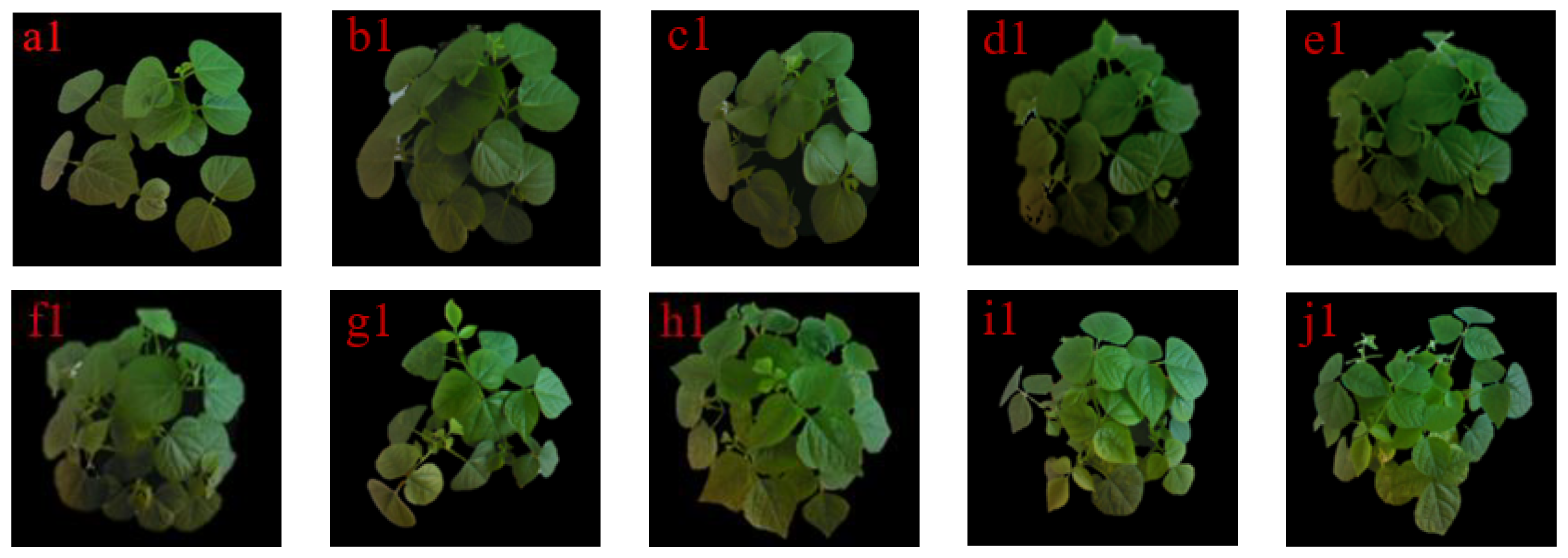
2.2.1. Extraction of the Color Canopy Images
2.2.2. Evaluation of Extraction Effect for Color Canopy Image
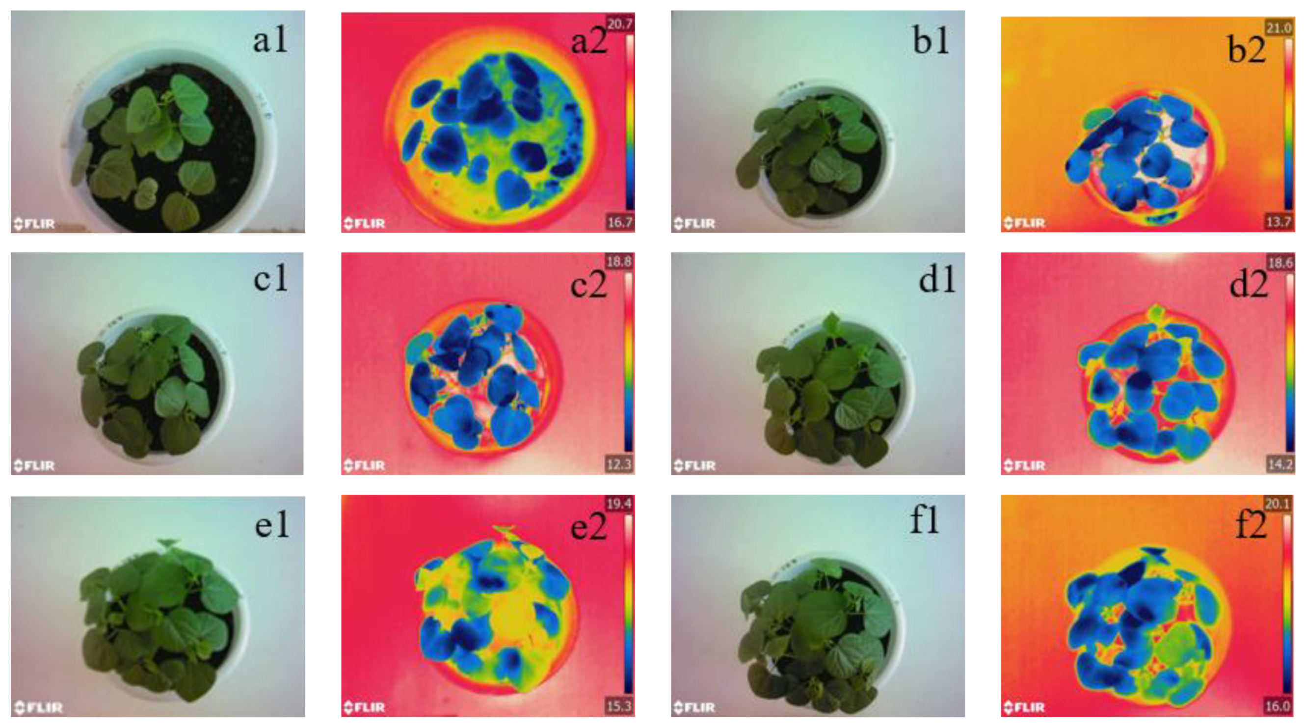
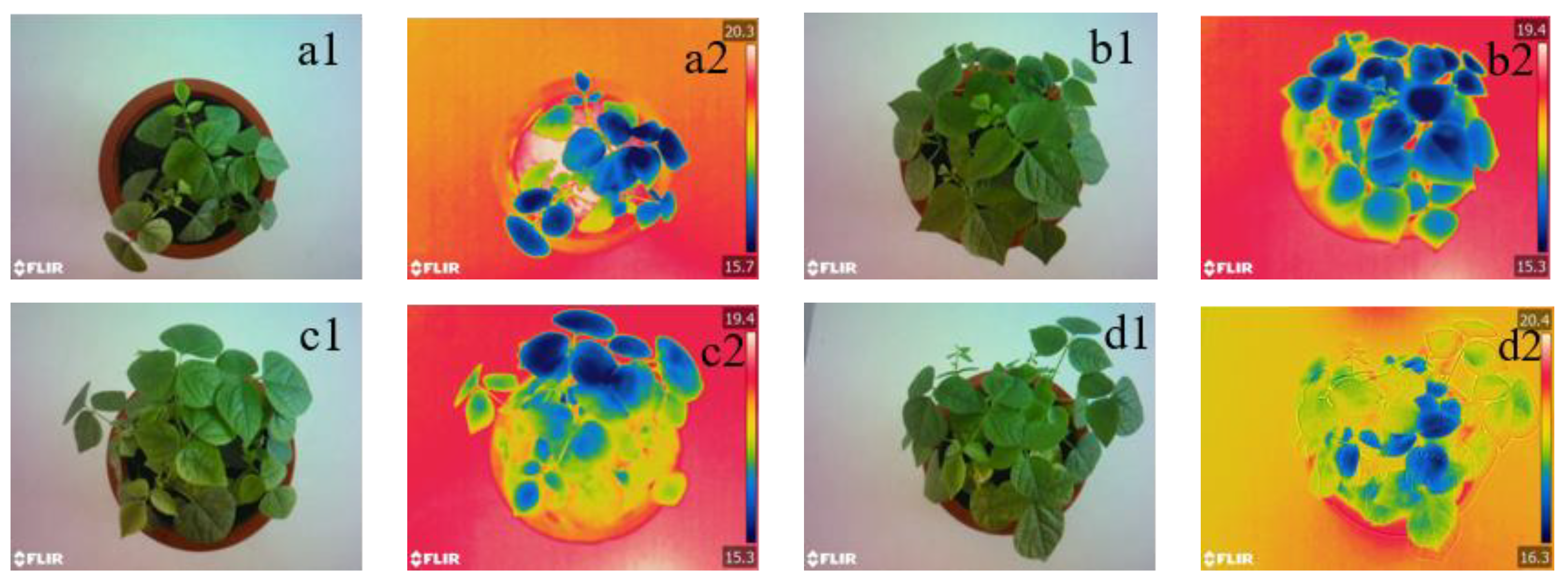
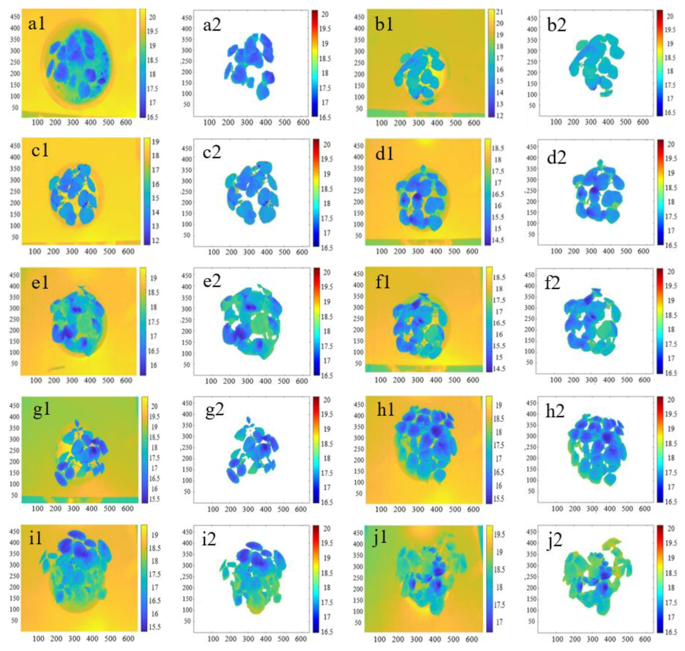
2.2.3. Extraction of the Thermal Infrared Canopy Image
2.2.4. Evaluation of Extraction Effect of the Thermal Infrared Canopy Image
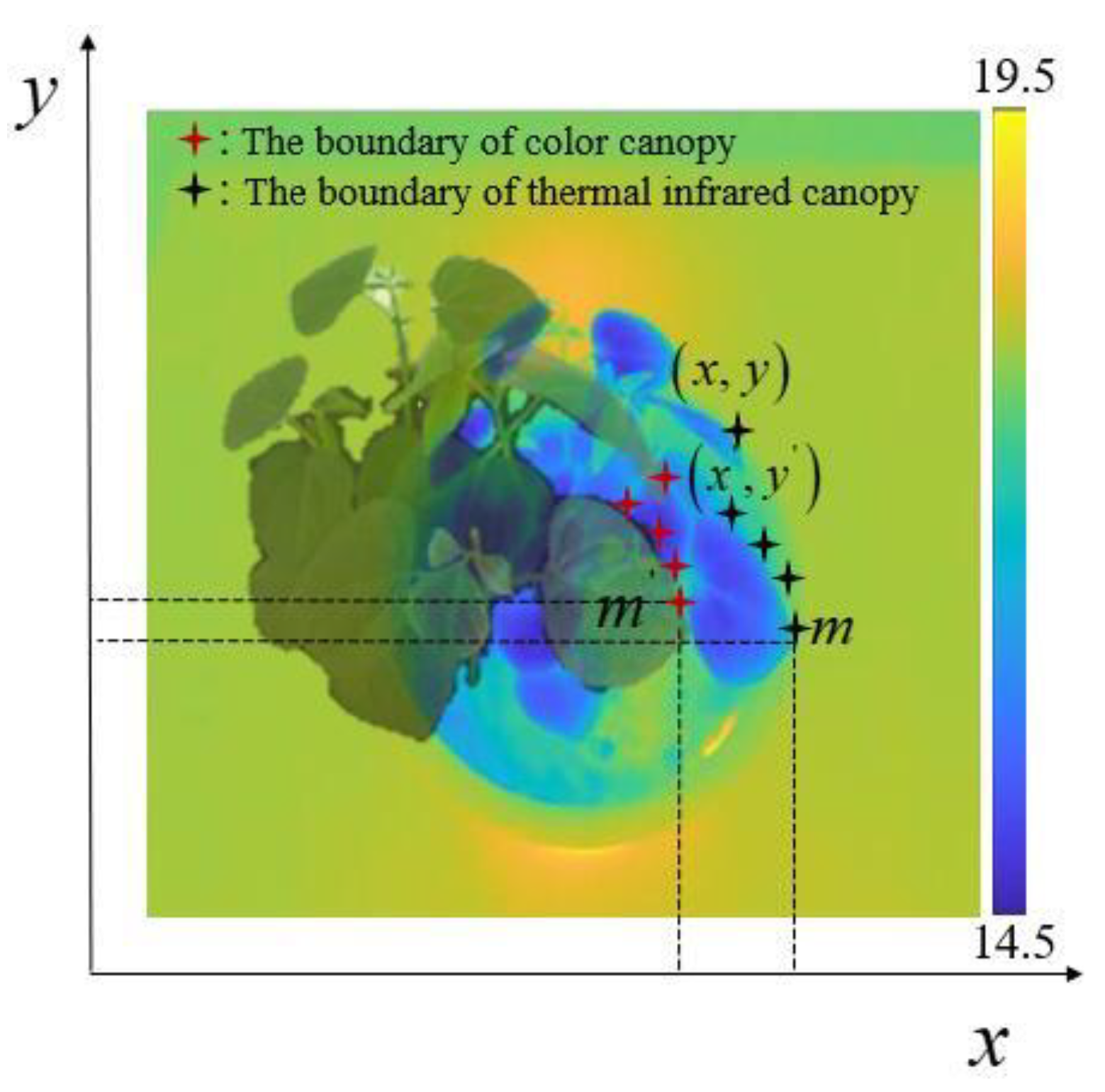
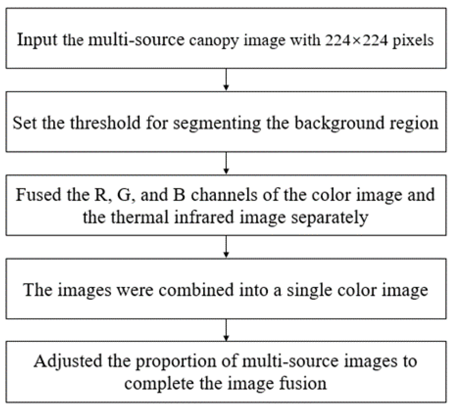
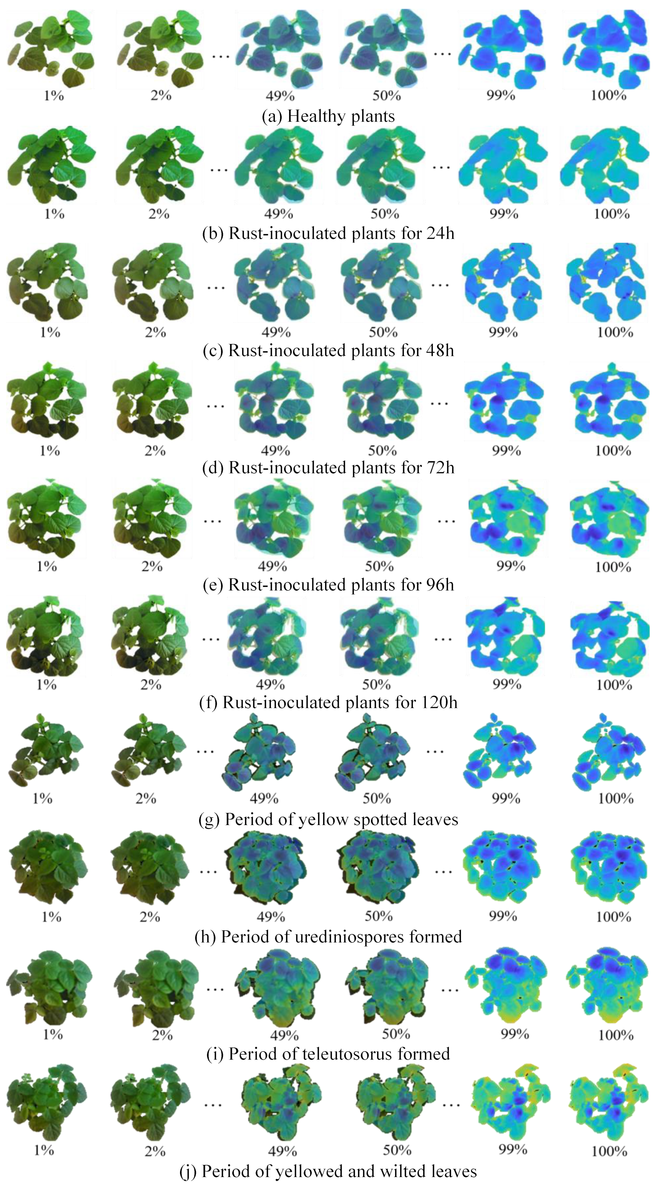
2.3. Multi-Source Image Fusion Algorithm
2.3.1. Linear Weighted Algorithm
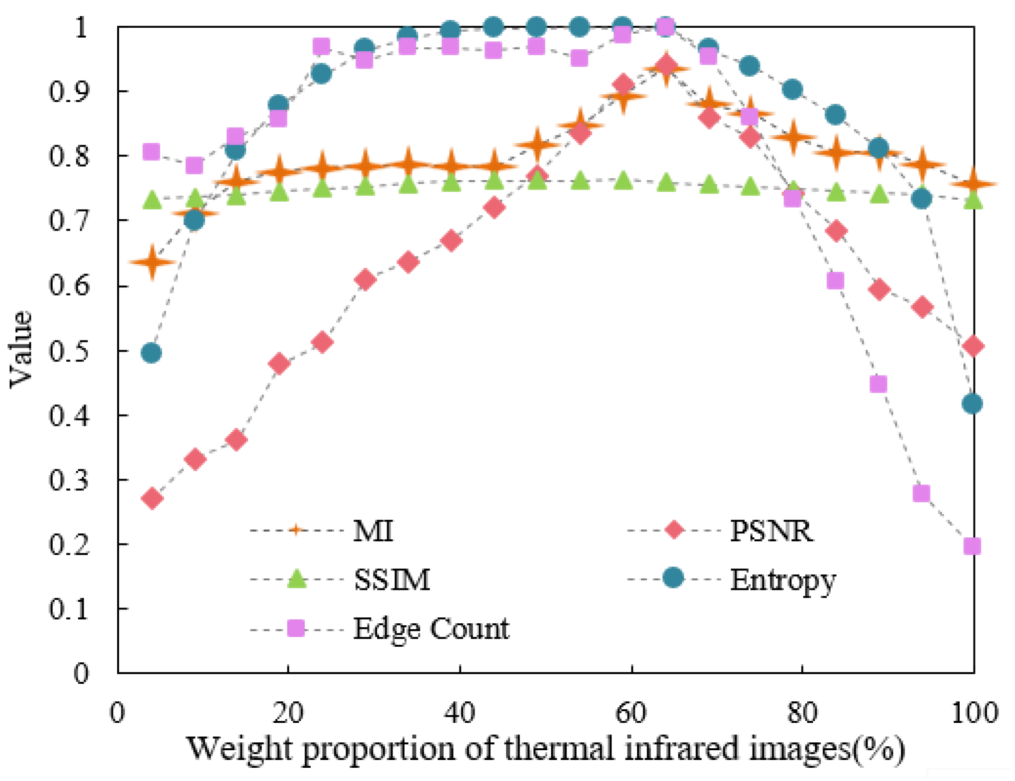
2.3.2. Evaluation of the Fusion Effect
2.4. Construction of Improved Deep Learning Model
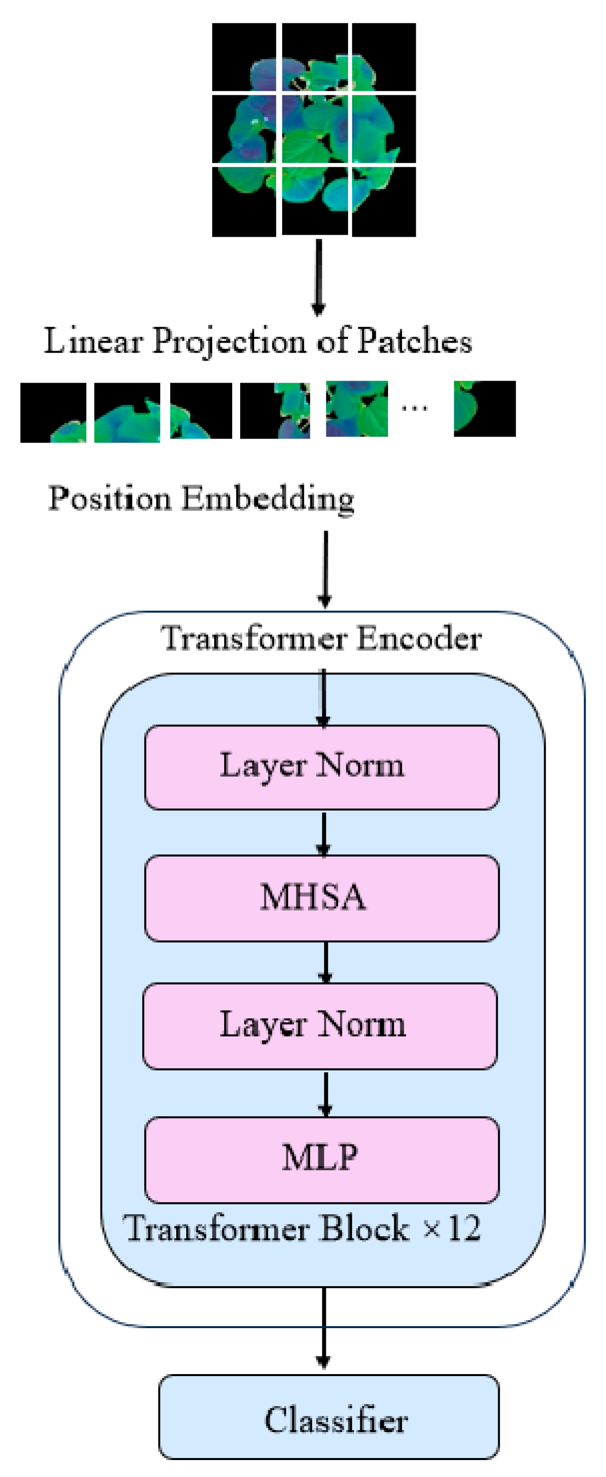
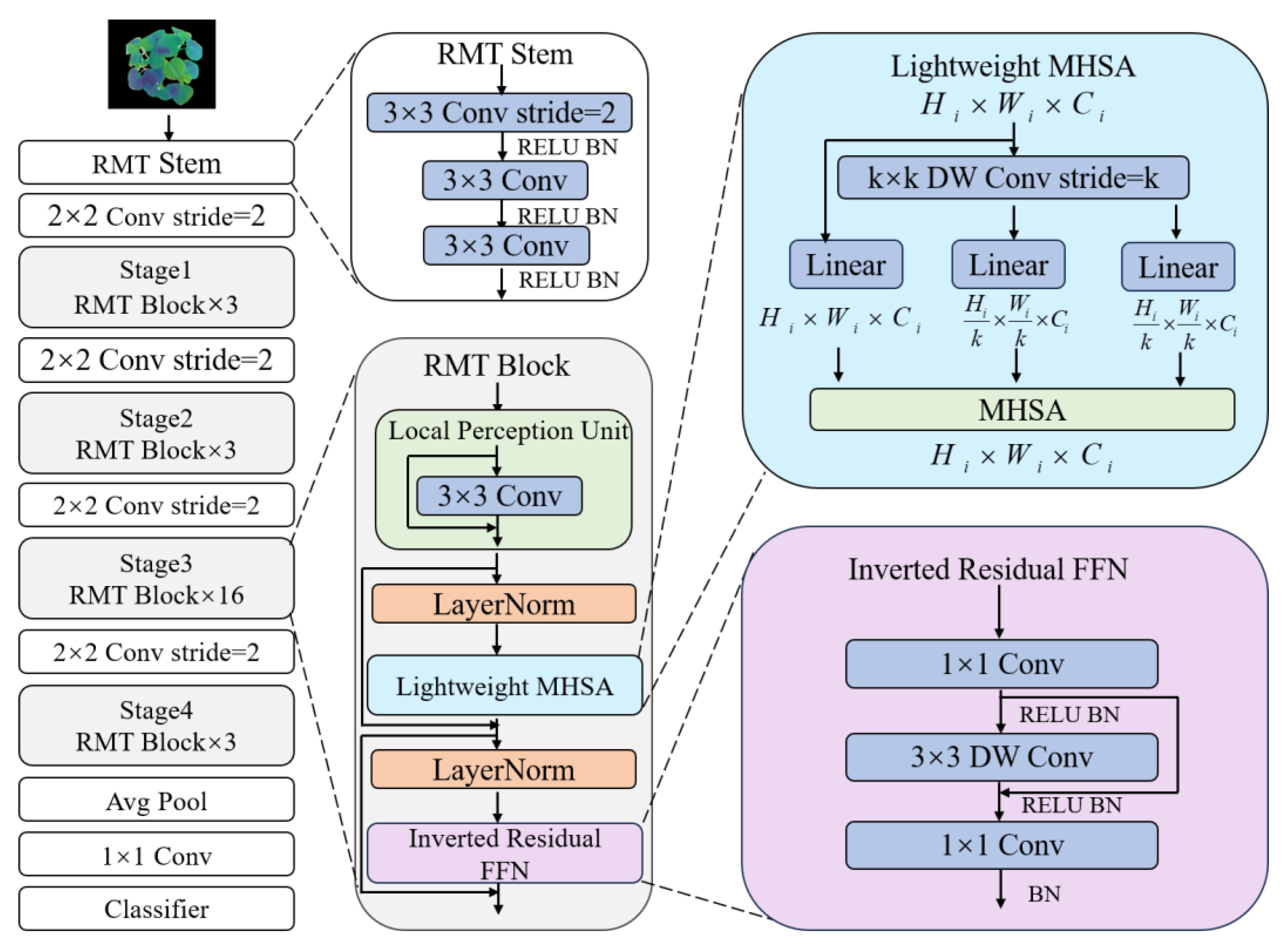
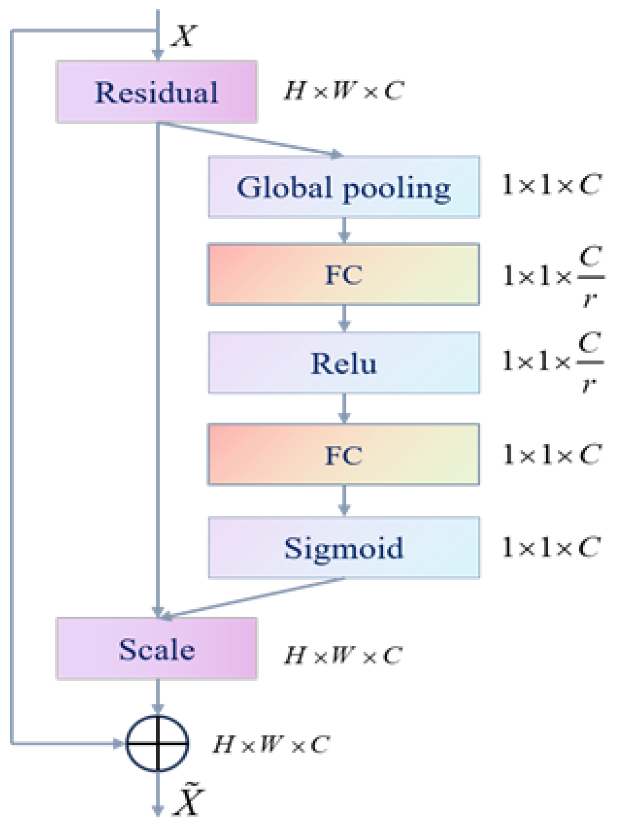
2.4.1. The ResNet-ViT Network Structure
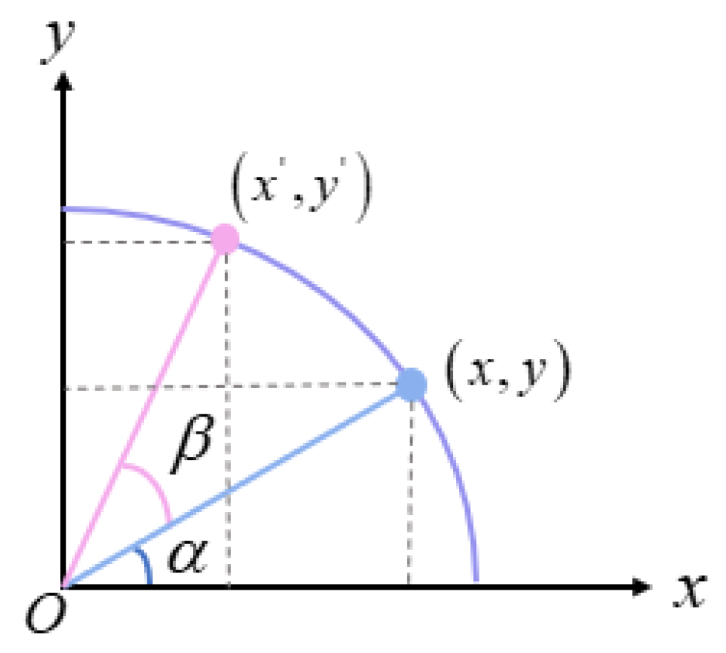
2.4.2. Optimization Algorithm
3. Results
3.1. Experimental Environment
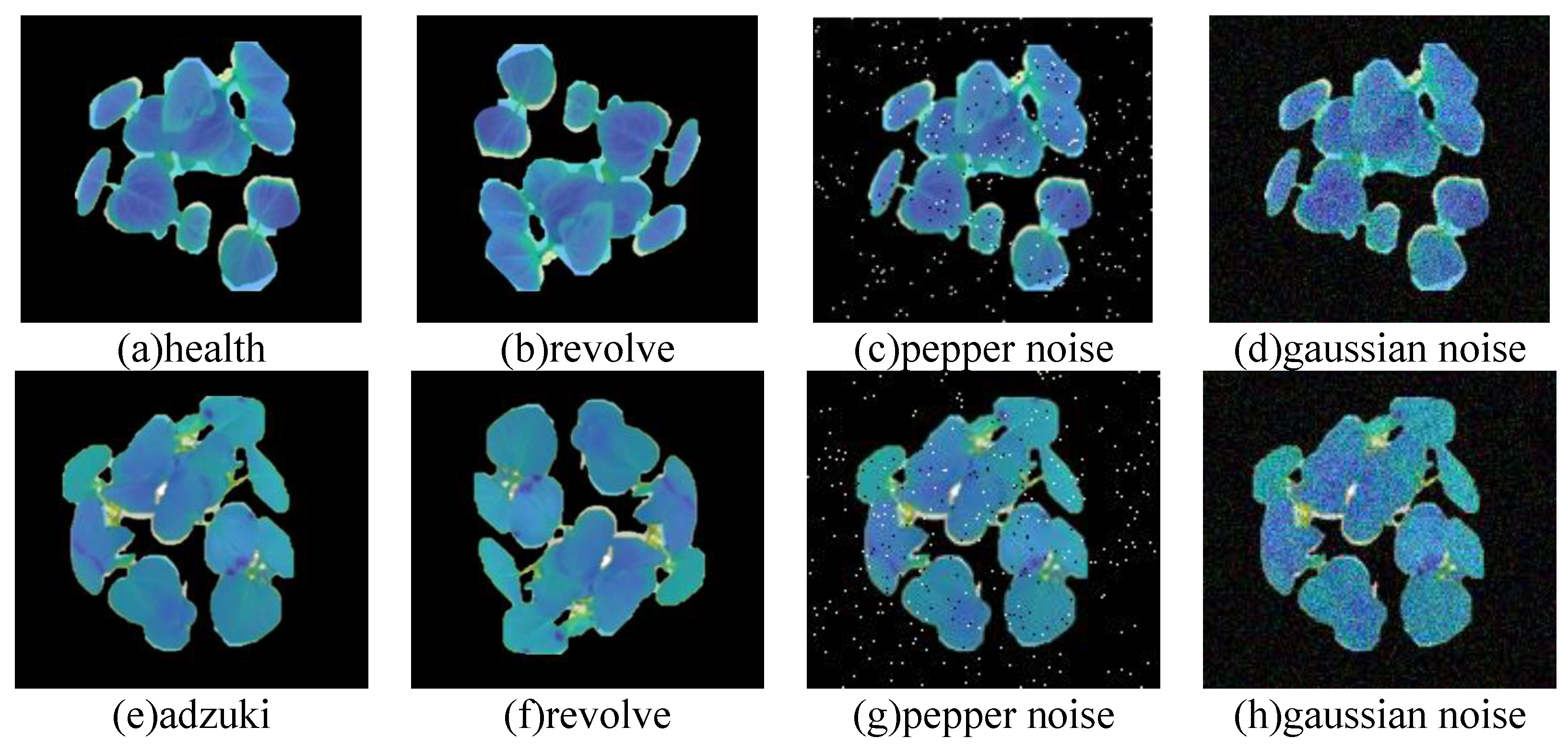
3.2. Sample Expansion and Segmentation
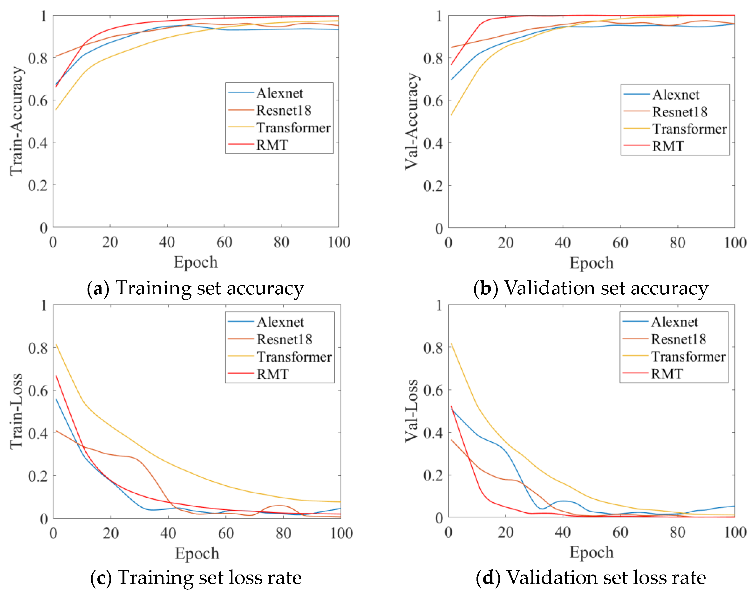
3.3. Model Training
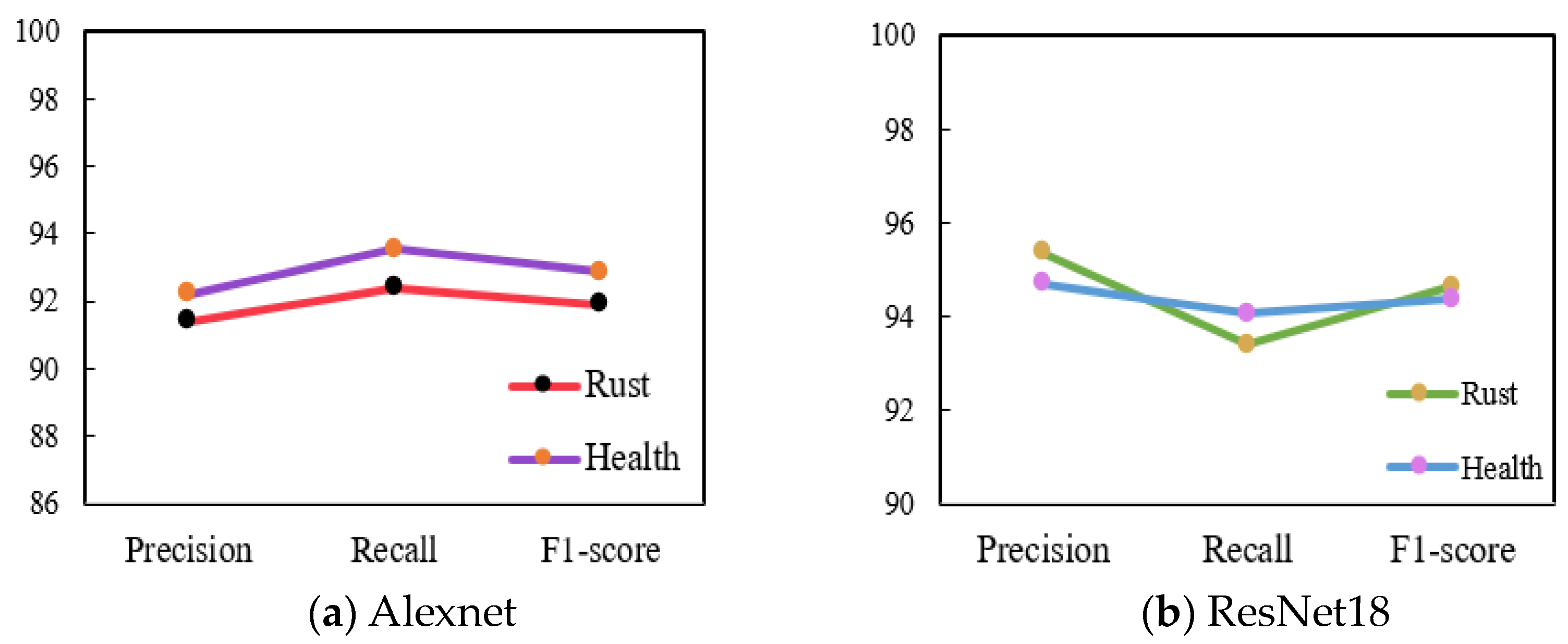
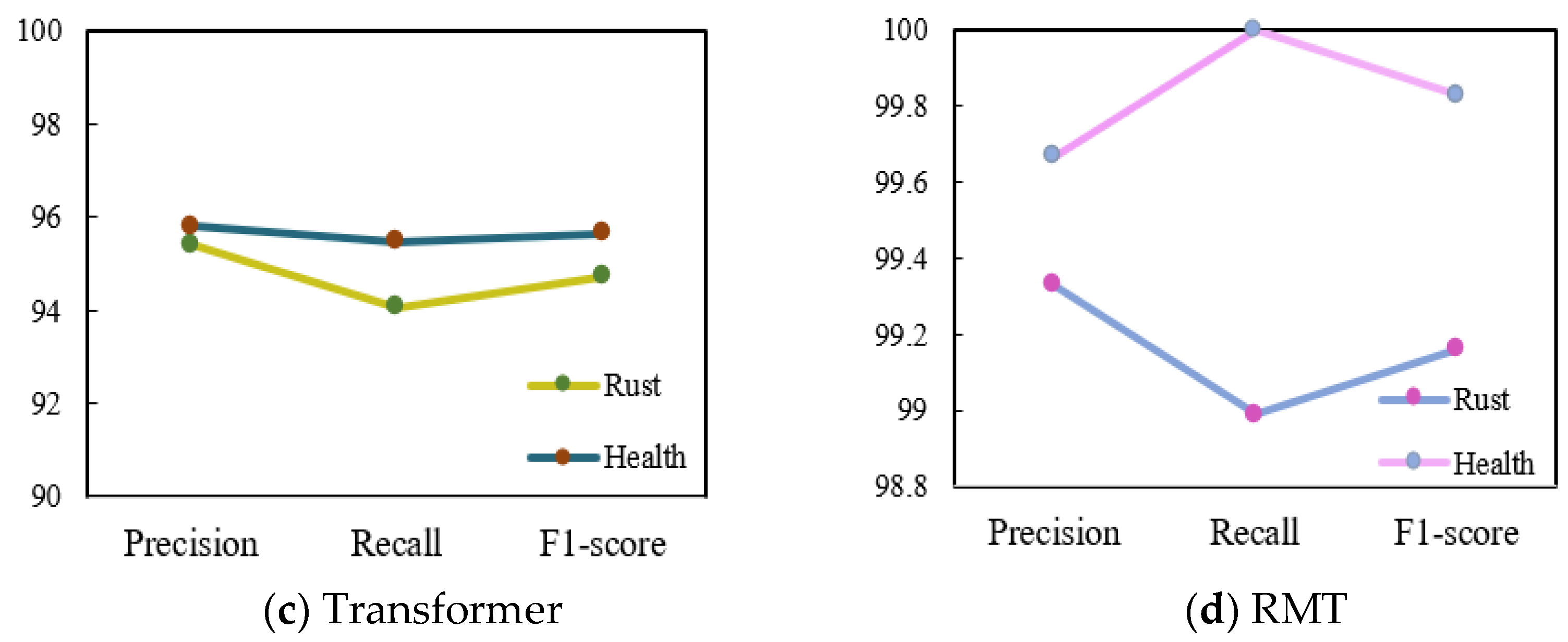
3.4. Simulation Test
4. Discussion
5. Conclusions
Author Contributions
Funding
Data Availability Statement
Conflicts of Interest
References
- Fu, X.; Ma, Q.; Yang, F.; Zhang, C.; Zhao, X.; Chang, F.; Han, L. Crop pest image recognition based on the improved ViT method. Inf. Process. Agric. 2023, 11, 249–259. [Google Scholar] [CrossRef]
- Zhang, J.; Shen, D.; Chen, D.; Ming, D.; Ren, D.; Diao, Z. ISMSFuse: Multi-modal fusing recognition algorithm for rice bacterial blight disease adaptable in edge computing scenarios. Comput. Electron. Agric. 2024, 223, 109089. [Google Scholar] [CrossRef]
- Padhi, S.; Gore, P.; Tripathi, K. Nutritional Potential of Adzuki Bean Germplasm and Mining Nutri-Dense Accessions through Multivariate Analysis. Foods 2023, 12, 4159. [Google Scholar] [CrossRef]
- Guo, B.; Ke, X.; Gao, S.; Yu, X.; Sun, Q.; Zuo, Y. A preliminary study on the mechanisms of melatonin-induced rust resistance of adzuki bean. Plant Prot. 2020, 46, 145–150. [Google Scholar] [CrossRef]
- Patil, K.; Suryawanshi, Y.; Patrawala, A. A comprehensive lemongrass (Cymbopogon citratus) leaf dataset for agricultural research and disease prevention. Data Brief 2024, 53, 110104. [Google Scholar] [CrossRef] [PubMed]
- Qu, T.; Xu, J.; Chong, Q.; Liu, Z.; Yan, W.; Wang, X.; Song, Y.; Ni, M. Fuzzy neighbourhood neural network for high-resolution remote sensing image segmentation. Eur. J. Remote Sens. 2023, 56, 2174706. [Google Scholar] [CrossRef]
- Mahadevan, K.; Punitha, A.; Suresh, J. Automatic Recognition of Rice Plant Leaf Diseases Detection using Deep Neural Network with Improved Threshold Neural Network. e-Prime-Adv. Electr. Eng. Electron. Energy 2024, 8, 100534. [Google Scholar] [CrossRef]
- Dai, G.; Tian, Z.; Fan, J. DFN-PSAN: Multi-level deep information feature fusion extraction network for interpretable plant disease classification. Comput. Electron. Agric. 2024, 216, 108481. [Google Scholar] [CrossRef]
- Kini, A.; Prema, K.; Pai, S. Early stage black pepper leaf disease prediction based on transfer learning using ConvNets. Sci. Rep. 2024, 14, 1404. [Google Scholar] [CrossRef]
- Liu, S.; Wang, Y.; Liu, H.; Sun, L.; Ma, B.; Mu, J.; Ren, Z.; Wang, J. Image Segmentation of Apple Orchard Feathering Pest Adhesion Based on Shape—Color Screening. Trans. Chin. Soc. Agric. Mach. 2024, 55, 263–274. [Google Scholar] [CrossRef]
- He, T.; Huang, Y.; Gao, H.; Zhang, Z.; Guo, R.; Yang, Y. Study on Water Stress Index Model of Lettuce Based on Fusion of Thermal Infrared and Visible Light Images. Water Sav. Irrig. 2023, 2023, 116–122. [Google Scholar] [CrossRef]
- Ma, X.; Liu, M.; Guan, H.; Wen, F.; Liu, G. Research on crop canopy identification method based on thermal infrared image processing technology. Spectrosc. Spectr. Anal. 2021, 41, 216–222. [Google Scholar] [CrossRef]
- Liu, M.; Guan, H.; Ma, X.; Yu, S.; Liu, G. Recognition method of thermal infrared images of plant canopies based on the characteristic registration of heterogeneous images. Comput. Electron. Agric. 2020, 177, 105678. [Google Scholar] [CrossRef]
- Ben, Y.; Tang, R.; Dai, P.; Li, Q. Image enhancement algorithm for underwater vision based on weighted fusion. J. Beijing Univ. Aeronaut. Astronaut. 2023, 50, 1438–1445. [Google Scholar] [CrossRef]
- Thaseentaj, S.; Ilango, S. Deep Convolutional Neural Networks for South Indian Mango Leaf Disease Detection and Classification. Comput. Mater. Contin. 2023, 77, 3593–3618. [Google Scholar] [CrossRef]
- Hernández, I.; Gutiérrez, S.; Tardaguila, J. Image analysis with deep learning for early detection of downy mildew in grapevine. Sci. Hortic. 2024, 331, 113155. [Google Scholar] [CrossRef]
- Liu, Y.; Wang, J.; Du, C.; Ding, R.; Gao, Q.; Zong, H.; Jiang, H. Detection of Various Tobacco Leaf Diseases Based on YOLOv3. Chin. Tob. Sci. 2022, 43, 94–100. [Google Scholar] [CrossRef]
- Ma, N.; Ren, Y. Identification of Various Plant Leaf Diseases Based on Multi-feature BP Neural Network. Chin. Agric. Sci. Bull. 2024, 40, 158–164. [Google Scholar] [CrossRef]
- Ashwini, C.; Sellam, V. An optimal model for identification and classification of corn leaf disease using hybrid 3D-CNN and LSTM. Biomed. Signal Process. Control 2024, 92, 106089. [Google Scholar] [CrossRef]
- Song, Z.; Lu, Y.; Ding, Z. A New Remote Sensing Desert Vegetation Detection Index. Remote Sens. 2023, 15, 5742. [Google Scholar] [CrossRef]
- Tan, J.; Xiao, W.; Ouyang, X.; Zhang, F.; Wei, X.; Jia, Z. Detection and Characterization Method of Algae on Insulator Surface Based on Vegetation Index. Environ. Technol. 2021, 39, 133–139+143. [Google Scholar] [CrossRef]
- Wen, L.; Chen, S.; Xie, M.; Liu, C.; Zhang, L. Training multi-source domain adaptation network by mutual information estimation and minimization. Neural Netw. 2024, 2024, 171353–171361. [Google Scholar] [CrossRef] [PubMed]
- Dtissibe, F.Y.; Ari, A.A.A.; Abboubakar, H.; Njoya, A.N.; Mohamadou, A.; Thiare, O. A comparative study of Machine Learning and Deep Learning methods for flood forecasting in the Far-North region, Cameroon. Sci. Afr. 2024, 23, e02053. [Google Scholar] [CrossRef]
- Tolie, H.F.; Ren, J.; Elyan, E. DICAM: Deep Inception and Channel-wise Attention Modules for underwater image enhancement. Neurocomputing 2024, 584, 127585. [Google Scholar] [CrossRef]
- Wei, X.; Li, J.; Chen, G. Image Quality Estimation Based on Multi-linear Analysis. J. Image Graph. 2008, 13, 2123–2131. [Google Scholar] [CrossRef]
- Wang, Y.; Wu, M.; Geng, F.; Feng, Y.; Zhou, W. Underwater image enhancement algorithm based on image entropy linear weighting. J. Chongqing Technol. Bus. Univ. 2023, 1–8. Available online: http://kns.cnki.net/kcms/detail/50.1155.N.20230524.1059.002.html (accessed on 10 July 2024).
- Xie, X.; Cheng, W. Method of infrared thermal imaging and visible light image fusion based on U2⁃Net. Mod. Electron. Tech. 2024, 47, 100–104. [Google Scholar] [CrossRef]
- Gao, S.; Jin, W.; Wang, L.; Luo, Y.; Li, J. Quality evaluation for dual-band color fusion images based on scene understanding. Infrared Laser Eng. 2014, 43, 300–305. [Google Scholar] [CrossRef]
- Tang, Z.; Li, J.; Huang, J.; Wang, Z.; Luo, Z. Multi-scale convolution underwater image restoration network. Mach. Vis. Appl. 2022, 33, 85. [Google Scholar] [CrossRef]
- Lin, Y.; Zhou, J.; Ren, W.; Zhang, W. Autonomous underwater robot for underwater image enhancement via multi-scale deformable convolution network with attention mechanism. Comput. Electron. Agric. 2021, 191, 106497. [Google Scholar] [CrossRef]
- Ma, H.; Zhang, Y.; Sun, S.; Zhang, W.; Fei, M.; Zhou, H. Weighted multi-error information entropy based you only look once network for underwater object detection. Eng. Appl. Artif. Intell. 2024, 130, 107766. [Google Scholar] [CrossRef]
- Luo, X.; Wang, J.; Zhang, Z.; Wu, X.J. A full-scale hierarchical encoder-decoder network with cascading edge-prior for infrared and visible image fusion. Pattern Recognit. 2024, 148, 110192. [Google Scholar] [CrossRef]
- Fang, J.; Liu, H.; Mu, X. Self-supervised monocular depth estimation based on convolution neural network hybrid transformer. Intell. Comput. Appl. 2024, 14, 168–174+179. [Google Scholar] [CrossRef]
- Dwivedi, K.; Dutta, M.K.; Pandey, J.P. EMViT-Net: A novel transformer-based network utilizing CNN and multilayer perceptron for the classification of environmental microorganisms using microscopic images. Ecol. Inform. 2024, 79, 102451. [Google Scholar] [CrossRef]
- Thwal, C.M.; Nguyen, M.N.; Tun, Y.L.; Kim, S.T.; Thai, M.T.; Hong, C.S. OnDev-LCT: On-Device Lightweight Convolutional Transformers towards federated learning. Neural Netw. 2024, 170, 635–649. [Google Scholar] [CrossRef] [PubMed]
- Tian, Y.; Zhang, Y.; Zhang, H. Recent advances in stochastic gradient descent in deep learning. Mathematics 2023, 11, 682. [Google Scholar] [CrossRef]
- Setiawan, A.; Yudistira, N.; Wihandika, R.C. Large scale pest classification using efficient Convolutional Neural Network with augmentation and regularizers. Comput. Electron. Agric. 2022, 200, 107204. [Google Scholar] [CrossRef]
- Yu, M.; Ma, X.; Guan, H. Recognition method of soybean leaf diseases using residual neural network based on transfer learning. Ecol. Inform. 2023, 76, 102096. [Google Scholar] [CrossRef]
- Makomere, R.S.; Koech, L.; Rutto, H.L.; Kiambi, S. Precision forecasting of spray-dry desulfurization using Gaussian noise data augmentation and k-fold cross-validation optimized neural computing. J. Environ. Sci. Health Part A 2024, 59, 1–14. [Google Scholar] [CrossRef]
- Krizhevsky, A.; Sutskever, I.; Hinton, G.E. ImageNet classification with deep convolutional neural networks. Commun. ACM 2017, 60, 84–90. [Google Scholar] [CrossRef]
- He, K.; Zhang, X.; Ren, S.; Sun, J. Identity Mappings in Deep Residual Networks. In Proceedings of the Computer Vision—ECCV 2016—14th European Conference, Amsterdam, The Netherlands, 11–14 October 2016; pp. 630–645. [Google Scholar] [CrossRef]
- Han, K.; Wang, Y.; Chen, H.; Chen, X.; Guo, J.; Liu, Z.; Tang, Y.; Xiao, A.; Xu, C.; Xu, Y.; et al. A Survey on Vision Transformer. IEEE Trans. Pattern Anal. Mach. Intell. 2020, 45, 87–110. [Google Scholar] [CrossRef]
- Yu, M.; Ma, X.; Guan, H.; Liu, M.; Zhang, T. A recognition method of soybean leaf diseases based on an improved deep learning model. Front. Plant Sci. 2022, 13, 878834. [Google Scholar] [CrossRef] [PubMed]
- Yu, M.; Ma, X.; Guan, H.; Zhang, T. A diagnosis model of soybean leaf diseases based on improved residual neural network. Chemom. Intell. Lab. Syst. 2023, 237, 104824. [Google Scholar] [CrossRef]
- Xie, Q.; Sun, W.; Shen, Z. Segmentation of photovoltaic infrared hot spot image based on gray level clustering. Acta Energiae Solaris Sin. 2023, 44, 117–124. [Google Scholar] [CrossRef]
- Hao, S.; Li, J.; Ma, X.; He, T.; Sun, S.; Li, T. Infrared and Visible Image Fusion Algorithm Based on Feature Optimization and GAN. Acta Photonica Sin. 2023, 52, 1210004. [Google Scholar] [CrossRef]
- Li, J.; Liu, Z.; Wang, D. A Lightweight Algorithm for Recognizing Pear Leaf Diseases in Natural Scenes Based on an Improved YOLOv5 Deep Learning Model. Agriculture 2024, 14, 273. [Google Scholar] [CrossRef]
- Si, H.; Li, M.; Li, W.; Zhang, G.; Wang, M.; Li, F.; Li, Y. A Dual-Branch Model Integrating CNN and Swin Transformer for Efficient Apple Leaf Disease Classification. Agriculture 2024, 14, 142. [Google Scholar] [CrossRef]
- Wang, F.; Rao, Y.; Luo, Q.; Jin, X.; Jiang, Z.; Zhang, W.; Li, S. Practical cucumber leaf disease recognition using improved Swin Transformer and small sample size. Comput. Electron. Agric. 2022, 199, 107163. [Google Scholar] [CrossRef]
- Ding, R.; Qiao, Y.; Yang, X.; Jiang, H.; Zhang, Y.; Huang, Z.; Liu, H. Improved ResNet based apple leaf diseases identification. IFAC-Pap. 2022, 55, 78–82. [Google Scholar] [CrossRef]
- Kumar, S.; Pal, S.; Singh, V.P.; Jaiswal, P. Performance evaluation of ResNet model for classification of tomato plant disease. Epidemiol. Methods 2023, 12, 20210044. [Google Scholar] [CrossRef]
- Xie, F.; Qi, T.; Zhang, P. Design of infrared detection sensitivity test equipment based on double black body. In Eighth Symposium on Novel Photoelectronic Detection Technology and Applications; SPIE: Bellingham, WA, USA, 2022; pp. 2301–2305. [Google Scholar] [CrossRef]


| Extraction Method | DEXG Algorithm | |
|---|---|---|
| Evaluation Indicators | ||
| DICE | 0.9971 | |
| OE | 0.0016 | |
| Jaccard | 0.9869 | |
| Canopy Extraction Methods | Canopy Extraction Evaluation Indicators | ||
|---|---|---|---|
| OR | UR | SA | |
| Affine transformation | 0.0026 | 0.0193 | 0.9785 |
| Status of Adzuki Beans | Number of Training Sets | Number of Validation Sets | Number of Test Sets |
|---|---|---|---|
| Rust disease | 9207 | 2630 | 1315 |
| Healthy | 8853 | 2529 | 1264 |
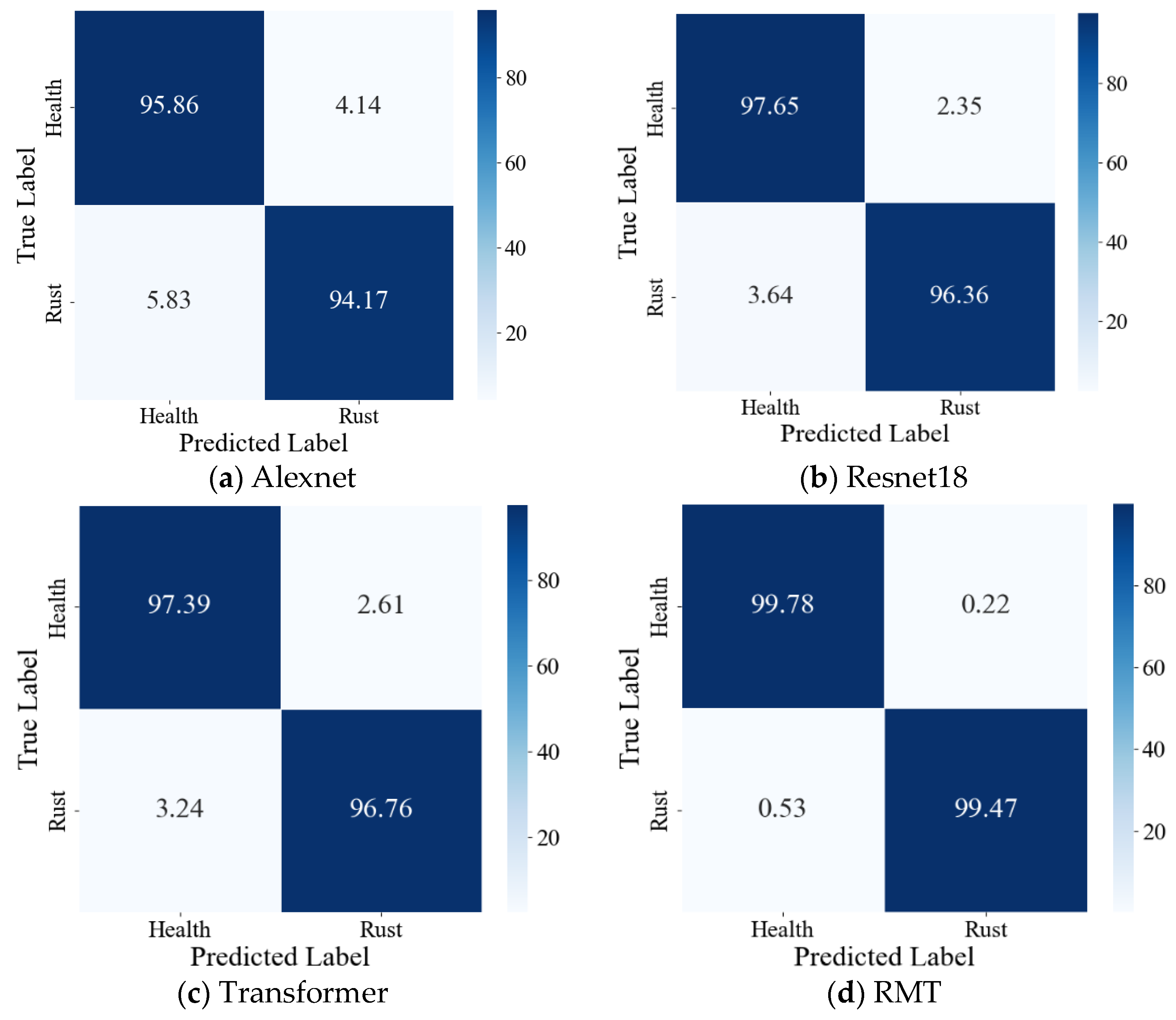
| Plant Condition | Accuracy/% | |||
|---|---|---|---|---|
| Alexnet | ResNet18 | Transformer | RMT | |
| Rust disease | 94.17% | 96.36% | 96.76% | 99.47% |
| Healthy | 95.86% | 97.65% | 97.39% | 99.78% |
| Average value | 95.01% | 97.00% | 97.08% | 99.63% |
| Algorithmic Model | Alexnet | ResNet18 | Transformer | RMT | |
|---|---|---|---|---|---|
| Performance Index | |||||
| Model size/MB | 55.69 | 72.76 | 127.35 | 61.26 | |
| Average recognition time/s | 0.086380 | 0.073682 | 0.138329 | 0.072184 | |
Disclaimer/Publisher’s Note: The statements, opinions and data contained in all publications are solely those of the individual author(s) and contributor(s) and not of MDPI and/or the editor(s). MDPI and/or the editor(s) disclaim responsibility for any injury to people or property resulting from any ideas, methods, instructions or products referred to in the content. |
© 2024 by the authors. Licensee MDPI, Basel, Switzerland. This article is an open access article distributed under the terms and conditions of the Creative Commons Attribution (CC BY) license (https://creativecommons.org/licenses/by/4.0/).
Share and Cite
Ma, X.; Zhang, X.; Guan, H.; Wang, L. Recognition Method of Crop Disease Based on Image Fusion and Deep Learning Model. Agronomy 2024, 14, 1518. https://doi.org/10.3390/agronomy14071518
Ma X, Zhang X, Guan H, Wang L. Recognition Method of Crop Disease Based on Image Fusion and Deep Learning Model. Agronomy. 2024; 14(7):1518. https://doi.org/10.3390/agronomy14071518
Chicago/Turabian StyleMa, Xiaodan, Xi Zhang, Haiou Guan, and Lu Wang. 2024. "Recognition Method of Crop Disease Based on Image Fusion and Deep Learning Model" Agronomy 14, no. 7: 1518. https://doi.org/10.3390/agronomy14071518
APA StyleMa, X., Zhang, X., Guan, H., & Wang, L. (2024). Recognition Method of Crop Disease Based on Image Fusion and Deep Learning Model. Agronomy, 14(7), 1518. https://doi.org/10.3390/agronomy14071518