The Effects of Global Warming on Agroclimatic Regions in China: Past and Future

Abstract

Agroclimatic regionalization is an effective way to utilize agricultural climate resources in a reasonable manner. Accurate and objective agroclimatic regionalization plays a great directive role in ecological layout and decision support for agriculture farming. The purpose of this article was to investigate the influence of climate change on agroclimatic regions in China. Following the same regionalization principle concept as the theory and techniques of agroclimatic regionalization, three agroclimatic regions, the Tibetan High Cold Region (THCR), Northwest Arid Region (NAR), and Eastern Monsoon Region (EMR) were identified in China. The changes in the three agroclimatic regions were analyzed from 1961 to 2020 in the past and from 2006 to 2060 in the future. Future changes in agroclimatic regions were estimated from 2006 to 2030 and from 2031 to 2060 under scenarios RCP2.6, RCP4.5, and RCP8.5 for greenhouse gas emissions. The borders of agoclimatic regions had changed as a result of global climate warming and precipitation variability. There was a surplus in the geographical displacement and range of agroclimatic region borders in 1991 to 2020, especially when compared to those in 1961–1990. The TCHR exhibited significant spatial variation, with its northeast corner shifting nearly 170 km to the southwest. In the future, the area ratio of the THCR will be 26% by 2031–2060 under the RCP8.5 scenario, with the highest decline (1% compared to that in the reference period of 1981–2005), while under the RCP4.5 and RCP2.6 scenarios it will stabilize the area ratio at 27%. The eastern boundary of the NAR will migrate south or east, while the center boundary will rise northward. Under all three climatic scenarios, the area ratio will be 25% (down 1%). The range of the EMR will expand. The area ratio of the EMR will increase by 1% under the RCP2.6 and RCP4.5 scenarios and by 2% under the RCP8.5 scenario. Overall, our study may facilitate an in-depth understanding of agroclimatic regions changes and thus provide a scientific reference for the distribution of agricultural production and sustainable development under climate change in China.

1. Introduction

Agroclimatic regionalization is a specialized method of dividing regions that reflects the relationship between agricultural production and climate. It serves as a valuable tool for the rational allocation of agricultural resources, enhancement of farming systems, and introduction and promotion of improved varieties [1]. According to the Fourth Report of the Intergovernmental Pannel on Climate Change (IPCC), the global surface temperature has increased by 0.74 °C in the past 100 years, with particularly notable increases observed in the high latitude of the northern hemisphere [2]. The changes in climate resources and their impact on agriculture have received considerable attention. Over the years, many scholars at home and abroad have conducted extensive research on agroclimatic regionalization, aiming to grasp the spatiotemporal distribution patterns and trends of climate resources, and provide a scientific basis for the rational use of climate resources [3,4,5,6].

In actual research, appropriate zoning indicators can be directly selected based on long-term agricultural practice and experience, or agricultural climate resource analysis can be utilized to determine the climatic conditions for crop growth and development by employing climate data, crop yield, area, disaster records, and other relevant data. These approaches involve statistical analysis and biological methods, as well as field experiments. Some qualitative key agroclimatic parameters, such as an accumulated temperature of above 0 °C or 10 °C and the length of temperature growing periods, the humidity index, and the length of the growing period, were selected to analyze agroclimatic zoning [4,7,8]. The agroclimatic regionalization indices can also be established and enhanced through the comparison of agrometeorological survey data with corresponding meteorological data collected during the same period, or by comparing crop data gathered from field experiments with corresponding meteorological data [9,10,11,12]. For instance, based on years of agricultural meteorological data, an empirical equation was derived to calculate the temperature risk of frost (F) for wheat after the jointing stage, and F was used as an indicator to achieve agroclimatic zoning for wheat frost in the Huanghuai wheat region [13]. Specific models such as the Agro-Ecological Zone model was applied to develop the agro-ecological zoning of chickpea in semi-arid regions of Iran based on GIS [10]. Previous studies have demonstrated a substantial increase in annual mean surface temperatures over the past 100 years [2]. As a consequence of climate change, there have been notable alterations in agricultural climatic resources. Poland [14], Canada [15,16], and other continents [17,18] have observed significant changes in agroclimatic indices related to crop growth, such as the duration and the timing of the growing season. Furthermore, future climate scenario predictions included continued warming throughout China’s climate during the 21st century, particularly the northern winter half-year, accompanied by an increasing tendency of precipitation [19]. Chu et al. [3] predicted that Northeast China would experience an earlier onset of accumulated temperatures reaching 10 °C, longer frost seasons, and extended agricultural growing seasons. These anticipated climate changes would also impact crop distribution patterns and agricultural planting boundaries. Yang et al. [20]’s predictions indicated that the national planting system would shift northward to varied extents between 2011–2040 and 2041–2050. While tropical crops’ northern limits for cultivation would move northwards accordingly, those for winter wheat would shift northward while expanding westward. Currently, limited reports exist that quantitatively compare the impacts of future climate change on agroclimatic regions in China. Therefore, it is imperative to employ reliable climate scenario data for estimating future agroclimatic regions to obtain more insights into agroclimatic region transformations.

Analysis of changes in agroclimatic regions provides important information for scientists, agricultural policy makers, producers, and others. The analysis result helps them make appropriate decisions about policies and management practices, and also helps them adapt those policies to minimize the adverse effect of climate change. In the past, agroclimatic regionalization studies and results were often carried out in limited regions or at a few climatic observation sites. The original agroclimatic regionalization cannot adequately reflect the geographical and temporal system changes of agroclimatic regions and adapt to the actual needs of modern agricultural production. Understanding changes in agroclimatic regions in the past and identifying their future development trends are useful in determining the regional susceptibility to special conditions.

This study focused on historical and future changes in agroclimatic regions. In order to investigate the alterations in agroclimatic regions, the indices of agroclimatic regionalization were computed from 1961 to 2020. By comparing observed data and simulated data discrepancies, climate projections for the next 60 years were derived based on three greenhouse gas emission scenarios: RCP2.6, RCP4.5, and RCP8.5. Subsequently, employing the same index methodology, agroclimatic regions in China during the early and middle 21st century were delineated. The main aim of this study was to (1) investigate the characteristics and influencing factors behind changes in China’s agroclimatic regions from 1961 to 2020; (2) provide a scientific basis for adjusting China’s planting layout and ensuring national food security by estimating regional changes in China’s agroclimatic regions under future emission scenarios.

2. Materials and Methods

2.1. Data

Meteorological data used in this study were based on daily (1961–2020) precipitation, average wind speed, and maximum, minimum, and average temperature (from National Climatic Center, China). Some observation stations with a large amount of data missing and poor coherence in data time series were eliminated. Finally, data of 1487 meteorological stations, except stations in Taiwan province, were selected for agroclimatic regionalization. The period was subdivided into 1961–1990 (period I), 1971–2000 (period II), 1981–2010 (period III) and 1991–2020 (period IV). Basic geographic information data included the administrative boundary and elevation.

The main climatic factors to be used in this study were active accumulated temperature above 0 °C (hereinafter referred to as accT0) [21], the average temperature of the hottest July (Th), the annual mean precipitation (R), and the number of days with a daily wind speed greater than 5 m/s (D_w). R, Th, and D_w were calculated using daily meteorological data. To display the spatial variation in agroclimatic indices, ArcGIS 10.6 software was employed to perform spatial interpolation (inverse-distance weighted interpolation) for R and D_w. accT0 and Th were interpolated using the ANUSPLIN method (version 4.2) [22], which took into account the effects of altitude on the temperature. The spatial resolution of interpolation was 5 km in a Asia North Albers Equal Area Conic projection. The indices and standards for the agroclimatic regions are shown in

Table 1. Indices for the agroclimatic regions.

Agroclimatic Region	Dominant Indices	Supplementary Indices	Reference Indices
Northwest Arid Region (NAR)	Accumulated frequency of 50% for 400 mm annual precipitation	Annual average days of average daily wind speed for above 5 m/s	Wind erosion and soil erosion at the boundary
Tibetan High Cold Region (THCR)	accT0 of 3000 °C·d, Th of 18 °C		Contour line (3000 m elevation) in the eastern part of the plateau
Eastern Monsoon Region (EMR)	The western part of this region was adjacent to the NAR and the THCR from north to south.

.

2.2. Simulation Data

The climate change simulation data used in this paper were simulated using the regional climate model RegCM4. The horizontal resolution of the mode was 25 km, and specific parameter settings can be found in Han and Tong [23,24]. The initial and lateral boundary conditions required for RegCM4 simulation were obtained from three general circulation models, namely HadGEM2–ES, MPI–ESM–MR and NorESM1–M. The simulation data used in this article included three greenhouse gas (GHG) emission scenarios for RCP2.6, RCP4.5 and RCP8.5, with 1981 to 2005 as the contemporary period (reference period, Iens), 2006 to 2030 as the early 21st century (IIens), and 2031 to 2060 as the mid-21st century (IIIens). Referring to the analytical method of the IPCC Fifth Assessment Report [25], the RegCM4 simulation results driven by three global models were collectively averaged using an arithmetic mean with equal weights. Simulation data were represented by ensT0 (ensembled accT0), ensTh (ensembled Th), ensR (ensembled R), and ensD_w (ensembled D_w).

2.3. Methodology

The overall activity temperature of a crop during a specific time or growth season is known as active accumulated temperature. It is the primary index of heat resources of a region and the heat required for the growth and development of crops. The active cumulated temperature (accT0) refers to the total temperature, which can be calculated by summing up the daily average temperatures across a range of 0 °C or higher [21].

$$accT0=\begin{array}{cc}{\displaystyle \sum _{i=1}^{n}T}& T>0\end{array}$$

(1)

In Equation (1), accT0 is the active accumulated temperature, and °C·d, T is daily average temperature in °C.

Precipitation frequency is defined as the proportion of the number of times a specific boundary precipitation happens within a given time period compared to the overall number of precipitation occurrences within the same time period. The accumulated frequency of precipitation is the sum of the frequencies above (or below) a particular boundary precipitation. The probability of occurrence of specific-boundary precipitation is represented by the accumulated frequency of precipitation. As a border indication between the NAR and the EMR in China, this study used a 50% accumulated frequency of annual precipitation of 400 mm [1,7].

$$\alpha =\frac{\overline{R}-400}{\sigma }$$

(2)

In Equation (2), $\overline{R}$ is the annual mean precipitation for each period (I to IV) in mm; $\sigma$ is the standard deviation; $\alpha$ is the standardization coefficient. According to the relationship between the standardization coefficient and accumulated frequency of precipitation [26], the standardization coefficient corresponding to an accumulated frequency of 50% for 400 mm of annual precipitation can be determined as 0, that is, the contour line with a calculated value of 0 is the NAR boundary. The annual mean precipitation over many years follows a normal distribution, which has been verified in some regions of China [7,26]. A normality test (Kolmogorov–Smirnov) on the annual precipitation showed that 77% of the 1487 meterological stations had a normal distribution, accounting for the vast majority of the stations used. To maintain consistency, Equation (2) was used for uniform calculation.

In order to assess the accuracy of simulation data using the three general circulation models, the period from 1981 to 2005 was selected as the reference period to evaluate the simulation data and observation data. The observation data were interpolated to a 25 km grid to analyze the correlation between these two data. The correlation coefficient is a commonly used evaluation indicator, and the spatial correlation coefficient (SCOR) can be used to evaluate the simulation effect of spatial distribution. The closer the S value is to 1, the better the simulation effect. The Taylor score is a quantitative indicator of the Taylor plot and is widely used for pattern performance evaluation [23,27]. It integrates three evaluation indices, namely the spatial correlation coefficient, root mean square deviation, and standard deviation, and the calculation formula is as follows:

$$T=\frac{{\left(1+r\right)}^2}{\left(\hat{\sigma }+\frac{1}{\hat{\sigma }}\right)}$$

(3)

In the Formula (3), T is the Taylor score value, r is the spatial correlation coefficient between the simulated value and the observed value, and $\hat{\sigma }$ is the standardized spatial standard deviation (the ratio of the simulated value of standard deviation to the observed value of standard deviation). The higher the T value, the better the simulation performance. Due to the spatial resolution of the simulated data being 25 km, in order to maintain consistency with the spatial resolution of simulated data, the observed data from 1981 to 2005 were spatially interpolated and resampled to 25 km. Then, the correlation, including statistical characteristic values (maximum, minimum, and standard deviation) of each layer and their correlation coefficient were calculated between simulated and observed data grid layers using the spatial analyst tools in ArcGIS.

The coefficient of variation (CV) was introduced to reflect the relative fluctuation of precipitation changes in China under the future climatic scenarios. The larger the value, the more unstable the precipitation; the smaller the value, the more stable the precipitation. The ratio of the mean square deviation (standard deviation) to the mean, which can be expressed as a percentage, is the coefficient of variation, and is often referred to as the coefficient of deviation. The following formula can be used to calculate this:

$$\mathrm{CV}=\frac{\sigma }{\overline{R}}\times 100\%$$

(4)

In Equation (4), CV stands for the coefficient of variation. $\overline{R}$ is the mean precipitation for each period (IIens and IIIens) in mm; $\sigma$ is the standard deviation.

2.4. The Principle of Agroclimatic Regionalization

The concepts of agroclimatic regionalization were used to build a regionalization methodology, choose regionalization indices, and establish a regionalization system [28,29,30]. The following ideas led the regionalization of the agroclimate. Agroclimatic regional indices had clear and important significance. The indices revealed regional differences in agriculture productivity and reflected climatic variance. The ideas of agroclimate similarity and variability led to agricultural regionalization. The supplemental indices needed to be in conjunction with the dominant indices. Because it was impossible to completely identify differences in agroclimatic resources between regions using a single index, additional indices should be considered.

Agroclimatic regions mirrored the main climatic variations in the direction of the development of growth of the major agricultural sectors in accordance with an evaluation of national agroclimatic resources conducted in the 1980s and approval by the consortium for agroclimatic regionalization [9]. Using ArcGIS to delineate the boundaries of each agroclimatic region based on regional indices (Table 1), while ensuring the relative consistency of agricultural climate characteristics within the region, based on spatial distribution continuity, the principle of seeking larger and neglecting smaller and the similarity of the agricultural climate were considered.

This article employed the first-level standard and indices to examine the geographical variations in agroclimatic regions from 1961 to 2020 against the context of climate change. Additionally, based on the evaluation of the accuracy of simulated data during the period Iens, an analysis was conducted on the simulated data in the period IIens and period IIIens. Compared with the simulation results during the period Iens, the spatial changes in agroclimatic regions were analyzed under the future climate scenarios [25].

3. Results

3.1. Spatial Distribution of Climatic Indices

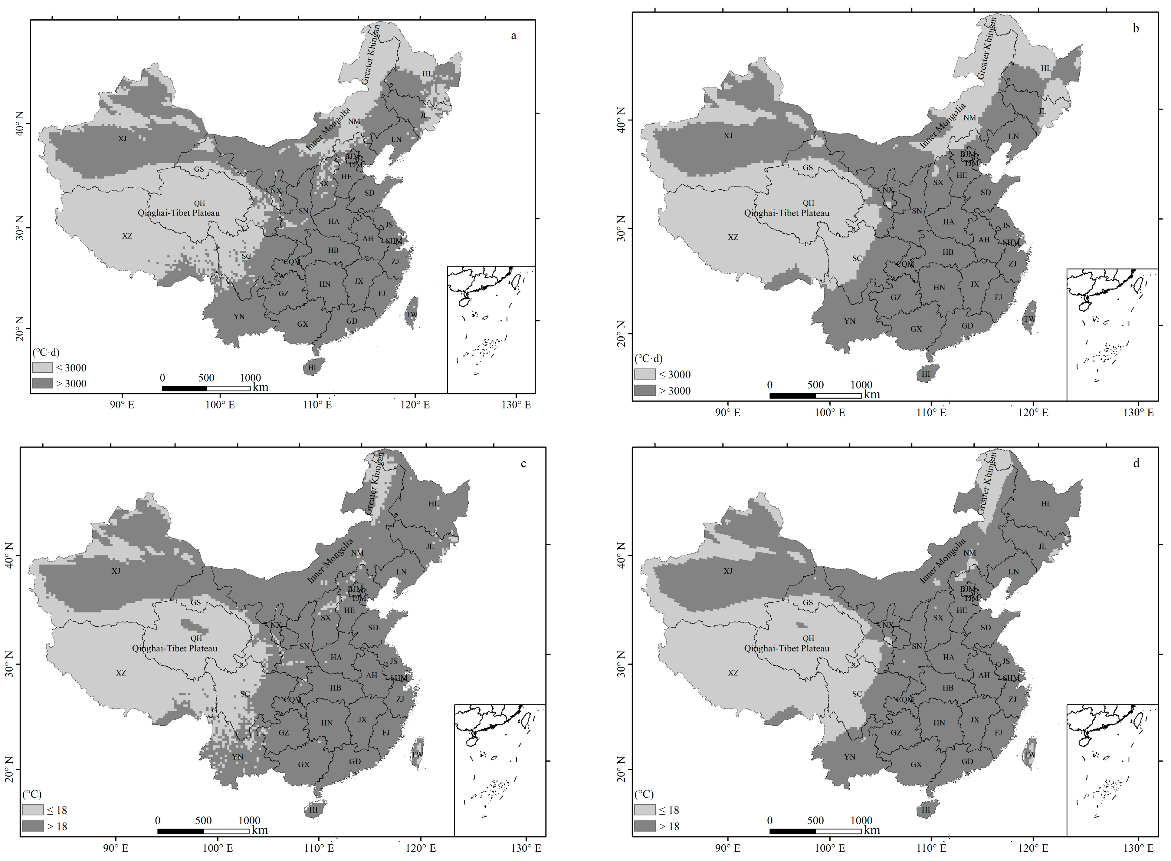
It can be observed that the zonality of the accT0 distribution was evident across the country (Figure 1). accT0 progressively expanded from north to south, particularly in the east, creating optimal temperature conditions and a beneficial environment for the growth and development of various crops. Due to the high proportion of land and chilly environment, accT0 in the Qinghai–Tibet Plateau was usually lower than that in other parts of the country. When its composition was predominantly influenced by topography, which affected the zonality of the climate along the latitude, a pleasant temperate continental plateau climate was formed. accT0 of the southeast slope of the plateau (Southern Tibet, Southeast Tibet Valley) was higher, exceeding 3000 °C∙d. Most parts of northeast China had a low accT0, generally around 3000 °C, which was suitable for cultivating chimonophilous and cold-tolerant crops.

The geographical distribution of Th is also illustrated in Figure 1. The Tibetan plateau had the lowest Th in the country. Th frequently fell below 12 °C in the Tibetan plateau and alpine regions, and in some parts of the plateau, Th even dropped below 6 °C, preventing crops from being sown. Other plateau regions, where Th values were essentially below 18 °C, can be seeded with cold-tolerant crops such as spring wheat and fodder. Due to high latitude or altitude, the mountains at the northern end of Greater Khingan and many other high-alpine areas had a Th below 18 °C. In other parts of China, Th was well above 18 °C, allowing most crops to flourish. The accT0 and Th distribution maps also indicated a unique dark zone in the northeast of the Qinghai–Tibet Plateau, where heat was higher than that in other regions, as previously noted [31]. The spatial distribution of mean annual precipitation was also shown in Figure 1. The overall mean annual precipitation showed a steady downward trend from southeast to northwest.

3.2. Evaluation of Simulation Results

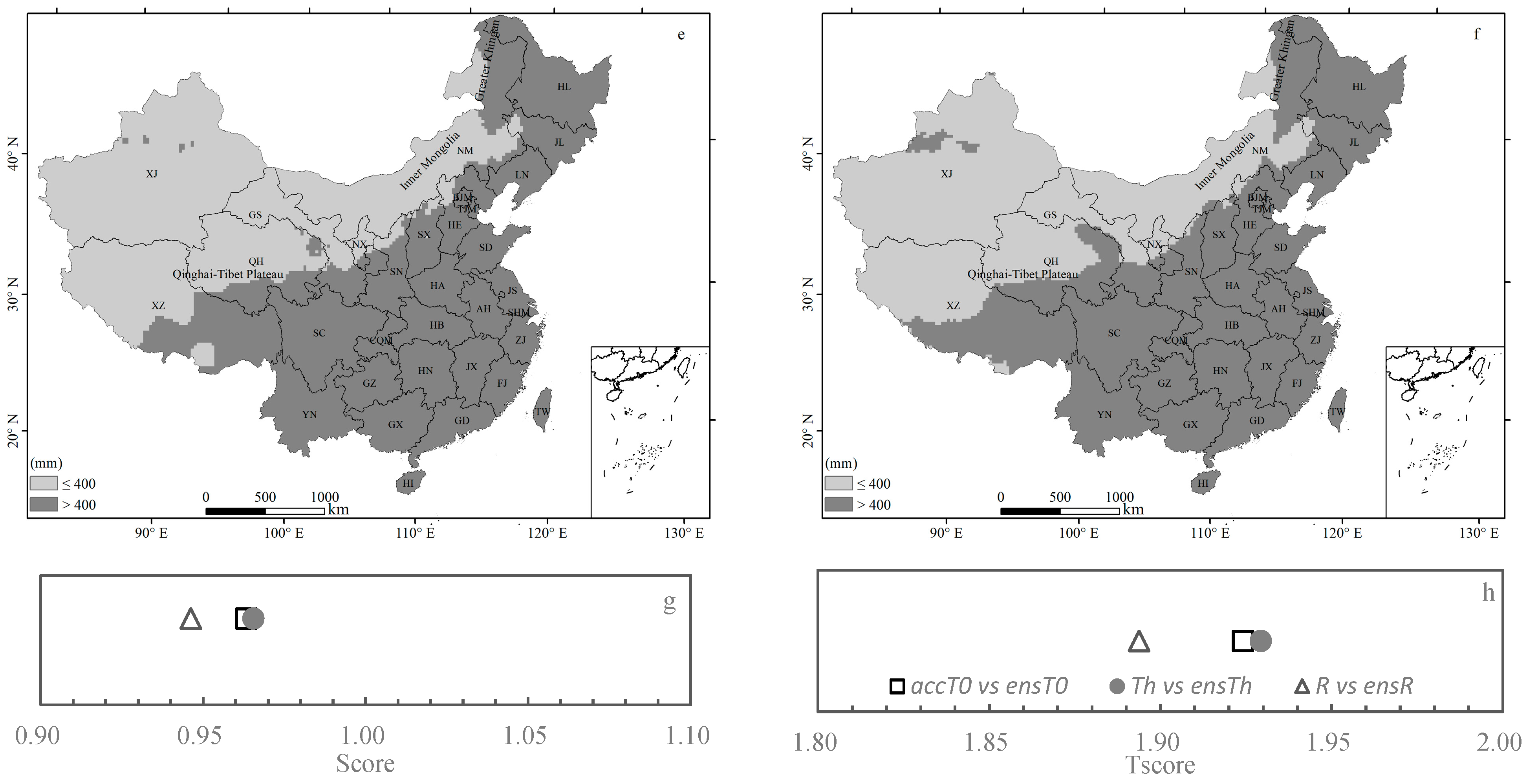
Using the main indices in Table 1 as a guide, the distribution of accumulated temperature, the hottest July temperature, and the annual precipitation between observed data and simulated data in China in the reference period are depicted in Figure 2. These three sets of data revealed that the spatial distribution of simulated data and observed data was comparable for each indicator. The accumulated temperature (accT0 and ensT0, <3000 °C·d) and in the hottest monthly temperature (Th and ensTh, <18 °C) were the lowest in the Qinghai–Tibet Plateau and Northeast China, while annual precipitation ranges (R and ensR, <400 mm) were the lowest in Northwest China and Inner Mongolia. Intriguingly, a region of light color appeared to the northeast of the plateau, indicating that the accumulated and average temperatures there were higher than 3000 °C and 18 °C. Both are represented in the figures for the observation and simulation results, but the simulated range was narrower than the observed range. The observational and simulated data nevertheless differed in some other ways. For instance, the boundary line of 18 °C in the simulated data was clear and smoother, but the observed data of accT0 and Th showed that there were many scattered distributions on the different terrains across the southwest region. The precipitation elements in central China and parts of Xinjiang (XJ) both exceeded 400 mm; however, the observed range was much smaller than the simulated range (Figure 2e,f). Although the regional distribution of the simulated and observed data was largely comparable, the specific performance outcomes were slightly different.

The scores and Taylor scores between various observation and ensemble data are also shown in Figure 2. According to statistical indices, the spatial correlation coefficient between the simulation and observation data was 0.95~0.97, in which Th, accT0, and R showed a strong spatial correlation. The simulation effects of spatial distribution and numerical values can be fully modeled by Taylor scores. Based on accT0, Th, and R, simulation scores (1.89 to 1.93) were rather good. The results showed that ensT0, ensTh, and ensR essentially mimicked the observational properties of the relevant annual climate elements.

3.3. Changes of the Agroclimatic Regions under the Historical Conditions

The distribution of agroclimatic regions in period I and the boundary changes of agroclimatic regions in period II, period III, and period IV are shown in Figure 3. The green, yellow, and blue polygons represent the distribution of the EMR, the NAR, and the THCR, respectively. The THCR was mainly distributed in Tibet Autonomous Region (XZ), southern Xinjiang (XJ), Qinghai (QH), most of Gansu (GS), southwest Ningxia Hui Autonomous Region (NX), western Sichuan (SC), and northwest Yunan (YN). The NAR included most of Xinjiang (XJ), most of Gansu (GS), north-central Ningxia Hui Autonomous Region (NX), most of Inner Mongolia (NM), western Jilin [32], and a small portion of Shaanxi (SN) and Shanxi (SX) bordering Inner Mongolia. The EMR was the southeastern China excluding the THCR and NAR (Figure 3a).

Using 1961–1991 (period I) as a base period, we compared the spatial changes in agroclimatic regions in three periods. From the changes in the agroclimatic regions, there was no significant change in the THCR between period II and period I. From period III, the northeast corner of the THCR shifted significantly to the southwest. In period Ⅳ, the northeast corner continued to be shifted towards the southwest, with a total displacement of about 170 km, leading to the withdrawal of the THCR from the southwest of Ningxia Hui Autonomous Region (NX) and east Gansu (GS) (Figure 2b–d).

Compared to period I, the boundary between the NAR and the EMR in eastern Jilin [32] in period II contracted southward, with a maximum of about 100 km. The boundary between Shaanxi (SN) and Ningxia (NX) in the middle section moved southward, increasing the range of the NAR in this section. There was no significant change in the boundaries of Xinjiang (XJ) and Gansu (GS) regions in the western section. In period III, the northern boundary of the NAR slightly shifted eastward, while the eastern boundary expanded eastward and northward. During this period, due to the southwest displacement in the northeast of the THCR, the central boundary of the NAR extended westward. The middle part of the boundary remained unchanged compared to that in the previous period. The boundary changes at period III were consistent with the analysis results of Li [7] in terms of the agricultural pastoral ecotone based on precipitation. During period IV, the north boundary moved eastward, and the eastern boundary of the NAR slightly moved southward, while the middle boundary moved northward. However, compared to period I, the north boundary moved eastward, and the eastern boundary of the NAR lifted to the north and expanded to the east. At the same time, the central boundary lifted northward and extended westward. Compared to the change in agroclimatic regions in the past 60 years, the most significant changes were in the northeastern part of the THCR, and the central and northeastern parts of the NAR. From the perspective of area change, the THCR area was continuously decreasing. By period IV, compared with period I, the area decreased by about 4.8 × 10⁴ km². The area of the EMR and the NAR alternatively increased or decreased. In the period II and period III, the area in the NAR continued to rise, but decreased in period IV. The change in the EMR area was the opposite. Compared to period I, the NAR area in period IV increased by about 6.7 × 10⁴ km², and the EMR lost 1.8 × 10⁴ km². However, generally, the EMR was the largest region in China, followed by THCR and the NAR.

The changes in agroclimatic regions indicated changes in heat and precipitation. Representative stations in the areas with significant boundary changes are marked in Figure 3, and detailed information is provided in

Table 2. Changes in thermal and precipitation resources around the northern boundary of the THCR and NAR.

Num	Station	Province	accT0/°C·d					Th/°C
			Period I	Period II	Period III	Period IV	Variation	Period I	Period II	Period III	Period IV	Variation
1	Yuzhong (Yz)	GS	3055.1	3064.9	3135.5	3233.4	178.3	18.8	18.9	19.3	19.5	0.7
2	Anding (An)	GS	2972.1	3035.0	3173.3	3307.4	335.2	18.3	18.6	19.3	19.7	1.4
3	Huajialing (Hj)	GS	2132.1	2174.3	2237.8	2323.6	191.5	14.6	14.8	15.1	15.4	0.8
4	Xiji (Xj)	NX	2730.7	2771.3	2851.2	2959.9	229.2	17.7	18.0	18.3	18.7	1
5	Longde (Ld)	NX	2612.2	2643.9	2710.1	2822.1	228.8	16.8	17.0	17.3	17.7	0.9
			R/mm					α
			Period I	Period II	Period III	Period IV	Variation	Period I	Period II	Period III	Period IV	Variation
6	Tongyu (Ty)	JL	406.0	391.4	370.7	364.3	−41.7	0.06	−0.09	−0.29	−0.38	−0.45
7	Bayaertu (By)	NM	430.4	437.8	411.2	401.0	−29.4	0.31	0.31	0.08	0.01	−0.30
8	Duolun (Dl)	NM	370.1	386.5	377.9	383.7	13.6	−0.43	−0.19	−0.33	−0.25	0.17
9	Zhangjiakou (Zj)	HB	398.5	403.6	388.7	411.1	12.6	−0.02	0.04	−0.13	0.13	0.15
10	Huailai (Hl)	HB	383.1	372.4	367.9	397.1	14.0	−0.20	−0.37	−0.44	−0.03	0.17

GS: Gansu Province. NX: Ningxia Hui Autonomous Region. JL: Jilin Province. NM: Inner Mongolia. HB: Hebei Province. Variation represents the difference in elements between period IV and period I.

. Meteorological stations 1 to station 5 were selected from areas with a significant change in the northeast boundary of the THCR: Yuzhong, Anding, and Huajialing in Gansu Province (GS), and Xiji and Longde in Ningxia Hui Autonomous Region (NX). Over the past 60 years, there has been a significant increase in accT0 and Th at the five stations. Compared to period I, the average accT0 and Th of the five stations in period IV increased by 228.8 °C·d and 0.9 °C, respectively. For station 2, with the most significant heat change, accT0 increased from 2972.1 to 3307.4 °C·d, and Th increased from 18.3 to 19.7 °C, exceeding the average of the five stations. There were varying degrees of changes in the boundary between the NAR and the EMR, with the most significant change occurring during period Ⅳ. The 400 mm precipitation was the dominant indicator in this region, indicating that there was a significant change in precipitation in the past 30 years. Statistics showed that from 1961–1990 to 1991–2020, there were two periods of changes in precipitation resources in the NAR (Table 2). From Figure 3, the boundary between the east and central regions of the NAR was clearly shifting northward. Station 6 and station 7 were two meteorological stations near the east boundary, while stations 8 to 10i were three stations near the center boundary. The annual accumulated frequency of precipitation decreases with a decreasing standardization coefficient, α, in accordance with the relationship between precipitation and the standardization coefficient, α [26]. The standardization coefficient of precipitation drastically reduced along with the precipitation in station 6 and station 7, as seen in Table 2. α in station 7 dropped from 0.31 to 0.01, while α in station 6 declined from a positive value in period I to a negative value in period IV. The fluctuation of precipitation and the precipitation standardization coefficient, α, increased in stations 8 10, with α at station 9 increasing from negative (period I) to positive (period IV), indicating an increase in the accumulated frequency of precipitation at all three stations. These were also the reasons why the line between the NAR and the EMR lifted to north in the middle.

3.4. Changes in Agroclimatic Regions under the Future Climate Scenarios

According to the indices and standards for agroclimatic regions (Table 1), the distribution of agroclimatic regions from 1981 to 2005 (the contemporary period, period Iens) and under different climate scenarios was divided (Figure 4). During period Iens, the THCR was mainly distributed in Tibet Autonomous Region, Qinghai, southern Xinjiang, most of Gansu, western Sichuan, and northwest Yunan. The NAR included Xinjiang, most of Gansu, north central Ningxia Hui Autonomous Region, most of Inner Mongolia, and southwest Jilin. The EMR was the southeastern China excluding the THCR and NAR. Compared to the period Iens, under RCP2.6, the northeast corner of the THCR boundary slightly retreated during the period IIens. The range of the THCR slightly changed comparing that in period IIIens with that in IIens. The boundary between the NAR the EMR underwent varying changes. In the period IIens, the central boundary between northeastern Shanxi and southwest Hebei rose northward. The northern and eastern boundary expanded outward. In the period IIIens, the northern boundary moved westward slightly, and the eastern boundary shrunk southward and westward. The central boundary moved slightly north. The range of changes in the THCR under the RCP4.5 scenario was comparable to that under the RCP2.6 scenario. Compared to period Iens, the scope of the THCR continued to shrink, the range of the boundary changed between the NAR, and the EMR increased. The central boundary moved northward slightly in the period IIens. The boundary in the north and middle moved westward and northward, respectively, during the period IIIens. Moreover, the northward movement of the central boundary was greater than that of the same period under the RCP2.6 scenario. Under the RCP8.5 scenario, the range of the THCR was reduced during the period IIens and period IIIens, similar to that under RCP4.5 and RCP2.6. In the period IIens, the eastern boundary showed a southward displacement, while in the period IIIens the eastern boundary continued to shrink. In addition, the middle boundary between shanxi and Hebei was lifted northward.

From the perspective of area change, the THCR area was reduced. By the period IIIens, the area of the THCR decreased the most under the RCP8.5 scenario (by 7.8 × 10⁴ km²), followed by that in the RCP4.5 and RCP2.6 scenarios. Similarly to the THCR, the area of the NAR decreased by 5.0 × 10⁴ km², 3.7 × 10⁴ km², and 7.3 × 10⁴ km² by the end of period IIIens under the three climatic scenarios, respectively. The EMR area had been increasing under the three climatic scenarios, with an increase of 9.3 × 10⁴ km², 9.5 × 10⁴ km², and 1.5 × 10⁵ km² by the end of the period IIIens, respectively. Although there were slight changes in the spatial distribution and area of agroclimatic regions under different scenarios, there was not much of a change in the proportion of the area. The changes in the proportion of agroclimatic region areas under different scenarios are shown in Figure 5. Although the northeast boundary of the THCR slightly retreated, due to the small reduction in area, the proportion of the THCR area in RCP2.6 and RCP4.5 remained unchanged at 27%. Under RCP8.5, the area decreased to 26% by the period IIIens. The proportion of the NAR and EMR areas showed different changes in three scenarios. The NAR area accounted for 26% in the period Iens. During the IIens period, it decreased by 1% to 25% and remained unchanged thereafter. Under the RCP2.6 and RCP4.5 scenarios, the proportion of the EMR area showed consistent changes, with an increase of 1% to 47% in the period IIens, and remained unchanged thereafter. However, under the RCP8.5 scenario, the EMR area had been continuously increasing, increasing to 48% during the period IIens and to 49% during the period IIIens. Overall, under the RCP2.6 and RCP4.5 scenarios, the changes in the area of agroclimatic regions were consistent, with a significant increase or decrease in the period IIens compared to those in the period Iens, and then remained unchanged. In the RCP8.5 scenario, the EMR continued to increase, while the THCR began to decrease in the period IIIens.

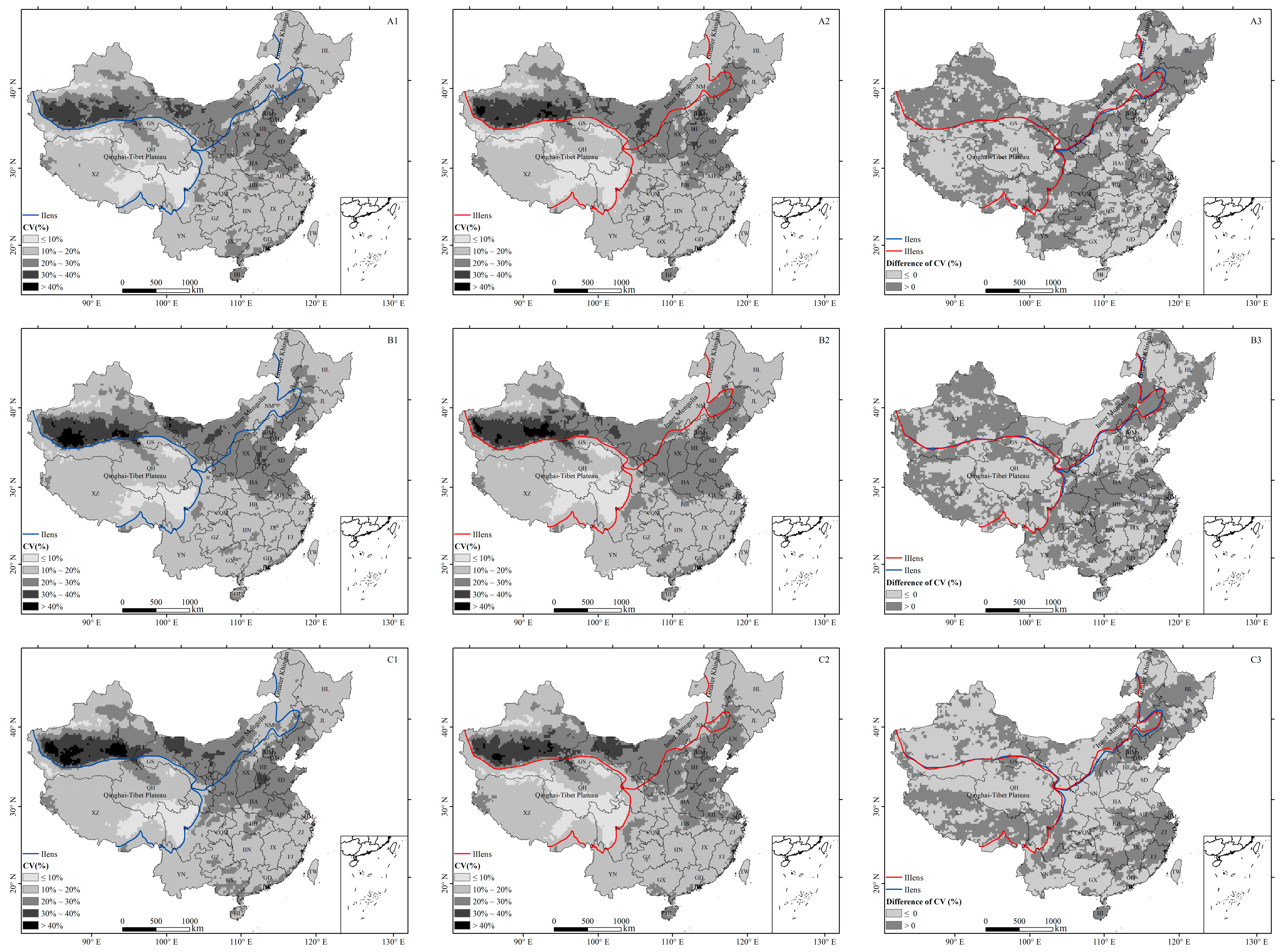
In the context of future climatic scenarios, the extent of the THCR and the NAR may be decreased. However, the scope of the EMR may be likely to expand, suggesting that the expanded land would be well suited to expanding agricultural production. Let us examine the evolution of the precipitation. The coefficient of variation (CV) in precipitation in climatic scenarios revealed large inter-annual fluctuations (Figure 6). The CV values in the central and western parts of the NAR and the central parts of the EMR were both above 0.2, while other regions typically had a CV below 0.2. In the northeast part of the THCR and in the eastern and central parts of the NAR, the regions could fluctuate greatly, with a CV typically ranging from 0.1 to 0.3. The eastern and center portions of the NAR and the northeast portion of the THCR would have an increase in CV compared to that in the period IIens under the RCP2.6 scenario. In the central parts of the NAR, the CV would decline under the RCP4.5 scenario. Additionally, the CV in the northeast of the THCR would decline under the RCP8.5 scenario. This shows that the CV would be more profound and exhibit larger oscillations in regions where the agroclimatic regions changed under various climatic scenarios.

4. Discussion

4.1. Indices and Standards of the Agroclimatic Regions

There were similarities and significance in the indices of agroclimatic regionalization, which accorded with the principles of agricultural production design. The lower limit of optimum heat during the ripening season for middle rice or late-maturing maize was determined by a cumulative temperature of 3000 °C·d. Regions with an accumulated temperature below 3000 °C·d generally relied on cool and cold-resistant crop varieties, making animal husbandry the primary industry in these areas [1]. Forest development required a minimum amount of rainfall of 400 mm. These indices, along with an elevation index of 3000 m above sea level in the eastern part of the Qinghai–Tibet Plateau and an average temperature index of 18 °C in the hottest month, served as key indices for dividing agroclimatic regions. This index system held significant guiding value for China’s agroclimatic regionalization. The second national agroclimatic regionalization and several similar agroclimatic regionalizations incorporated findings from numerous researchers [1,7,9]. However, the index system overlooked the features of the environment, particularly those that may be raised in future scenarios, since it relied solely on static geographical and climatic parameters. According to studies conducted in Poland [14], Canada [15,16], and other continents [17,18], significant changes were observed in agroclimatic indices related to crop growth due to climate change, such as alternations in growing season length as well as shifts in its beginning and end dates. In addition to traditional agroclimatic factor index methods, introducing new mathematical and statistical methods is also crucial, such as remote sensing technology. Remote sensing technology can provide comprehensive quantitative positioning information with strong timeliness, high accuracy, and a wide monitoring range, helping to update agricultural climate zoning data and ensure their practicality in a timely manner [33].

4.2. Distribution and Changes in the Agroclimatic Regions

Due to its location in southwest China, the principal determinants of the THCR’s range were accumulated heat and elevation. The northeastern boundary gradually shifted southwestward between 1961 and 2020. Changes in precipitation resulted in an expansion of the NAR in northern China, consequently leading to a comparable drop in the EMR (Figure 3). Temperature and precipitation observations from neighboring meteorological stations indicated alternations in boundaries (Table 2). These findings supported previous findings [7,9], which illustrated how China’s agroclimatic regions were transforming due to climate change. Additionally, the rate of the THCR declined when the temperature warmed after the 1990s [34]. In the future climatic scenarios, although limited, the northeastern corner of the THCR will shift southwestward while the NAR distribution will decrease. The EMR will expand its coverage and scope. In comparison to the RCP2.6 and RCP4.5 scenarios, the RCP8.5 scenario greatly amplified variations within each region. The reduction extent of the THCR was constrained by topography and altitude; hence, the NAR and EMR will continue to grow or change accordingly. While little change occurred on either side of the boundary, height limited the eastern boundary of the THCR, whereas the alpine terrain affected its northern boundary—both contributing factors to potential regional changes observed via the considerable internal warming detected and modeled within the THCR (Figure 2 and Figure 3), consistent with other researchers’ findings [31,34]. Climate change would increase areas of the EMR and increase the possibility of the northern boundary of crop cultivation shifting northward in the future [20], but the large variability in precipitation in the displacement areas would also bring uncertainty to the northward migration of crop cultivation.

4.3. Uncertainty

The altitude of the eastern part of the plateau at 3000 m above sea level served as a reference index for the geographic limitations of the distribution of the THCR. However, with the accumulative temperature and the average temperature of the hottest month as indices, the THCR range in the east will be bigger than that indicated by altitude alone as an index. It is important to note that due to climate change and rising temperatures, there may be a gradual expansion rather than a contraction of the THCR range. Consequently, other agroclimatic regions will also experience changes in size and scope. Additionally, in areas with complex terrain and significant elevation variations, regional boundaries during the process of regionalization may appear uneven or result in several isolated island-like areas outside designated regions. To ensure smoothness and continuity within these regions, adjustments such as increased smoothness or the elimination of isolated islands might be necessary; however, this could lead to some local data loss. To perform the spatial interpolation of accumulative temperature and average temperature components, we employed the expert interpolation software ANUSPLIN 4.2, an expert interpolation software tool specifically designed for time series data [35,36]. ANUSPLN proves suitable for enhancing interpolation accuracy while reflecting relationships between the meteorological variables and their impacted components. Previous studies [37,38] have shown its effectiveness in spatially interpolating cumulative temperature and related elements across complex terrains like those found in the southeast corner of the Tibetan Plateau or Daba Mountains within the Qinling Mountain region. Despite ANUSPLIN’s high accuracy in temperature interpolation overall, it should be noted that uncertainty remained particularly pronounced when interpolating hilly areas with inadequate sampling coverage [35]. Additionally, ANUSPLIN interpolation data showed a trend of underestimation, especially at a high altitude where the underestimation intensity was very significant [37]. The use of climate models to assess and predict the characteristics of climate change can provide a scientific basis for adjusting agricultural layout to adapt to climate change. However, uncertainties existed in climate predictions and estimates due to uncertainty in future scenarios, uncertainties in natural variability within the climate system, and uncertainties in characterizing climate processes [39,40,41].

5. Conclusions

The agroclimatic regions in China experienced notable changes from 1961 to 2020 under climate change. Regional climate models were utilized for predicting climatic characteristics and analyzing the spatial distribution of the agroclimatic regions under the low-, middle-, and high-emission scenarios relative to those in the reference period (1981–2005).

The historical change analysis of agroclimatic regions showed that the spatial variation in the THCR was most obvious. The northeast corner of the THCR contracted towards the southwest by 1991–2020, retreating from the southwest of Ningxia (NX) and eastern Gansu (GS) with a spatial displacement of about 170 km. The range of the NAR was predominantly located in northern China under the influence of annual precipitation control. Over the past 60 years, boundaries of the NAR underwent significant changes with a shift eastward at its northern boundary, expansion outward at its northeastern boundary, and a northward rise at its central boundary. The EMR area decreased due to the changes in the range and area of the THCR and the NAR.

The spatial distribution and area of agroclimatic regions in China will inevitably change under the future climate scenarios. By 2060, the northeastern corner of the THCR will have moved further southwest and be narrower than it was during the reference period. The THCR area accounted for 26% of China’s total area under the RCP8.5 scenario, decreasing by 1%, while 27% of the area remained stable under the RCP4.5 and RCP2.6 scenarios. The eastern boundaries of the NAR will shrink to the south or east, while its central boundaries will rise to the north. The proportion of area changes was similar in all three scenarios, resulting in a 1% decrease in area (26% for the reference period). The scope of the EMR will expand, and so will the field. The area will cover 48% of China’s land under the RCP2.6 and RCP4.5 scenarios, an increase of 1%, while in the RCP8.5 scenario, it would be 49%, an increase of 2%. The precipitation coefficients of variation in the central EMR and western NAR will be considerable, with noticeable fluctuations in areas where the boundaries of the agroclimatic region change. This suggests that future climate change will have a considerable influence on the border area close to agroclimatic boundaries, increasing the risk of agricultural production in these areas.

References

1. Li, S. Agroclimatic regionalization of China. J. Nat. Resour. 1987, 2, 71–82. [Google Scholar]
2. IPCC. Climate Change 2007: Synthesis Report; Cambridge University Press: Cambridge, MA, USA, 2007. [Google Scholar]
3. Chu, Z.; Guo, J.; Zhao, J. Impacts of future climate change on agroclimatic resources in Northeast China. J. Geogr. Sci. 2017, 27, 1044–1058. [Google Scholar] [CrossRef]
4. Piticar, A. Changes in agro-climatic indices related to temperature in Central Chile. Int. J. Biometeorol. 2019, 63, 499–510. [Google Scholar] [CrossRef] [PubMed]
5. Trnka, M.; Eitzinger, J.; Semerádová, D.; Hlavinka, P.; Balek, J.; Dubrovský, M.; Kubu, G.; Štěpánek, P.; Thaler, S.; Možný, M.; et al. Expected changes in agroclimatic conditions in Central Europe. Clim. Chang. 2011, 108, 261–289. [Google Scholar] [CrossRef]
6. Vasconcelos, R.d.L.; Rocha, L.A.G.; de Sousa, R.L.; Ferrari, J.M.d.S.; Lima, R.d.S.; Garcia, A.; Filho, L.R.A.G.; Gabriel, C.P.C. Agroclimatic Zoning for the Palm Euterpe edulis M. in So Paulo State, Brazil. J. Agric. Sci. 2019, 11, 217–230. [Google Scholar]
7. Li, Q.; Pan, X. The impact of climate change on boundary shift of farming pasture ecotone in northern China. J. Arid Land Resour. Environ. 2012, 26, 1–6. [Google Scholar]
8. Tian, Z.; Yang, X.; Sun, L.; Fischer, G.; Liang, Z.; Pan, J. Agroclimatic conditions in China under climate change scenarios projected from regional climate models. Int. J. Climatol. 2013, 34, 2988–3000. [Google Scholar] [CrossRef]
9. Liao, Y.M.; Zhai, P.M. Study on China’s Oning and Climate Atlas Scheme; China Meteorological Press: Beijing, China, 2014. [Google Scholar]
10. Nabati, J.; Nezami, A.; Neamatollahi, E.; Akbari, M. GIS-based agro-ecological zoning for crop suitability using fuzzy inference system in semi-arid regions. Ecol. Indic. 2020, 117, 106646. [Google Scholar] [CrossRef]
11. Wu, D.R.; Wang, P.J.; Huo, Z.G.; Yuan, X.K.; Jiang, H.F.; Yang, J.Y.; Ma, Y.P.; Guo, S.L. Climatic suitability regionalization of Camellia oleifera Abel. in China. Chin. J. Ecol. 2021, 40, 1313–1323. [Google Scholar]
12. Zuo, C.; Song, F.; Shi, Y.; Luo, D. Climate regionalization of hybrid hazel planting in Xinjiang. Chin. J. Agrometeorol. 2020, 41, 146–155. [Google Scholar]
13. Zhong, X.L.; Wang, D.L.; Zhao, P. Frost-driven agricultural climatic division of winter wheat in Huang-huai wheat produciton zones. Chin. J. Eco-Agric. 2008, 16, 11–15. [Google Scholar] [CrossRef]
14. Graczyk, D.; Kundzewicz, Z.W. Changes of temperature-related agroclimatic indices in Poland. Theor. Appl. Climatol. 2016, 124, 401–410. [Google Scholar] [CrossRef]
15. Chipanshi, A.; Berry, M.; Zhang, Y.; Qian, B.; Steier, G. Agroclimatic indices across the Canadian Prairies under a changing climate and their implications for agriculture. Int. J. Climatol. 2021, 42, 2351–2367. [Google Scholar] [CrossRef]
16. Qian, B.; De Jong, R.; Gameda, S.; Huffman, T.; Neilsen, D.; Desjardins, R.; Wang, H.; McConkey, B. Impact of climate change scenarios on Canadian agroclimatic indices. Can. J. Soil Sci. 2013, 93, 243–259. [Google Scholar] [CrossRef]
17. Linderholm, H.W.; Walther, A.; Chen, D. Twentieth-century trends in the thermal growing season in the Greater Baltic Area. Clim. Chang. 2008, 87, 405–419. [Google Scholar] [CrossRef]
18. Liu, J.; Zhai, P. Changes in climate regionalization indices in China during 1961–2010. Adv. Atmos. Sci. 2014, 31, 11. [Google Scholar]
19. Ding, Y. National assessment report of climate change (I): Climate change in China and its future trend. Adv. Clim. Chang. Res. 2006, 2, 3–8. [Google Scholar]
20. Yang, X.; Liu, Z.; Chen, F. The possible effects of global warming on cropping systems in China VI.possible effects of future climate change on northern limits of cropping system in China. Sci. Agric. Sin. 2011, 44, 1562–1570. [Google Scholar]
21. Shi, G.; Ye, P.; Yang, X. Spatio-Temporal Variation Analysis of the Biological Boundary Temperature Index Based on Accumulated Temperature: A Case Study of the Yangtze River Basin. Int. J. Geo-Inf. 2021, 10, 675. [Google Scholar] [CrossRef]
22. Hutchinson, M.F. Interpolation of rainfall data with thin plate smoothing splines—Part I: Two dimensional smoothing of data with short range correlation. J. Geogr. Inf. Decis. Anal. 1998, 2, 139–151. [Google Scholar]
23. Han, Z.; Xu, Y.; Wu, J.; Shi, Y. Evaluation on the simulated runoff in China and future change projection based on multiple regional climate models. Clim. Chang. Res. 2022, 18, 305–318. [Google Scholar]
24. Tong, Y.; Han, Z.; Gao, X. Bias correction in climate extremes over China for high-resolution climate change RegCM4 simulations using QM and QDM methods. Clim. Environ. Res. 2022, 27, 383–396. [Google Scholar]
25. IPCC. Climate Change 2013: The Physical Science Basis; Cambridge University Press: Cambridge, MA, USA, 2013. [Google Scholar]
26. Chen, W. Theoretical calculation of the guarantee rate of agricultural climate indicators. Tibet J. Agric. Sci. 1979, 4, 21–28. [Google Scholar]
27. Taylor, K.E. Summarizing multiple aspects of model performance in a single diagram. J. Geophys. Res. Atmos. 2001, 106, 7183–7192. [Google Scholar] [CrossRef]
28. Qiu, B.; Lu, Q. A tentative regionalization of agroclimate of China. Acta Geogr. Sin. 1980, 35, 116–125. [Google Scholar]
29. Qiu, B. A new discussion of the regionalization of agroclimate in China. Acta Geogr. Sin. 1986, 41, 202–209. [Google Scholar]
30. Zhen, J.; Yin, Y.; Li, B. A new scheme for climate regionalization in China. Acta Geogr. Sin. 2010, 65, 3–12. [Google Scholar]
31. Li, C.; Kang, S. Review of studies in climate change over the Tibetan Plateau. Acta Geogr. Sin. 2006, 61, 327–335. [Google Scholar]
32. Bazi, Y.; Alajlan, N.; Melgani, F.; AlHichri, H.; Malek, S.; Yager, R.R. Differential evolution extreme learning machine for the classification of hyperspectral images. IEEE Geosci. Remote Sens. Lett. 2014, 11, 1066–1070. [Google Scholar] [CrossRef]
33. Terehov, A.G.; Muratova, N.R.; Arkhipkin, O.P.; Spivak, L.F. Agroclimatic zoning of Kazakhstan territory using remote sensing data. In Proceedings of the IEEE International Geoscience & Remote Sensing Symposium, Honolulu, HI, USA, 24–28 July 2000; pp. 1975–1977. [Google Scholar]
34. Zhao, J.; Hu, J.; Guo, X.; Wang, Q.; Wang, L.; Wang, M. Variation characteristics of thermal resources in Qinghai-Tibet Plateau in recent 50 years. Chin. J. Appl. Environ. Biol. 2022, 28, 822–828. [Google Scholar]
35. Hijmans, R.J.; Cameron, S.E.; Parra, J.L.; Jones, P.G.; Jarvis, A. Very high resolution interpolated climate surfaces for global land areas. Int. J. Climatol. 2005, 25, 1965–1978. [Google Scholar] [CrossRef]
36. Liu, Z.; McVicar, T.R.; Li, L. Interpolation for time series of meteorological variables using ANUSPLIN. J. Northwest A&F Univ. (Nat. Sci. Ed.) 2008, 36, 227–234. [Google Scholar]
37. Tan, J.; Li, A.; Lei, G. Contrast on Anusplin and Cokriging meteorological spatial interpolation in southeastern margin of Qinghai-Xizang Plateau. Plateau Meteorol. 2016, 35, 875–886. [Google Scholar]
38. Zhang, S.; Bai, M.H.; Qi, G.; Liang, J.; Zhao, T. Spatial simulation of active accumulative temperature ≥10 °C in Qinling-Daba Mountains based on Anusplin and multiple linear regression model. Res. Soil Water Conserv. 2022, 29, 184–196. [Google Scholar]
39. Gillingham, K.; Nordhaus, W.D.; Anthoff, D.; Blanford, G.; Bosetti, V.; Christensen, P.; McJeon, H.; Reilly, J.; Sztorc, P. Modeling Uncertainty in Climate Change: A Multi-Model Comparison; MIT Joint Program on the Science and Policy of Global Change: Cambridge, MA, USA, 2015. [Google Scholar]
40. Duan, Q.; Xia, J.; Miao, C.; Sun, Q. The uncertainty in climate change projections by global climate models. Chin. J. Nat. 2016, 38, 182–188. [Google Scholar]
41. Tao, F.; Rötter, R.P.; Palosuo, T.; Díaz-Ambrona, C.G.H.; Schulman, A.H. Contribution of crop model structure, parameters and climate projections to uncertainty in climate change impact assessments. Glob. Chang. Biol. 2017, 24, 1291–1307. [Google Scholar] [CrossRef]
Figure 1. Spatial distribution of main climatic indices in agroclimatic regionalization in China from 1961 to 2020 ((a) is the distribution of accT0. (b) is the distribution of Th. (c) is distribution of R).
Agronomy 14 00293 g001
Figure 2. Predominant climate indicators of observation data and simulation results over 1981–2005 ((a) accT0, (b) ensT0, (c) Th, (d) ensTh; (e) R, and (f) ensR), and the SCORE (g) and Taylor score among different data (h).
Agronomy 14 00293 g002aAgronomy 14 00293 g002b
Figure 3. Geographical displacement of agroclimatic region boundaries in different periods. (The yellow, blue, and green polygon surfaces represent the NAR, THCR and EMR, respectively, in period I. (a) The distribution of agroclimatic regions. (bd) The displacement of agroclimatic region boundaries in periods II to IV, where saffron lines are the boundaries of the three regions in period II, dark blue lines are the boundaries of the three regions in period III, and red lines, similarly, are the boundaries of the three agroclimatic regions in period IV. Black dots are representative meteorological stations, as shown in Table 2.
Agronomy 14 00293 g003
Figure 4. Geographical displacement of agroclimatic region in 1981–2005 and the boundary lines at different periods under future climatic scenarios. (The yellow, blue, and green polygon surface represent the NAR, THCR, and EMR, respectively, in the period Iens. The dark blue and red lines are the boundary lines of the agroclimatic regions during the periods IIens to IIIens. (a) The RCP2.6 scenario. (b) The RCP4.5 scenario. (c) The RCP8.5 scenario.
Agronomy 14 00293 g004
Figure 5. The area variation in the NAR, THCR, and EMR during the different periods under the future climatic scenarios (the yellow, blue, and green polygon surfaces represent the NAR, THCR, and EMR, respectively. (a) The RCP2.6 scenario. (b) The RCP4.5 scenario, (c) The RCP8.5 scenario).
Agronomy 14 00293 g005
Figure 6. Variation coefficient of annual precipitation under different climate scenarios during two periods (A1A3) under the RCP2.6 scenario, (B1B3) under the RCP4.5 scenario, and (C1C3) under the RCP8.5 scenario. The dark blue and red lines are the boundary lines of the EMR, the NAR, and the THCR during the periods IIens to IIIens. The difference in CV is the CV in the period IIIens minus the CV in the period IIens.
Agronomy 14 00293 g006