
Design of an Autonomous Orchard Navigation System Based on Multi-Sensor Fusion


 ,
,
Abstract
1. Introduction
2. Materials and Methods
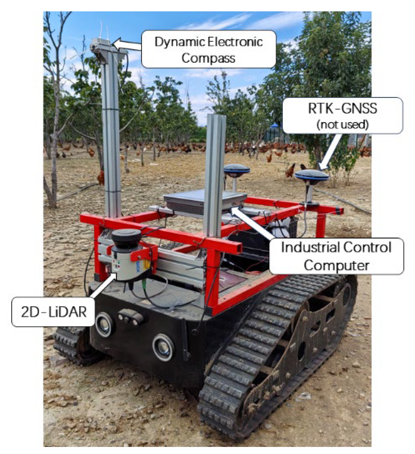
2.1. System Hardware Components
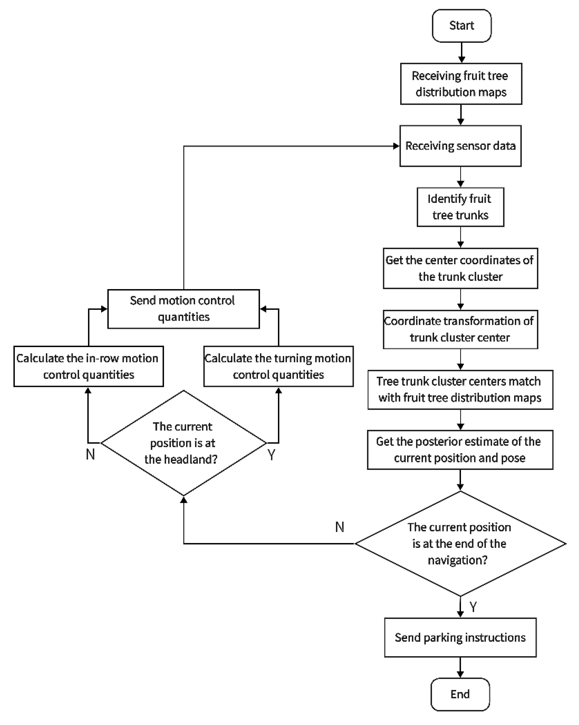
2.2. System Software Implementation
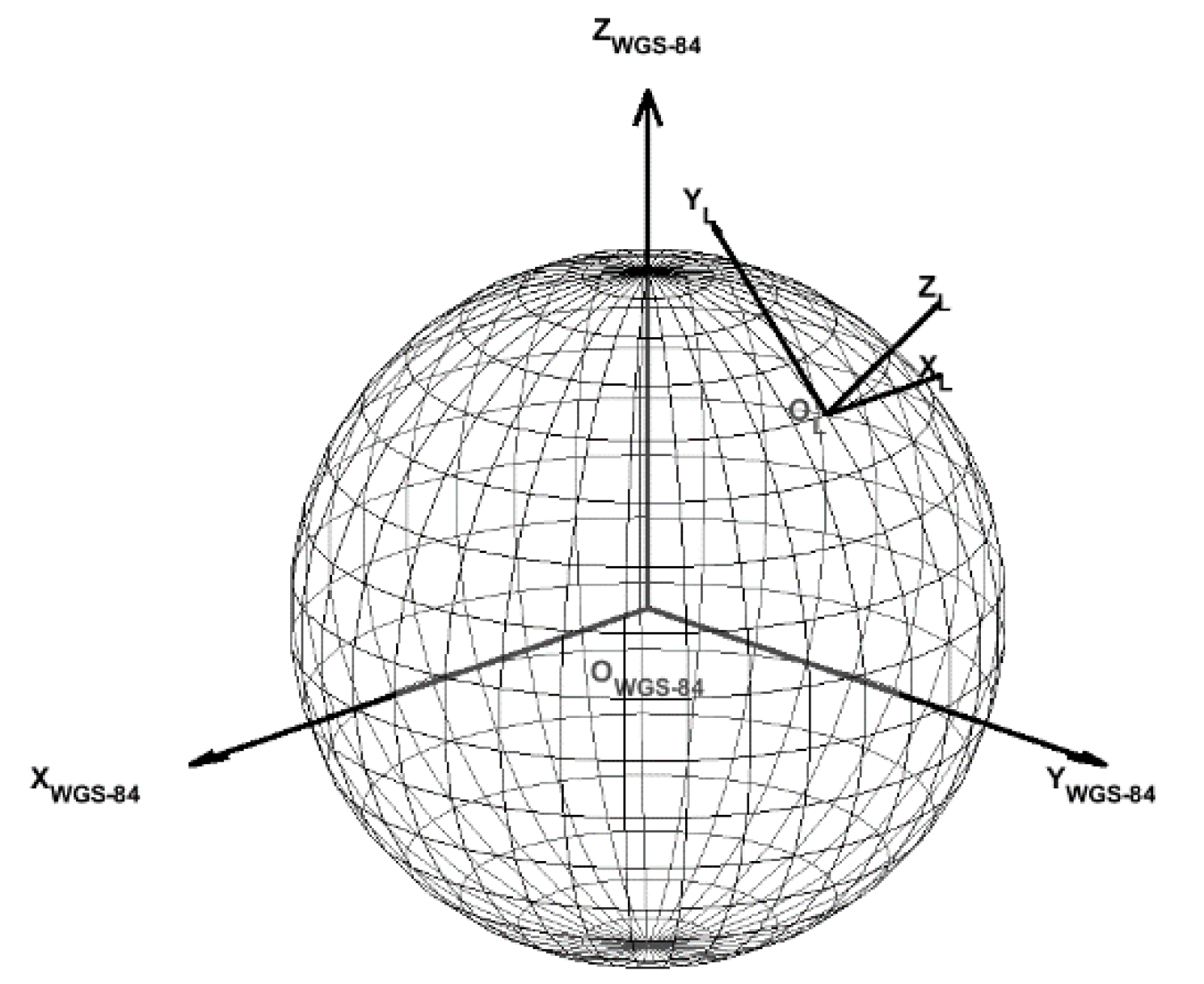
2.2.1. Establishment of the Orchard’s Local Coordinate System and Fruit Tree Distribution Map
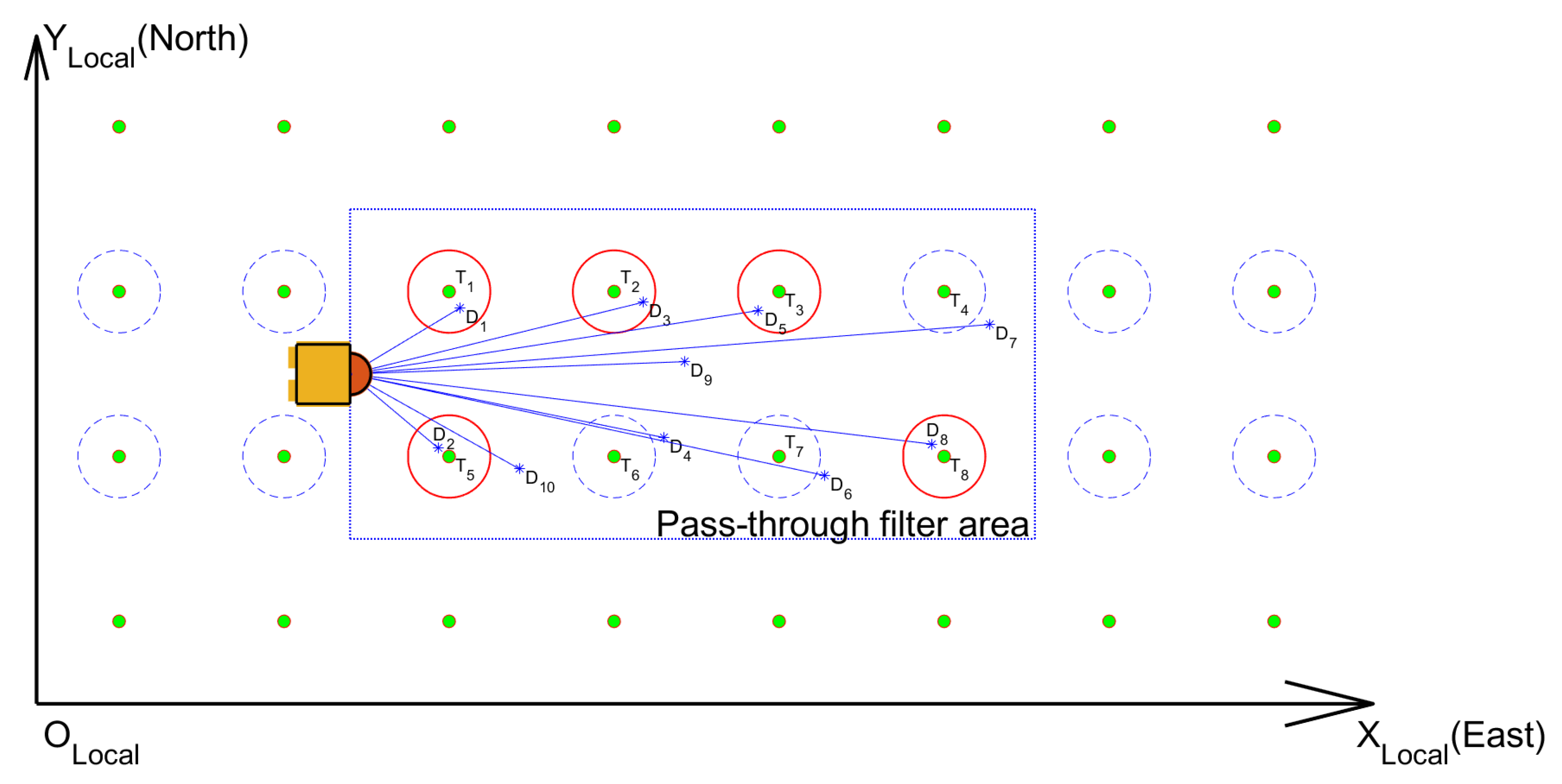
2.2.2. Identification of Fruit Tree Trunks and Acquisition of Trunk Cluster Center Coordinates
2.2.3. Coordinate Transformation of Trunk Cluster Centers into the Orchard’s Local Coordinate System
2.2.4. Matching the Trunk Cluster Centers with the Fruit Tree Distribution Map
2.2.5. Obtaining a Posterior Estimate
2.2.6. Motion Control
2.3. Test Design
2.3.1. Orchard Tests
System Localization Accuracy Tests
2.3.2. Data Processing
3. Test Results and Analysis
3.1. System Localization Accuracy Tests
3.2. Orchard Navigation Tests
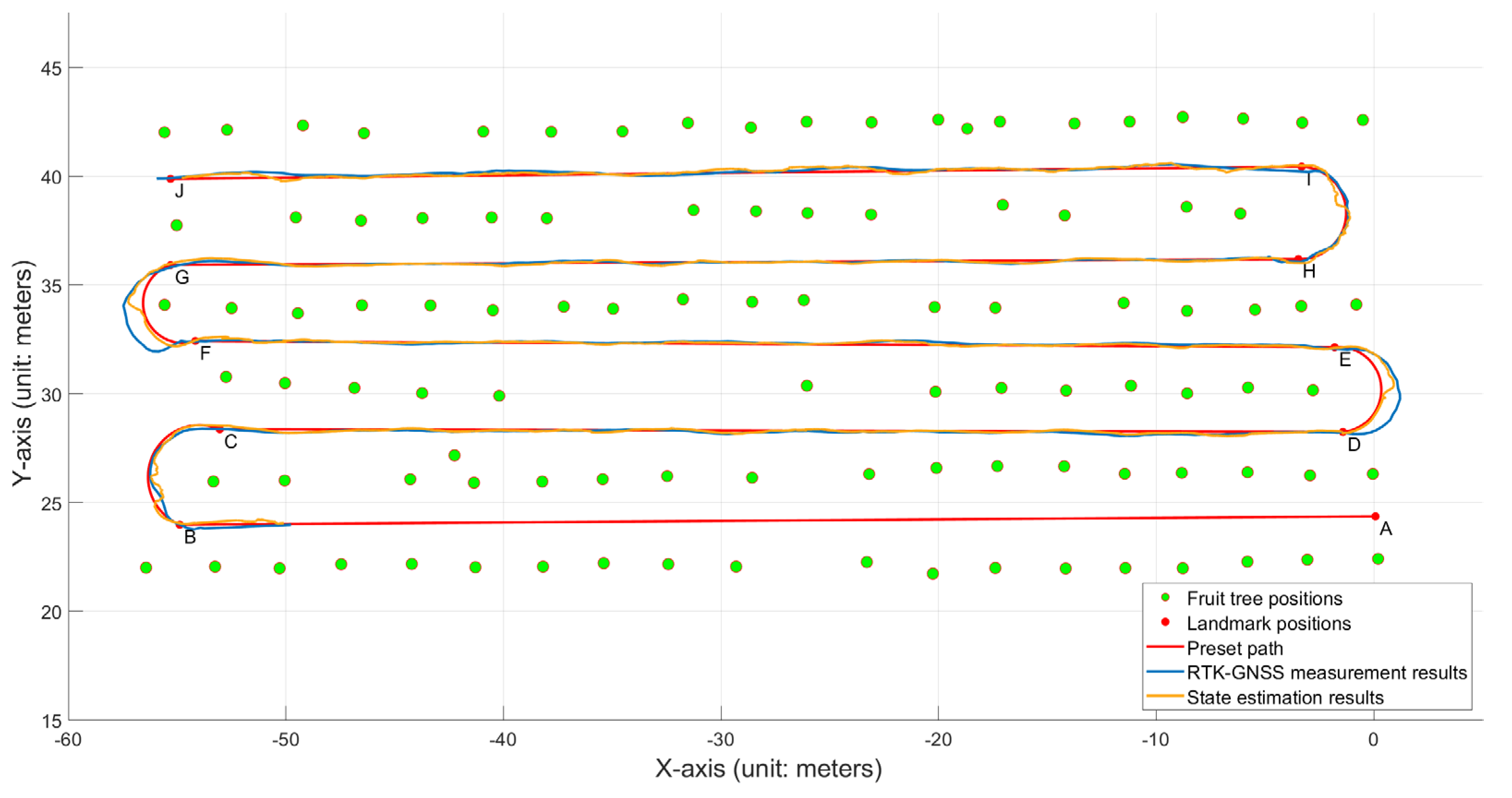
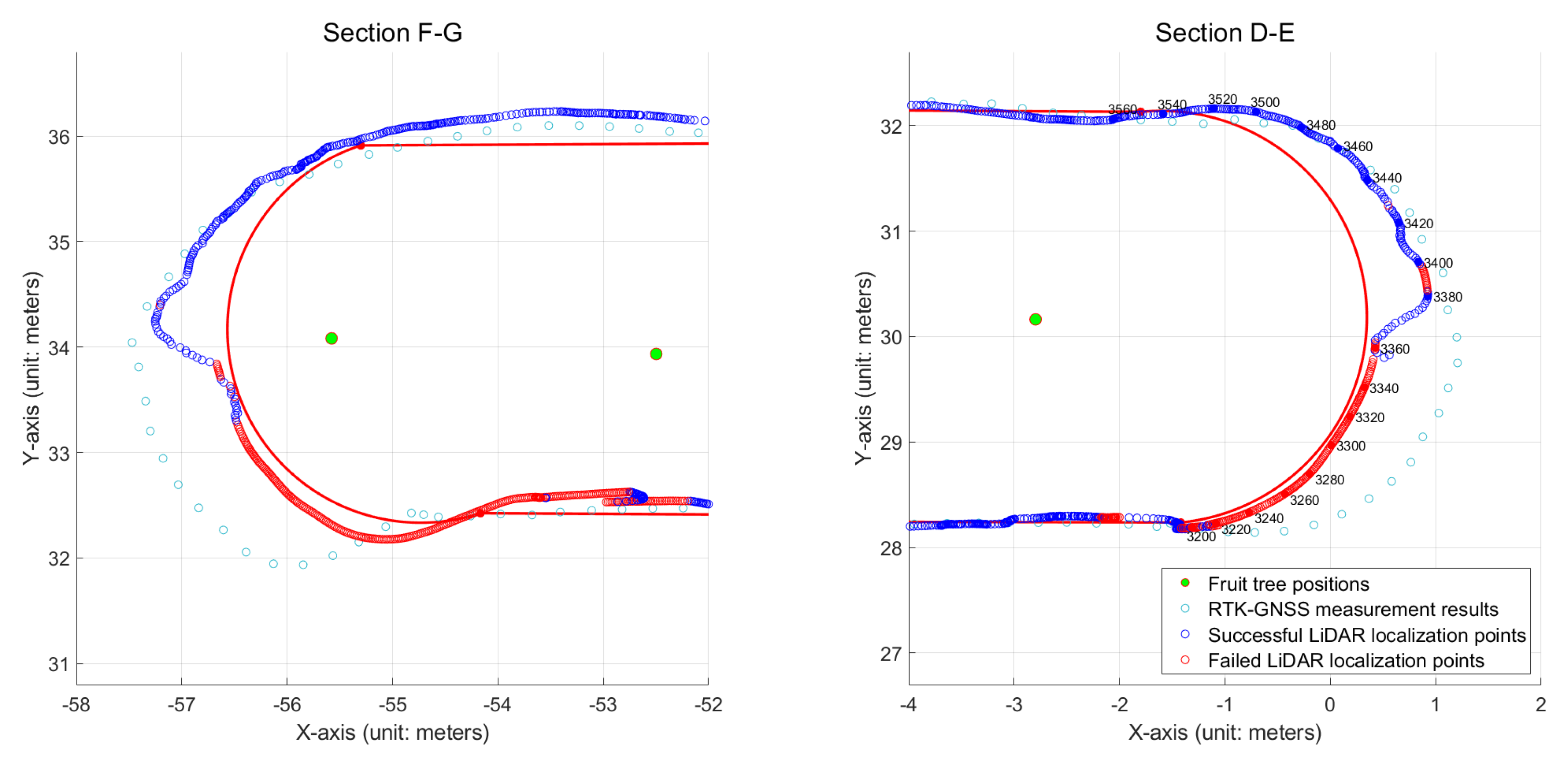
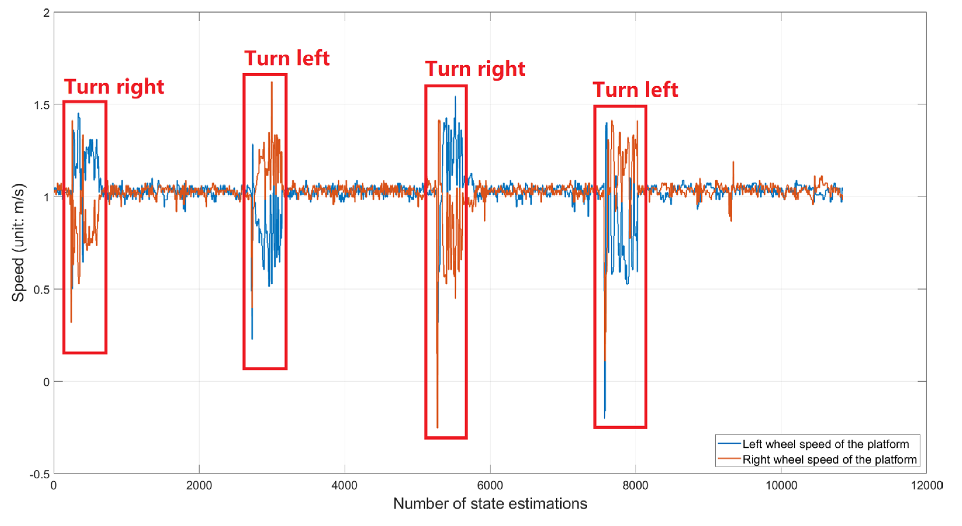
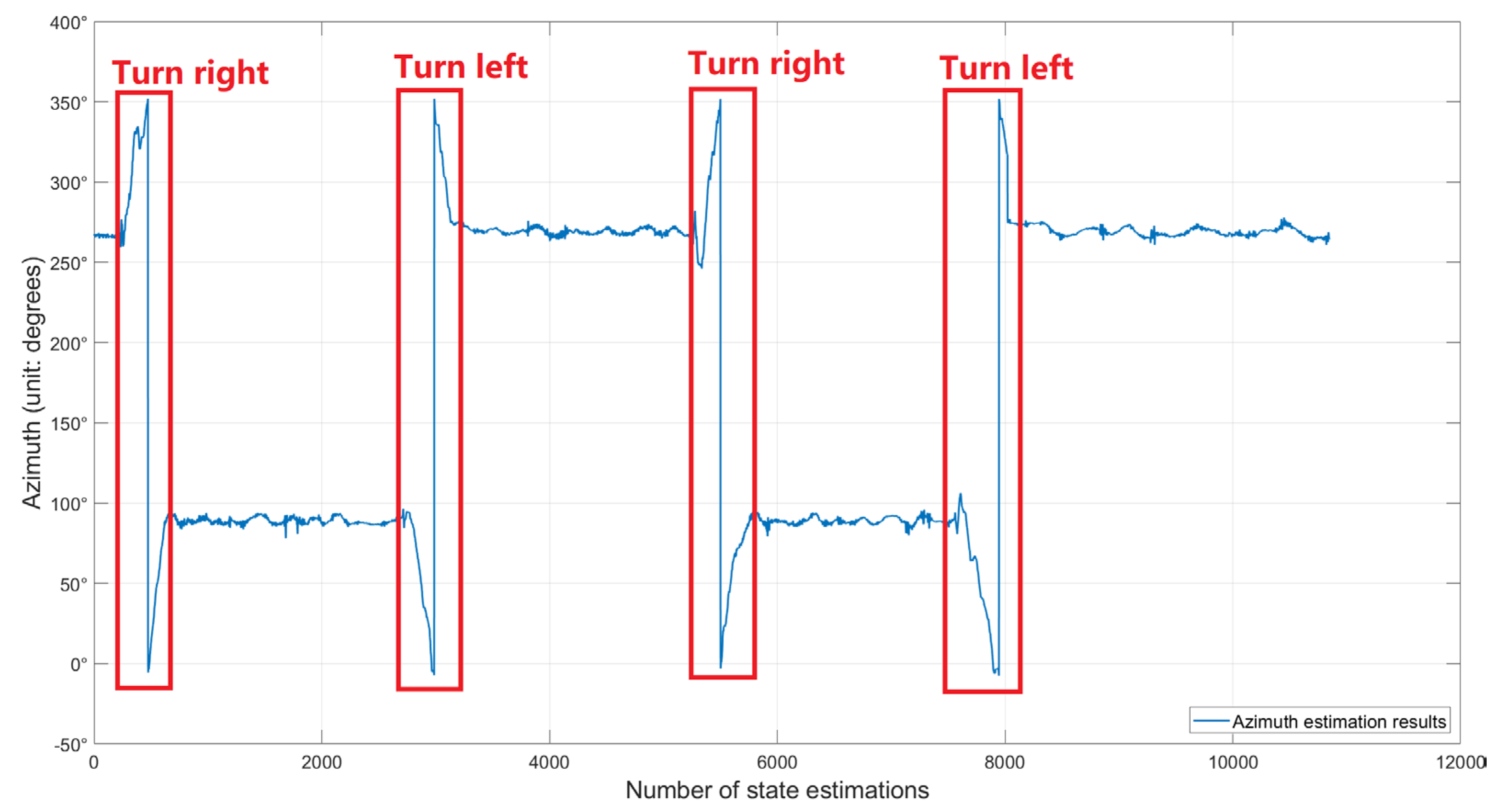
3.2.1. Overall System Navigation Performance Evaluation
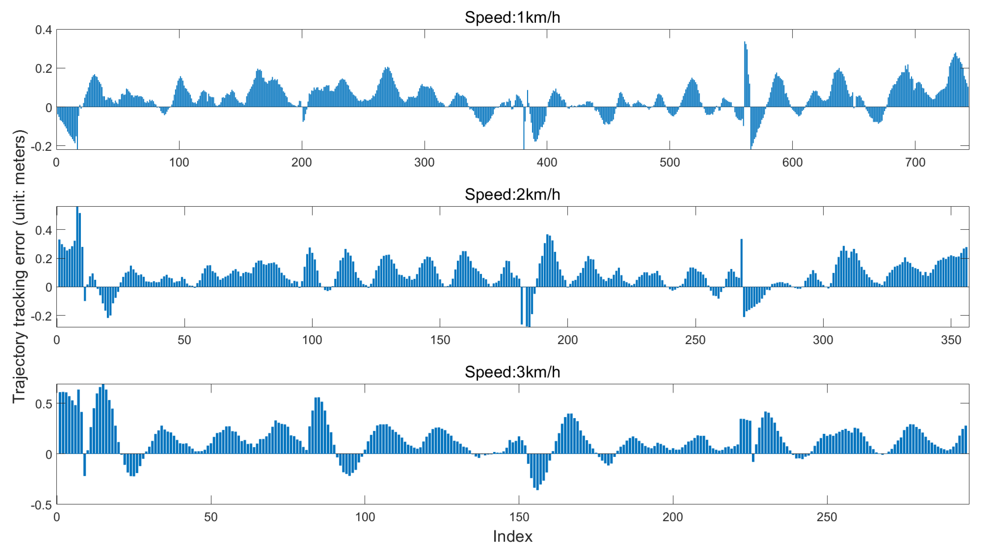
3.2.2. Trajectory Tracking Tests at Different Straight-Line Driving Speeds
3.3. Discussion
3.3.1. Discussion of System Localization Results
3.3.2. Discussion of System Navigation Performance
4. Conclusions
Author Contributions
Funding
Data Availability Statement
Conflicts of Interest
References
- Dou, H.; Chen, Z.; Zhai, C.; Zou, W.; Song, J.; Feng, F.; Zhang, Y.L.; Wang, X. Research progress on autonomous navigation technology for orchard intelligent equipment. Trans. Chin. Soc. Agric. Mach. 2024, 55, 1–22. [Google Scholar]
- Zhang, C.; Yong, L.; Chen, Y.; Zhang, S.; Ge, L.; Wang, S.; Li, W. A rubber-tapping robot forest navigation and information collection system based on 2D LiDAR and a gyroscope. Sensors 2019, 19, 2136. [Google Scholar] [CrossRef] [PubMed]
- Zhang, S.; Guo, C.; Gao, Z.; Sugirbay, A.; Chen, J.; Chen, Y. Research on 2D laser automatic navigation control for standardized orchard. Appl. Sci. 2020, 10, 2763. [Google Scholar] [CrossRef]
- Jiang, S.; Qi, P.; Han, L.; Liu, L.; Li, Y.; Huang, Z.; Liu, Y.; He, X. Navigation system for orchard spraying robot based on 3D LiDAR SLAM with NDT_ICP point cloud registration. Comput. Electron. Agric. 2024, 220, 108870. [Google Scholar] [CrossRef]
- Gu, B.; Liu, Q.; Tian, G.; Wang, H.; Li, H.; Xie, S. Recognizing and locating the trunk of a fruit tree using improved YOLOv3. Trans. Chin. Soc. Agric. Eng. 2022, 38, 122–129. [Google Scholar]
- Han, J.H.; Park, C.H.; Kwon, J.H.; Lee, J.; Kim, T.S.; Jang, Y.Y. Performance evaluation of autonomous driving control algorithm for a crawler-type agricultural vehicle based on low-cost multi-sensor fusion positioning. Appl. Sci. 2020, 10, 4667. [Google Scholar] [CrossRef]
- Han, J.H.; Park, C.H.; Jang, Y.Y.; Gu, J.D.; Kim, C.Y. Performance evaluation of an autonomously driven agricultural vehicle in an orchard environment. Sensors 2021, 22, 114. [Google Scholar] [CrossRef]
- Han, J.H.; Park, C.H.; Jang, Y.Y. Development of a moving baseline RTK/motion sensor-integrated positioning-based autonomous driving algorithm for a speed sprayer. Sensors 2022, 22, 9881. [Google Scholar] [CrossRef]
- Blok, P.M.; van Boheemen, K.; van Evert, F.K.; IJsselmuiden, J.; Kim, G.H. Robot navigation in orchards with localization based on Particle filter and Kalman filter. Comput. Electron. Agric. 2019, 157, 261–269. [Google Scholar] [CrossRef]
- Higuti, V.A.; Velasquez, A.E.; Magalhaes, D.V.; Becker, M.; Chowdhary, G. Under canopy light detection and ranging-based autonomous navigation. J. Field Robot. 2019, 36, 547–567. [Google Scholar] [CrossRef]
- Malavazi, F.B.P.; Guyonneau, R.; Fasquel, J.B.; Lagrange, S.; Mercier, F. LiDAR-only based navigation algorithm for an autonomous agricultural robot. Comput. Electron. Agric. 2018, 154, 71–79. [Google Scholar] [CrossRef]
- Jiang, A.; Ahamed, T. Navigation of an autonomous spraying robot for orchard operations using LiDAR for tree trunk detection. Sensors 2023, 23, 4808. [Google Scholar] [CrossRef] [PubMed]
- Andersen, J.C.; Ravn, O.; Andersen, N.A. Autonomous rule-based robot navigation in orchards. IFAC Proc. Vol. 2010, 43, 43–48. [Google Scholar] [CrossRef]
- Bergerman, M.; Maeta, S.M.; Zhang, J.; Freitas, G.M.; Hamner, B.; Singh, S.; Kantor, G. Robot farmers: Autonomous orchard vehicles help tree fruit production. IEEE Robot. Automat. Mag. 2015, 22, 54–63. [Google Scholar] [CrossRef]
- Libby, J.; Kantor, G. Deployment of a point and line feature localization system for an outdoor agriculture vehicle. In Proceedings of the 2011 IEEE International Conference on Robotics and Automation, Shanghai, China, 9–13 May 2011; IEEE Publications: Piscataway Township, NJ, USA, 2011; pp. 1565–1570. [Google Scholar]
- Hough, P.V. Method and Means for Recognizing Complex Patterns. U.S. Patent No. 3,069,654, 18 December 1962. [Google Scholar]
- Chen, J.; Qiang, H.; Wu, J.; Xu, G.; Wang, Z. Navigation path extraction for greenhouse cucumber-picking robots using the prediction-point Hough transform. Comput. Electron. Agric. 2021, 180, 105911. [Google Scholar] [CrossRef]
- Barawid, O.C., Jr.; Mizushima, A.; Ishii, K.; Noguchi, N. Development of an autonomous navigation system using a two-dimensional laser scanner in an orchard application. Biosyst. Eng. 2007, 96, 139–149. [Google Scholar] [CrossRef]
- Zhou, M.; Xia, J.; Yang, F.; Zheng, K.; Hu, M.; Li, D.; Zhang, S. Design and experiment of visual navigated UGV for orchard based on Hough matrix and RANSAC. Int. J. Agric. Biol. Eng. 2021, 14, 176–184. [Google Scholar] [CrossRef]
- Fischler, M.A.; Bolles, R.C. Random sample consensus: A paradigm for model fitting with applications to image analysis and automated cartography. Commun. ACM 1981, 24, 381–395. [Google Scholar] [CrossRef]
- Guyonneau, R.; Mercier, F.; Oliveira Freitas, G.F. LiDAR-only crop navigation for symmetrical robot. Sensors 2022, 22, 8918. [Google Scholar] [CrossRef]
- Isack, H.; Boykov, Y. Energy-based geometric multi-model fitting. Int. J. Comput. Vis. 2012, 97, 123–147. [Google Scholar] [CrossRef]
- Wang, Y.; Geng, C.; Zhu, G.; Shen, R.; Gu, H.; Liu, W. Information perception method for fruit trees based on 2D LiDAR sensor. Agriculture 2022, 12, 914. [Google Scholar] [CrossRef]
- Shang, Y.; Wang, H.; Qin, W.; Wang, Q.; Liu, H.; Yin, Y.; Song, Z.; Meng, Z. Design and test of obstacle detection and harvester pre-collision system based on 2D lidar. Agronomy 2023, 13, 388. [Google Scholar] [CrossRef]
- Velasquez, A.E.B.; Higuti, V.A.H.; Guerrero, H.B.; Gasparino, M.V.; Magalhães, D.V.; Aroca, R.V.; Becker, M. Reactive navigation system based on H∞ control system and LiDAR readings on corn crops. Precis. Agric. 2020, 21, 349–368. [Google Scholar] [CrossRef]
- Mújica-Vargas, D.; Vela-Rincón, V.; Luna-Álvarez, A.; Rendón-Castro, A.; Matuz-Cruz, M.; Rubio, J. Navigation of a differential wheeled robot based on a type-2 fuzzy inference tree. Machines 2022, 10, 660. [Google Scholar] [CrossRef]
- Hiremath, S.A.; Van Der Heijden, G.W.A.M.; Van Evert, F.K.; Stein, A.; Ter Braak, C.J.F. Laser range finder model for autonomous navigation of a robot in a maize field using a particle filter. Comput. Electron. Agric. 2014, 100, 41–50. [Google Scholar] [CrossRef]
- Thrun, S.; Burgard, W.; Fox, D. Probabilistic Robotics; China Machine Press: Beijing, China, 2017. [Google Scholar]
- Shalal, N.; Low, T.; McCarthy, C.; Hancock, N. Orchard mapping and mobile robot localisation using on-board camera and laser scanner data fusion—Part B: Mapping and localisation. Comput. Electron. Agric. 2015, 119, 267–278. [Google Scholar] [CrossRef]
- Available online: http://www.dfwee.com/h-pd-127.html (accessed on 14 November 2024).
- Available online: https://www.sick.com/cn/zh/catalog/products/lidar-and-radar-sensors/lidar-sensors/lms1xx/c/g91901?tab=downloads (accessed on 14 November 2024).
- Simon, D. Optimal State Estimation: Kalman, H Infinity, and Nonlinear Approaches; John Wiley & Sons, Inc.: Hoboken, NJ, USA, 2006. [Google Scholar]


| State Estimation Point | Number of Trunk Clusters | Number of Successfully Matched Trunk Clusters | Number of Successfully Matched Fruit Trees | Number of Valid Measurements | Localization State |
|---|---|---|---|---|---|
| 3200 | 13 | 1 | 1 | 0 | Failed |
| 3280 | 12 | 1 | 1 | 0 | Failed |
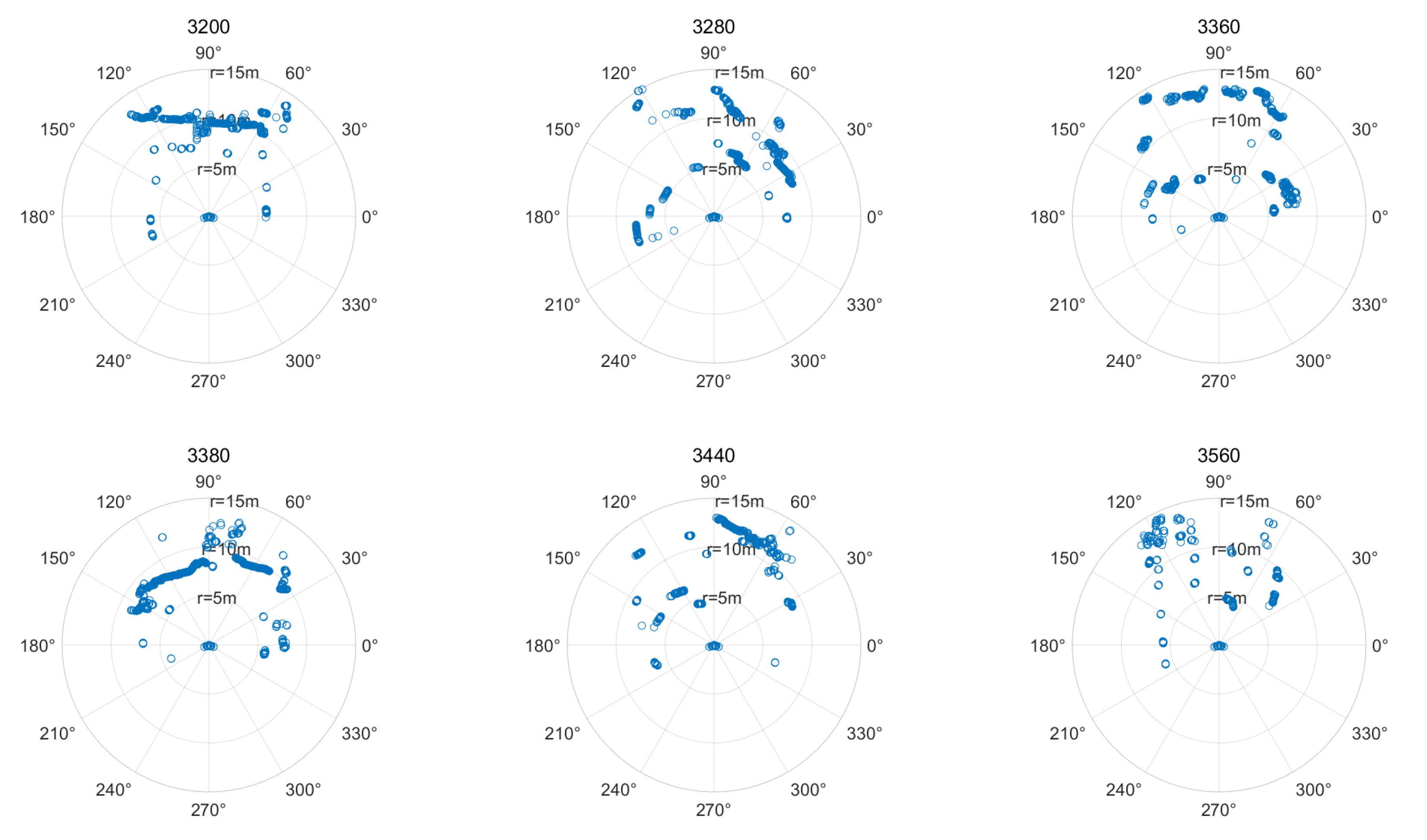
| 3360 | 10 | 3 | 3 | 0 | Failed |
| 3380 | 16 | 5 | 5 | 3 | Success |
| 3440 | 9 | 8 | 8 | 25 | Success |
| 3560 | 13 | 7 | 7 | 21 | Success |
| Speed | Mean Absolute Error of Trajectory Tracking | Standard Deviation of Absolute Trajectory Tracking Error | Maximum Absolute Trajectory Tracking Error | RMS | Proportion of Absolute Error ≥5% |
|---|---|---|---|---|---|
| 1 km/h | 0.07 m | 0.06 m | 0.32 m | 0.09 m | ≥0.18 m (5.79%) |
| 2 km/h | 0.11 m | 0.09 m | 0.56 m | 0.14 m | ≥0.27 m (5.06%) |
| 3 km/h | 0.18 m | 0.14 m | 0.64 m | 0.22 m | ≥0.47 m (5.08%) |
Disclaimer/Publisher’s Note: The statements, opinions and data contained in all publications are solely those of the individual author(s) and contributor(s) and not of MDPI and/or the editor(s). MDPI and/or the editor(s) disclaim responsibility for any injury to people or property resulting from any ideas, methods, instructions or products referred to in the content. |
© 2024 by the authors. Licensee MDPI, Basel, Switzerland. This article is an open access article distributed under the terms and conditions of the Creative Commons Attribution (CC BY) license (https://creativecommons.org/licenses/by/4.0/).
Share and Cite
Su, Z.; Zou, W.; Zhai, C.; Tan, H.; Yang, S.; Qin, X. Design of an Autonomous Orchard Navigation System Based on Multi-Sensor Fusion. Agronomy 2024, 14, 2825. https://doi.org/10.3390/agronomy14122825
Su Z, Zou W, Zhai C, Tan H, Yang S, Qin X. Design of an Autonomous Orchard Navigation System Based on Multi-Sensor Fusion. Agronomy. 2024; 14(12):2825. https://doi.org/10.3390/agronomy14122825
Chicago/Turabian StyleSu, Zhengquan, Wei Zou, Changyuan Zhai, Haoran Tan, Shuo Yang, and Xiangyang Qin. 2024. "Design of an Autonomous Orchard Navigation System Based on Multi-Sensor Fusion" Agronomy 14, no. 12: 2825. https://doi.org/10.3390/agronomy14122825
APA StyleSu, Z., Zou, W., Zhai, C., Tan, H., Yang, S., & Qin, X. (2024). Design of an Autonomous Orchard Navigation System Based on Multi-Sensor Fusion. Agronomy, 14(12), 2825. https://doi.org/10.3390/agronomy14122825