Article

Improving Simulations of Rice Growth and Nitrogen Dynamics by Assimilating Multivariable Observations into ORYZA2000 Model

1
State Key Laboratory of Water Resources Engineering and Management, Wuhan University, Wuhan 430072, China
2
Urban Operation Management Center of Hengsha Township, Shanghai 201914, China
*
Author to whom correspondence should be addressed.
Agronomy 2024, 14(10), 2402; https://doi.org/10.3390/agronomy14102402
Submission received: 4 September 2024 / Revised: 6 October 2024 / Accepted: 14 October 2024 / Published: 17 October 2024

Abstract

:
The prediction of crop growth and nitrogen status is essential for agricultural development and food security under climate change scenarios. Crop models are powerful tools for simulating crop growth and their responses to environmental variables, but accurately capturing the dynamic changes in crop nitrogen remains a considerable challenge. Data assimilation can reduce uncertainties in crop models by integrating observations with model simulations. However, current data assimilation research is primarily focused on a limited number of observational variables, and insufficiently utilizes nitrogen observations. To address these challenges, this study developed a new multivariable data assimilation system, ORYZA-EnKF, that is capable of simultaneously integrating multivariable observations (including development stage, DVS; leaf area index, LAI; total aboveground dry matter, WAGT; and leaf nitrogen concentration, LNC). Then, the system was tested through three consecutive years of field experiments from 2021 to 2023. The results revealed that the ORYZA-EnKF model significantly improved the simulations of crop growth compared to the ORYZA2000 model. The relative root mean squared error (RRMSE) for LAI simulations decreased from 23–101% to 16–47% in the three-year experiment. Moreover, the incorporation of LNC observations enabled more accurate predictions of rice nitrogen dynamics, with RRMSE for LNC simulations reduced from 16–31% to 14–26%. And, the RRMSE decreased from 32–50% to 30–41% in the simulations of LNC under low-nitrogen conditions. The multivariable data assimilation system demonstrated its effectiveness in improving crop growth simulations and nitrogen status predictions, providing valuable insights for precision agriculture.

1. Introduction

Rice is one of the most important cereal crops and serves as a staple food for nearly half of the global population [1,2]. Rice yield is closely linked to nitrogen fertilizer supply, as nitrogen is an essential nutrient for crop growth and development [3]. Accurately assessing crop nitrogen status is crucial for guiding farmland management and ensuring food security [4,5]. Crop models are powerful tools that can effectively characterize crop growth and the responses to nitrogen fertilizer applications [6]. In the past few decades, crop models have been widely used in crop growth and development simulation, water and fertilizer management, and yield forecasting [7,8].
Despite the continuous improvements of crop models, there are still plenty of uncertainties, which may cause discrepancies between simulation results and observed data [9,10]. Specifically, the nitrogen dynamics are often based on the maximum, minimum, and critical nitrogen contents of plants or their organs in most crop models, which should be parameterized for different growth stages [11]. These parameterization techniques cannot adequately capture the dynamics of crop morphology and physiology, limiting the ability to simulate crop nitrogen processes [12]. It was found that the simulation accuracies of crop nitrogen variables were lower than that of the leaf area index (LAI), biomass, and yield by the ORYZA2000 model, which indicated certain structural errors in the nitrogen dynamics [13]. Furthermore, the results in [14] showed that the model performance was poorer under low-nitrogen scenarios, as accurately simulating soil nitrogen mineralization processes became increasingly crucial in these cases, which posed additional challenges. For example, the LAI was found to be overestimated [15] and leaf nitrogen content was underestimated under low-nitrogen scenarios [16] in the applications of the ORYZA2000 model.
The data assimilation (DA) technique incorporates observations into the models and integrates various uncertainties from measured data and model simulations to improve model performance [17,18,19]. Generally speaking, there are three data assimilation techniques, namely, forcing, calibration, and updating strategy [19,20,21]. Compared to the first two methods, the updating method has garnered increasing attention, especially the widely used Ensemble Kalman Filter (EnKF) technique [22,23,24,25]. The EnKF technique is a sequential assimilation method that enables the computation of nonlinear observation operators with low computational requirements while supporting near real-time model simulations [21].
In past studies of crop model data assimilation, observation variables were usually the apparent traits of crop growth and development, such as the LAI, phenology, canopy coverage, and biomass, as well as their growing environments, such as soil water content [20,21]. Among these variables, the LAI was the most frequently used variable because it can effectively capture the comprehensive impact of management and environmental factors on crop growth [25,26]. Moreover, since phenology significantly affects important processes in crop growth and development, it is essential for crop simulation and decision-making [27]. Due to the direct correlation between biomass and yield, biomass was also selected as an observational variable for data assimilation [28]. Most previous studies have acquired only one or two observation variables, and there were few studies on the assimilation of multiple variables simultaneously [20,29]. The value of plant height, the LAI, and soil moisture was explored in sugarcane growth simulations [30]. And, the results in [31] showed that assimilating canopy coverage, biomass, and phenology provided the best performance in the estimation of rice yield.
However, there are still large uncertainties in crop nitrogen simulations, and the assimilation of nitrogen-related variables remains insufficiently explored in existing research [20,21]. Liang et al. [32] pointed out that the crop nitrogen stress factor was a crucial element affecting crop nitrogen absorption and growth simulation, and this factor varied under different crop nitrogen dilution curve methods. Given the importance of nitrogen status for accurately simulating crop growth, it is essential to integrate nitrogen-related observations into the crop model data assimilation framework [33]. With advancements in observation techniques, collecting and interpreting data on various crop states has become much easier [34,35,36]. Despite inherent uncertainties in these observations, integrating multivariate data provides a valuable opportunity to deepen our understanding of crop growth and nitrogen dynamics [30,37]. Crop state variables such as phenology, the LAI, biomass, and leaf nitrogen concentration (LNC) contain abundant information about crop growth and nutrient supply, while the potential of data fusion in the simulations of rice growth and nitrogen dynamics has not been fully investigated.
Therefore, we developed a new multivariable data assimilation system named ORYZA-EnKF by combining the rice growth model ORYZA2000 and the EnKF method. The novelty of this study lies in building a data assimilation system that is capable of integrating multiple variables to address the challenges of inaccurate simulations in rice growth and nitrogen dynamics. Our contribution in this paper is two-fold: (1) the ORYZA-EnKF model assimilates four types of observational variables simultaneously, including the crop development stage (DVS), LAI, total aboveground dry matter (WAGT), and LNC; and (2) mitigates structural errors in nitrogen dynamics of the ORYZA2000 model by assimilating LNC observations, especially when the nitrogen fertilizer is in short supply. Based on a three-year field experiment, this study seeks to (1) conduct a sensitivity analysis to identify the sensitive parameters of the ORYZA2000 model and calibrate the model, (2) evaluate the contributions of various observational variables in the data assimilation system, especially the nitrogen observations, and (3) improve the accuracy of rice growth, nitrogen status simulation, and yield estimation through data assimilation.

2. Materials and Methods

Figure 1 presents a flowchart illustrating the processes of assimilating four types of observational data into the ORYZA2000 crop model simulations by using the EnKF data assimilation algorithm. First, the model is executed using weather data, crop parameters, and soil parameters, followed by a sensitivity analysis to identify the most influential parameters. Field observation data are then assimilated with the model simulations to build the ORYZA-EnKF data assimilation system. The ORYZA-EnKF system is tested using the observing simulation system and the three-year experiment, which were utilized to evaluate the performance of three models: (1) the open-loop model without data assimilation, (2) the ORYZA-EnKF model that assimilates the other three observations but excludes the LNC, and (3) the ORYZA-EnKF model that assimilates all observations, including the LNC. The following section provides a detailed description of the data and methods used in this study.

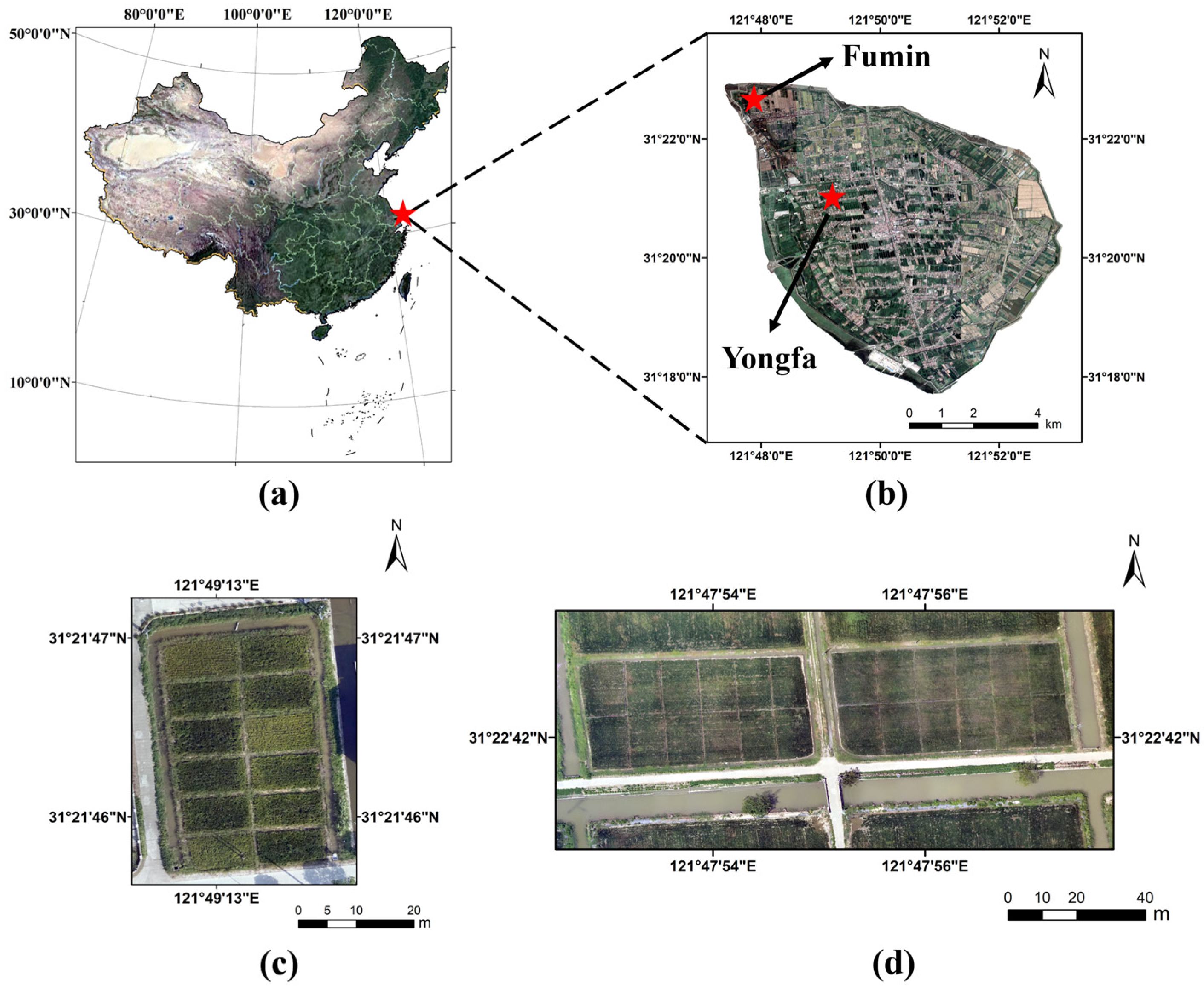
2.1. Description of the Experimental Area

The experimental site is located in Hengsha township, Chongming district, Shanghai city, China (31.34° N, 121.84° E). The climate is subtropical monsoon, with an average annual temperature of 15.4 °C, and an average annual rainfall of 1100 mm. The soil type at the experimental site is sandy loam, with the top 20 cm layer containing 1.80–2.27 g kg−1 of total nitrogen (TN), 6.32–9.53 mg kg−1 of nitrate nitrogen (NO3-N), and 3.45–5.09 mg kg−1 of ammonium nitrogen (NH4+-N). The rice varieties grown in the experimental area are primarily japonica varieties. The planting season is from June to November. The experiments in 2021 and 2022 were conducted in Yongfa village, and the 2023 experiment was carried out in Fumin village. The layouts of the experimental plots are shown in Figure 2.

2.2. Field Data Collection

During the three-year experiment, Nanjing 46 (NJ46) was planted in 2021 and 2022, and Chongxiangjing 201 (CXJ201) was used in 2023. Each plot was approximately 60.5 m2 (11 m × 5.5 m) in 2021 and 2022, and the area was approximately 150 m2 (15 m × 10 m) in 2023. Details of these experiments are presented in Table 1. The three trials were named 2021-YF, 2022-YF, and 2023-FM based on the year and field location. A variety of nitrogen treatment levels were established in the three-year experiment, with each application level replicated three times. The nitrogen application rates in the 2021 and 2022 experiments were determined based on local agricultural management practices, and the different treatments were designed to investigate the effects of varying nitrogen levels on rice growth. In the 2023 experiment, nitrogen application rates were determined based on the crop growth conditions and previous experimental research. Due to the use of drones for fertilization in 2023, accurately applying nitrogen to small plots was quite challenging, which led to the absence of a zero-nitrogen group. As a result, we eliminated the zero-nitrogen treatment in 2023 and replaced it with a low nitrogen application level (N58).
Weather stations were installed to collect long-term weather data, including solar radiation, minimum and maximum temperatures, relative humidity, wind speed, and rainfall. DVS was monitored by randomly selecting 3–5 rice plants in the field and closely observing the morphology of stems, leaves, ears, and flowers. Then, the rice phenology was recorded numerically according to the code of Lancashire et al. [38]. The LAI represents the leaf area index [39] and was measured using the LAI-2200C Plant Canopy Analyzer (LI-COR, Lincoln, NE, USA). To avoid the influence of direct sunlight on the measurements, the observations were acquired on a cloudy day with uniform cloud cover or at sunrise or sunset. WAGT was obtained using destructive sampling and three bundles of rice plants were randomly selected from each field. The aboveground parts of the rice plants were dried at 70 °C to a constant weight, and then the WAGT of the plot scale was calculated through multiplying the dry weight of a single bundle by the plant density.
After the WAGT measurement, leaves were manually separated from rice plants, and then were ground, sifted, dried and weighed for chemical analysis in the laboratory. Rice LNC was measured using the Kjeldahl method by a K9840 Kjeldahl Analyzer (Hanon, Dezhou, China) in 2021 and the Dumas method by an EMA 502 CHNS-O element analyzer (VELP, Usmate Velate, Italy) in 2022 and 2023. Both methods are widely used for plant and soil nitrogen measurements, and the data obtained from the two methods are very close, with minimal differences [40,41,42]. When the rice reaches maturity, a sample square of 1 m2 (1 m × 1 m) was selected from each test plot. All above-ground parts of the rice were collected, and the dry weights of the rice yield (water content is uniformly converted to 14%) were measured.
In the continuous three-year experiment, we conducted observations throughout the entire rice growth period. During the vegetative growth stage, the observation frequency was approximately every 10 days, while in the reproductive growth stage, it was about every 20 days. In 2021, we performed 7–9 samplings for various observational variables, 8–9 samplings in 2022, and 7 samplings in 2023. The temporal resolution of data acquisition enabled us to effectively capture the dynamic changes in the crop across different growth stages.

2.3. ORYZA2000 Model

The ORYZA2000 model was employed as the base model for data assimilation due to the fact that it has been widely applied in rice cultivation and management studies [43]. The ORYZA2000 model can quantitatively and dynamically describe the rice growth and development processes under changing climate conditions, as well as water and nitrogen constraints [44,45]. The main processes simulated by the ORYZA2000 model include phenological development, CO2 canopy assimilation, leaf area growth, and dry matter distribution. The nitrogen module of the model encompasses key processes such as the calculation of soil nitrogen availability, the dynamics of crop nitrogen uptake and utilization, and the mechanisms of nitrogen stress response [15].

2.3.1. Crop Growth Module

Under conditions of potential production, the ORYZA2000 model first calculates the instantaneous photosynthetic rate of each leaf, and then integrates the whole canopy according to the canopy green area index.
A m = 49.57 / 34.26 × 1 exp 0.208 CO 2 60 / 49.57
where Am is the maximum CO2 assimilation rate per hour of a single leaf (kg CO2 ha−1 leaf h−1), which is related to the concentration of CO2 in the air.
In the early growth stage, the canopy of rice is not closed, and the growth of green leaf area is not limited by dry matter growth. The growth rate is affected by the accumulated temperature:
G L A I = G L A I t 0 × exp R G R L × t s
where GLAI is the green leaf area index (ha ha−1), GLAIt0 is the initial GLAI (ha ha−1). RGRL is the relative growth rate of leaf area ((°Cd) −1). ts is the accumulated temperature (°Cd).
When GLAI exceeds 1, the development of the green leaf area is determined by both leaf mass and the specific leaf area:
G L A I = W L V G × S L A
where WLVG is the mass of the green leaf (kg ha−1). The SLA is the specific leaf area (m2 kg−1) and varies with the growth period.
The LAI is calculated as follows:
P A I = G L A I + Y L A I + S A I + E A I
Y L A I = W L V D × S L A × L S H R I N K
S A I = W S T × S S G A
E A I = W S O × S G A
where YAI is the yellow leaf area index (ha ha−1), SAI is stem area index (ha ha−1), EAI is the panicle area index (ha ha−1). SSGA and SGA are the area coefficients of stems and ears (m2 kg−1), respectively. LSHRINK is the coefficient of leaf area shrinkage (-).

2.3.2. Nitrogen Dynamics

The simulation of soil nitrogen is simplified by the ORYZA2000 model, which only considers soil-mineralized nitrogen and nitrogen from exogenous fertilizer:
T N S O I L = N F E R T P + S O I L S P
N F E R T P = N f e r × R E C O V
where TNSOIL is the daily nitrogen available from the soil (kg N ha−1 d−1). NFERTP is the nitrogen from applied fertilizers (kg N ha−1). Nfer is the applied fertilizer (kg N ha−1), and RECOV is the crop nitrogen recovery coefficient (-). SOILSP is soil-mineralized nitrogen (kg N ha−1 d−1). When crops need to absorb nitrogen from the soil, the soil-mineralized nitrogen is first used, and fertilizer nitrogen is only consumed if the soil-mineralized nitrogen is not enough to meet the crop nitrogen demand.
The ORYZA2000 model calculates the potential nitrogen demand of plants organs:
N D E M L = W L V × N M A X L A N L V
N D E M S = W S T × 0.5 × N M A X L A N S T
where NDEML and NDEMS are the daily nitrogen requirements of leaf and stem organs (kg N ha−1 d−1). WLV and WST are the leaf and stem masses (kg ha−1). NMAXL is the maximum leaf nitrogen concentration (kg kg−1). The model assumes that the stem has half the nitrogen concentration of the leaf. ANLV and ANST are the accumulated nitrogen content (kg N ha−1) in leaf and stem organs.
The total crop nitrogen requirement NDEMC (kg N ha−1) is calculated as follows:
N D E M C = N D E M L + N T L V + N D E M S + N T S T + N D E M S X N T S O
where NDEMSX is the maximum daily nitrogen requirement of crop storage organs (kg N ha−1 d−1). NTLV, NTST, and NTRT are the amounts of nitrogen actually transferred daily from leaves, stems, and roots to storage organs (kg N ha−1).
NUPP is the daily amount of nitrogen that crops can absorb from the soil (kg N ha−1 d−1):
N U P P = M I N N M A X U P , T N S O I L
where NMAXUP is the maximum amount of nitrogen that a rice plant can absorb per day (kg N ha−1 d−1).
Then, the crop nitrogen content of each organ can be calculated, taking the leaf organ as an example:
A N L V = A N L V + N L V
L N C = A N L V / W L V
where ANLV is the nitrogen accumulation of leaf organs (kg N ha−1), LNC is the leaf nitrogen concentration (kg kg−1).

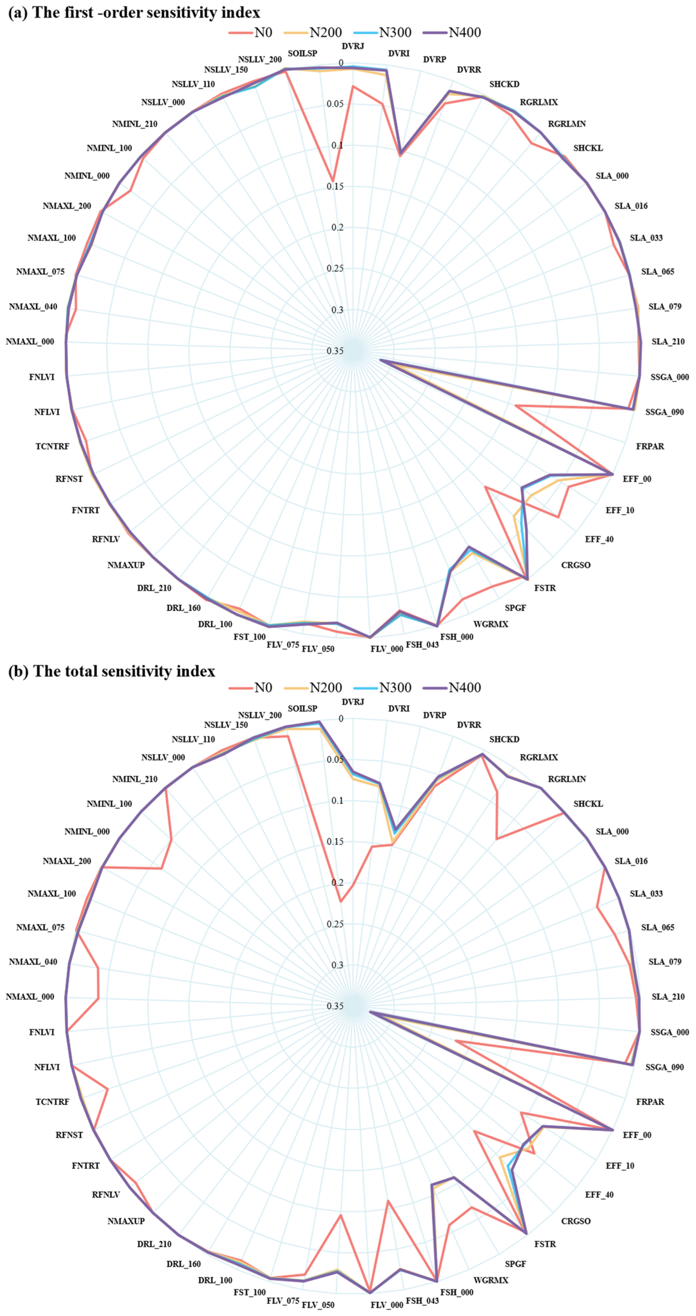
2.4. Parameter Sensitivity Analysis

Crop models typically involve many parameters, and their performances are highly dependent on these parameters [46]. Sensitivity analysis is the common strategy to identify the parameters that significantly influence crop and environmental variables of interest [47,48]. In this study, the Sobol global sensitivity analysis algorithm was employed to quantify the sensitivity indices of key state variables in crop model simulations, thereby identifying the most sensitive parameters [49,50].
The Sobol method is based on variance decomposition, which can deal with nonlinear and non-monotonic functions and models. The model output Y can be expressed as a function of various parameters:
Y = f X 1 , X 2 , , X n
where Y is the model output, X1, X2, …, Xn are a set of parameters; f represents the corresponding relationship between Y and X. According to the formula of variance decomposition, the total variance of the model output can be decomposed into the variance of each parameter and parameter interaction:
V ( Y ) = i = 1 n V i + i = 1 n 1 j = i + 1 n V i j + + V 1 , 2 , , n
where V(Y) is the total variance of model output, Vi is the independent variance of each parameter; Vij is the variance caused by both parameters Xi and Xj. Therefore, the corresponding sensitivity indices can be calculated according to the variance component of each parameter:
S i = V i V Y
S i j = V i j V Y
S T i = 1 V i V Y
where Si refers to the first-order sensitivity index of parameter Xi, which is the influence contribution of a single parameter Xi to the model output. The larger the value of Si, the greater the uncertainty caused by the change in parameter Xi within its uncertainty range to the model results. Sij is a second-order sensitivity index, which represents the influence of the combination of parameters Xi and Xj on the model output. STi is a total order sensitivity index that represents the total contribution of the parameter Xi to the model output, including the influence of the individual Xi parameters as well as the influence of the mixed effects of the parameters.
To investigate the impact of different nitrogen application treatments on the sensitivity analysis results, four nitrogen application scenarios (N0, N200, N300, N400) were set up in the sensitivity analysis simulation based on the nitrogen treatments from the 2021 field trial. Considering the research requirements of this study, four key state variables (LAI, WAGT, LNC, and rice yield) were selected for sensitivity analysis. Based on the existing studies on the ORYZA2000 model, we selected 53 parameters for the sensitivity analysis, including those related to the growth period, leaf area growth, crop photosynthesis, dry matter distribution, and nitrogen processes. For most parameters, the prior values were obtained from the default values in the model files, while some parameter values were based on data from the literature [39,51]. The parameters and their prior values are detailed in Table S1, with uncertainty set at ±30% of the prior value [52].
The sensitivity analysis was performed on a computer equipped with an Intel Core i5-12400F processor (2.50 GHz), 32 GB of DDR4 RAM, and a 1 TB SSD for storage, ensuring sufficient computational power for efficient and accurate simulations. The sensitivity analysis was conducted using Sensitivity Analysis Library (SALib, version 1.4.7) implemented in Python (version 3.9), which is a freely available and open-source package. This package provides a range of methods for assessing the sensitivity of model outputs to changes in input parameters, making it a valuable tool for our analysis.

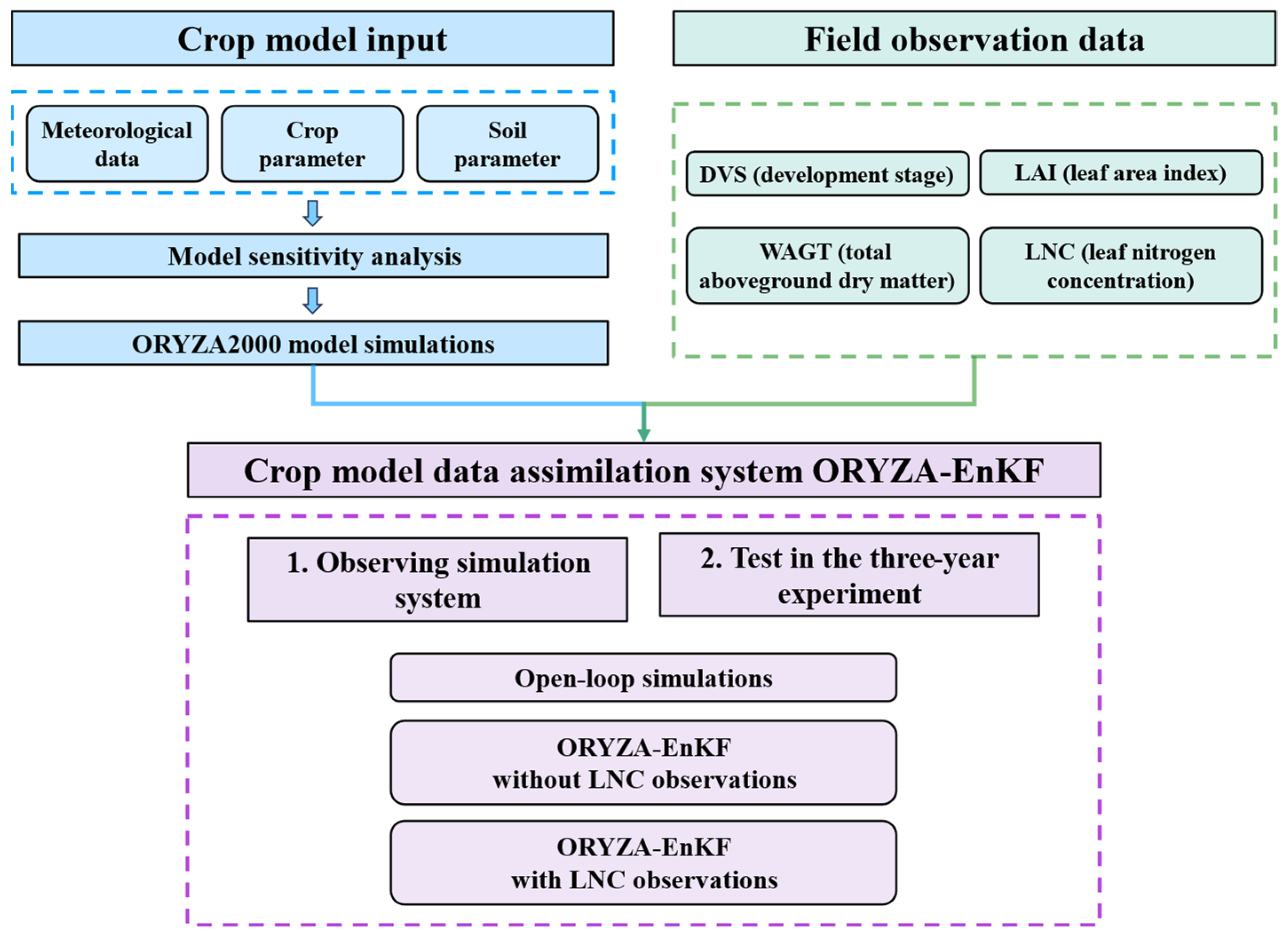
2.5. ORYZA-EnKF Data Assimilation Framework

2.5.1. Ensemble Kalman Filter

The data assimilation method is crucial for the model prediction and computational efficiency. The EnKF algorithm was used in this study to assimilate observed data and update the model. The EnKF can effectively handle high-dimensional nonlinear processes, making it well-suited for crop model data assimilation [25,53]. As a sequential assimilation algorithm, the EnKF simulates the model forward, incorporates new observations, and updates the state matrix using the Kalman filter algorithm. The updated state set then becomes the initial value for the next simulation step, allowing the model to continuously move forward. The iterative process ensures that the model state and parameters are regularly updated with continuous observation data [22].
The EnKF algorithm first constructs a state matrix composed of model parameters, state variables, and observed variables:
y t = m t T , u t T , d t T
where, yt is the state matrix of the model at time t, and its dimension is Ny = Nm + Nu + Nd. mtT is a model parameter matrix, and utT is composed of model state variables. In crop models, it generally refers to physical quantities such as the LAI and WAGT, which are driven by meteorological conditions and vary with time. dtT is a matrix of observations. The observations of the model can be transformed by the observation operator:
d t = H y t
H = 0 , I
where H refers to the observation operator, 0 is an Nd × (Nm + Nu) dimensional matrix in which all elements are 0, I is an identity matrix with dimensions Nd × Nd.
When the model runs to the time t, the calculated state matrix can be updated through the EnKF algorithm:
y t a = y t p + K t d o b s , t H t y t p
where y t a represents the updated state matrix, y t p represents the state matrix when the model runs to t, dobs,t represents the perturbed observation, Kt is the Kalman gain at time t. The Kalman gain can be calculated from the covariance matrix of the sample set:
K t = C y t p H t T H t C y t p H t T + C d o b s , t 1
y t p ¯ = 1 N i = 1 N y t , i p
C y t p = 1 N 1 i = 1 N y t , i p y t p ¯ y t , i p y t p ¯ T
where C y t p refers to the prior covariance matrix of the state vector at time t, C d o b s , t is the observation error. y t p ¯ is the average value of the state matrix at time t, i is the sample sequence number.
Combined with the Monte Carlo method, the EnKF calculates the covariance in the Kalman filter using sample simulations. Many different groups of samples can be constructed by the parameters of the discrete model, and the sample set can be used to reflect the probability characteristics of the state vector. Running the crop model generates a series of simulated values, from which the covariance of these samples can be calculated. This calculation provides the Kalman gain and the updated state matrix of the model.

2.5.2. Observing Simulation System

To better explore the ORYZA-EnKF data assimilation system on crop growth simulation and prediction, this study employed the observing simulation system (OSS) to evaluate the performance of data assimilation [53,54]. The implementation steps of the OSS are as follows: (1) Select a set of default parameters and run the crop model, commonly referred to as an open-loop simulation. (2) Use these default parameters as a baseline, and establish a set of “true” parameter values, under the assumption that this set accurately represents the “real” model behavior. The crop model is then executed with these parameters to generate continuous simulated values for various state variables, which are subsequently treated as the observation data. (3) The observations are assimilated into the open-loop model from the first step, and the assimilated model results are compared with the “true” simulated values. This comparison allows for the evaluation of the performance of the data assimilation system.
Unlike previous data assimilation studies, this research not only utilized commonly used LAI observations but also assimilated other variables. Six cases were designed based on the OSS. Case 1 assimilated all observed variables (DVS, LAI, WAGT, and LNC), and Cases 2–5 assimilated each single observed variable individually. Case 6 represented the scenario where all variables were assimilated except LNC. Observation uncertainty was defined as 10% of the standard deviation of the “true” simulated observations. Observations were taken every 10 days throughout the entire rice growth period. It was generally found that larger sample sizes produced more stable results, but they also required more computational resources and time. When using the EnKF algorithm for crop model data assimilation, the simulation accuracy improvement became minimal once the sample size exceeded 50, and as few as 10 samples were sufficient for assimilation in some years [23,55]. To strike a balance between precision and computational efficiency, this study adopted a sample size of 100 for the discretization of uncertainty parameters.
The crop model data assimilation was conducted in Microsoft Visual Studio and utilized the same computer that was used for the sensitivity analysis. Since the ORYZA2000 model is an open-source model written in Fortran, the ORYZA2000 and ORYZA-EnKF models were implemented using Fortran, enabling efficient data processing and integration.

2.6. Evaluation Method

As widely used standard metrics in past studies, the RMSE (the root mean squared error) and RRMSE (relative root mean squared error) were employed to evaluate the model performance in the simulations of crop growth and nitrogen dynamics, which can be calculated as follows:
R M S E = i = 1 N y i - y ^ i 2 / N
R R M S E = R R M S E / y ¯
where N denotes the number of samples, y i and y ^ i represent the observed state variables and model simulations, y ¯ i is the average value of observations. The RRMSE was employed to avoid the effects of changes in state variables caused by the crop growth stages. Compared to other evaluation metrics, the RMSE and RRMSE could provide a more comprehensive error analysis [24,39]. And, a smaller value of RMSE and RRMSE indicates a higher simulation accuracy of the model.

3. Results and Discussion

3.1. ORYZA2000 Model Parameter Sensitivity Analysis

Figure 3 illustrates the first-order and total sensitivity index of rice yield under four nitrogen application scenarios. As can be seen from Figure 3a, the parameters SOILSP (the nitrogen mineralization rate), FRPAR (the fraction of short-wave radiation that is photosynthetically active), CRGSO (the carbohydrate requirement for storage organ dry matter production), and DVRP (the development rate in panicle development) were sensitive under N0 scenario. When the N rate was 200 kg N ha−1, FRPAR, DVRP, EFF_40 (the initial light-use efficiency at temperature 40 °C) and SPGF (the spikelet growth factor) had significant effects on rice yield, and FRPAR, DVRP, EFF_40, and SPGF were important under the N300 scenario and the N400 scenario. It is obvious that FRPAR and DVRP were highly sensitive under all four nitrogen application scenarios. FRPAR refers to the proportion of photosynthetically active radiation in short-wave radiation, which directly influences the energy available for crop photosynthesis [56]. DVRP is the phenological growth rate of panicle development and plays a key role in the formation of rice panicles [57]. Therefore, the two parameters had a significant impact on rice yield.
SOILSP was the most sensitive parameter when no exogenous nitrogen fertilizer was applied, as rice rely solely on soil-mineralized nitrogen to meet crop nitrogen requirements [58]. When nitrogen nutrients are abundant, yield is more significantly influenced by rice photosynthesis and panicle development. FRPAR and EFF_40 are directly related to photosynthetic efficiency, and changes in DVRP and SPGF affect panicle formation. As a result, these parameters were more sensitive under high-nitrogen scenarios [52,57].
The total sensitivity index in Figure 3b reflects the overall effect of model parameters on rice yield. It can be found that the number of sensitive parameters increased, especially those related to rice phenology (DVRJ, DVRI, DVRP, and DVRR). This is mainly because the growth period influences many other processes in the ORYZA2000 model, such as dry matter distribution, which changes with the crop growth stages [59]. A larger proportion of dry matter is allocated to leaf organs when the rice plants are very small. As the rice grows, an increasing amount of dry matter is distributed to the stem and panicle organs [52].
Figure 3. Sensitivity indices of parameters in the ORYZA2000 model for rice yield under different nitrogen application scenarios: (a) the first-order sensitivity index and (b) the total sensitivity index. N0, N200, N300, and N400 refer to the total N rate of 0, 200, 300, and 400 kg N ha−1, respectively.
Agronomy 14 02402 g003
Figures S1–S4 show the results of the first-order sensitivity index and the total sensitivity index for LNC at different growth stages under four nitrogen application scenarios. It is clear that the sensitive parameters under the N0 scenario were notably different from those under the N400 scenario. SOILSP and the parameters related to the growth period were more important under the N0 scenario. When the nitrogen fertilizer supply was sufficient, SOILSP was no longer important. Under the N400 scenario, the most sensitive parameters were the NMAXL series parameters, which represent the maximum values of rice LNC [51]. For example, NMAXL_040 was pivotal for simulating rice LNC when DVS was 0.40, NMAXL_100 and NMAXL_200 were important parameters at DVS 1.00 and 2.00, respectively. Without nitrogen stress impacting rice growth, LNC reaches its maximum levels, and follows a decreasing dilution pattern [60]. Therefore, the NMAXL series parameters became the most sensitive parameters in this scenario.
The parameter sensitivity analysis results for the LAI under the N0 scenario were shown in Figure S5. DVRJ, RGRLMX (the maximum value of the relative growth rate of leaf area) and SOILSP were important parameters when DVS was 0.40, highlighting the significance of the growth period and soil nitrogen supply at this stage. RGRLMX was sensitive because the LAI mainly depended on green leaves at the early stage, and the green leaf area was experiencing exponential growth, which was directly related to the relative growth rate of leaf area [61]. When DVS was 0.65, DVRJ (the development rate in the juvenile phase), DVRI (the development rate in the photoperiod-sensitive phase), SLA_065 (the specific leaf area at DVS 0.65), FLV_050 (the fraction of shoot dry matter allocated to leaves at DVS 0.50), and SOILSP were crucial parameters, as LAI growth at this stage is influenced by the leaf dry weight and specific leaf area [59]. Figures S6–S8 show the parameter sensitivity analysis results for the LAI under the N200, N300, and N400 scenarios. When the nitrogen fertilizer supply was sufficient, the sensitive parameters were similar to those under the N0 scenario except SOILSP. Important parameters included DVRJ, DVRI, FRPAR, the SLA series, and the FLV series. Figures S9–S12 show the parameter sensitivity analysis results for WAGT under four nitrogen application scenarios. The important parameters for WAGT were almost consistent with those for the LAI. For instance, DVRJ also had a significant impact on WAGT simulation results during the early growth stage. The main difference was that the LAI showed a strong sensitivity to the FLV series parameters and SLA series parameters, whereas WAGT was more influenced by the FSH (the fraction of total dry matter allocated to shoots) series parameters.

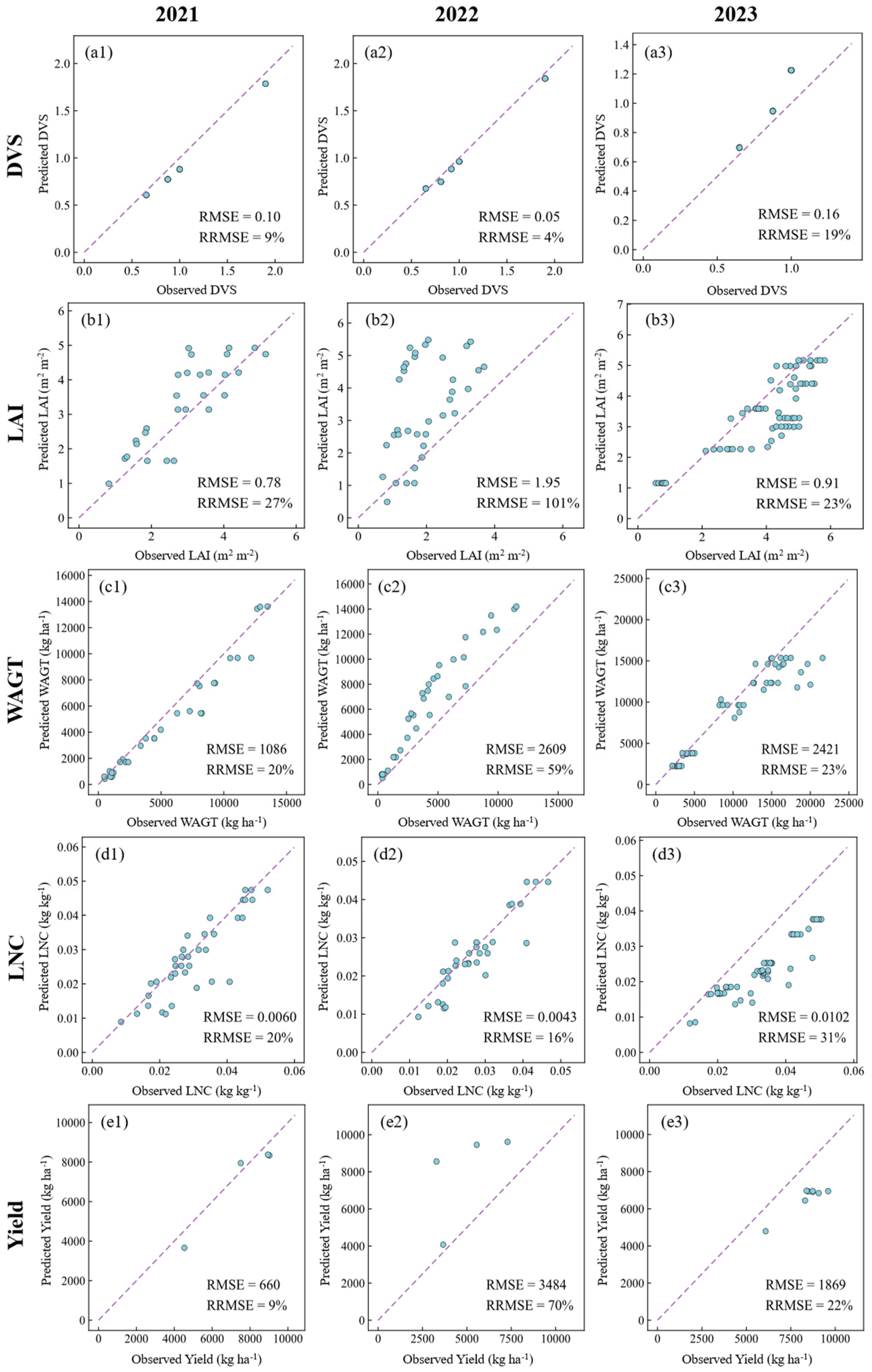
3.2. ORYZA2000 Model Calibration

It was observed that only a few parameters played significant roles in the model simulation results. Therefore, this study employed a trial-and-error approach to adjust these sensitive parameters, aiming to minimize the errors between the simulation results and observations. The observed data in 2021 and 2022 were utilized for parameter calibration, and the data in 2023 were used for validation.
Table 2 shows the evaluation accuracy of five key state variables simulated by the ORYZA2000 model. At the calibration stage, DVS and LNC were simulated with high accuracy, achieving RMSE values of 0.08 and 0.0053, and RRMSE values of 7% and 18%, respectively. However, the simulation accuracy of other variables was low, particularly for the LAI with an RMSE of 1.55 and an RRMSE of 65%. Model simulations for the LAI, WAGT, and yield improved in the validation period, while accuracy declined for DVS and LNC. In general, by fine-tuning sensitive parameters, the ORYZA2000 model can effectively simulate the main state variables in the rice growth and development processes [62,63].
However, it should be recognized that the simulations for the LAI, WAGT, and yield exhibited limited accuracy during the calibration period, which might be attributed to inter-annual differences. Then, the simulation results were divided by year and were illustrated in Figure 4. As depicted in this figure, there was a notable disparity in the calibration results between 2021 and 2022. The simulation results for the 2021 experiment were good, with RRMSEs of 27%, 20%, and 9% for LAI, WAGT, and yield, respectively. However, the simulation accuracy of the 2022 trial was low, with RRMSEs of 101%, 59%, and 70% for LAI, WAGT, and yield, respectively. This discrepancy contributed to the overall low estimation accuracy at the calibration stage, underlining the challenges of achieving accurate simulations through model parameter adjustment alone [64].

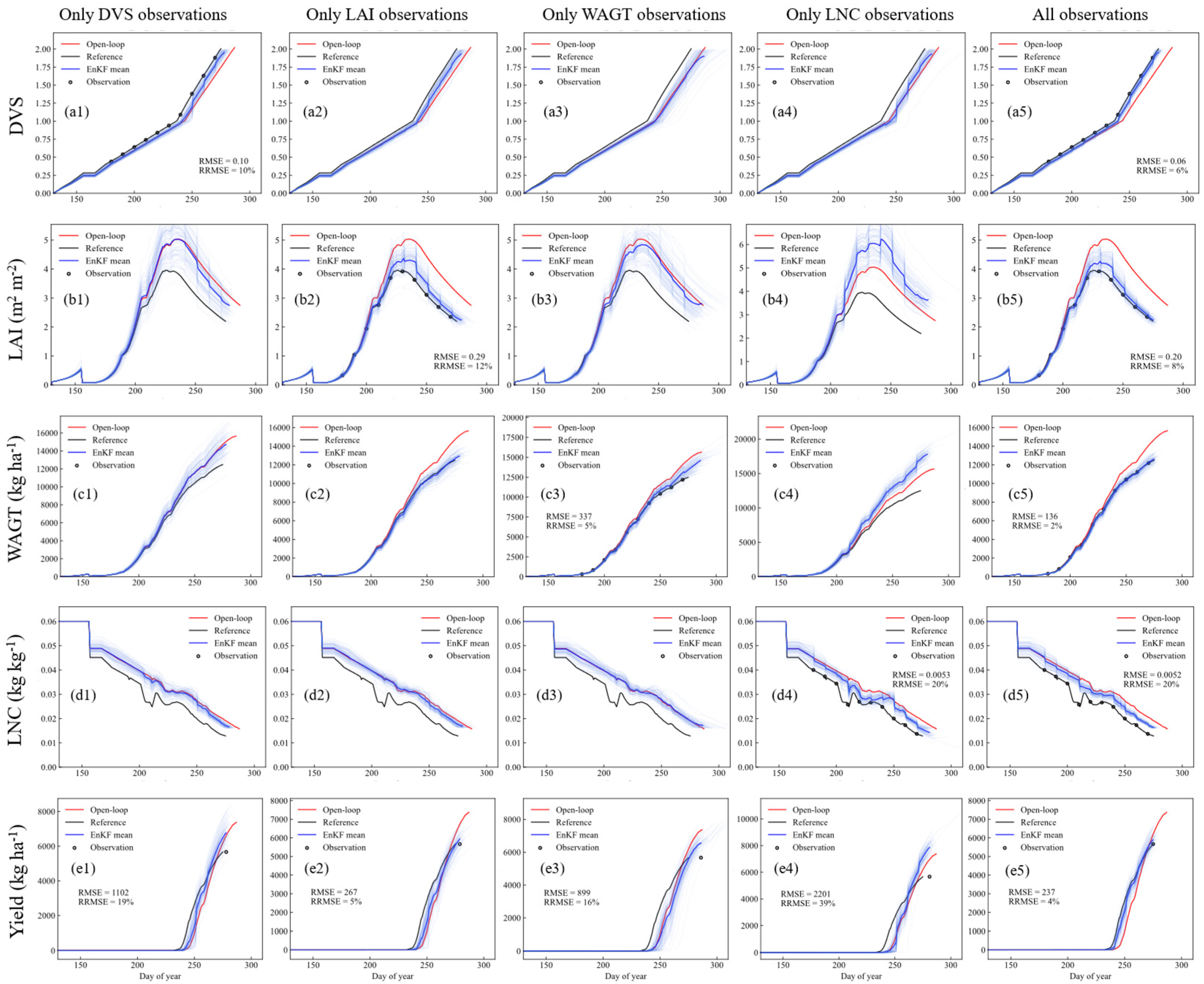
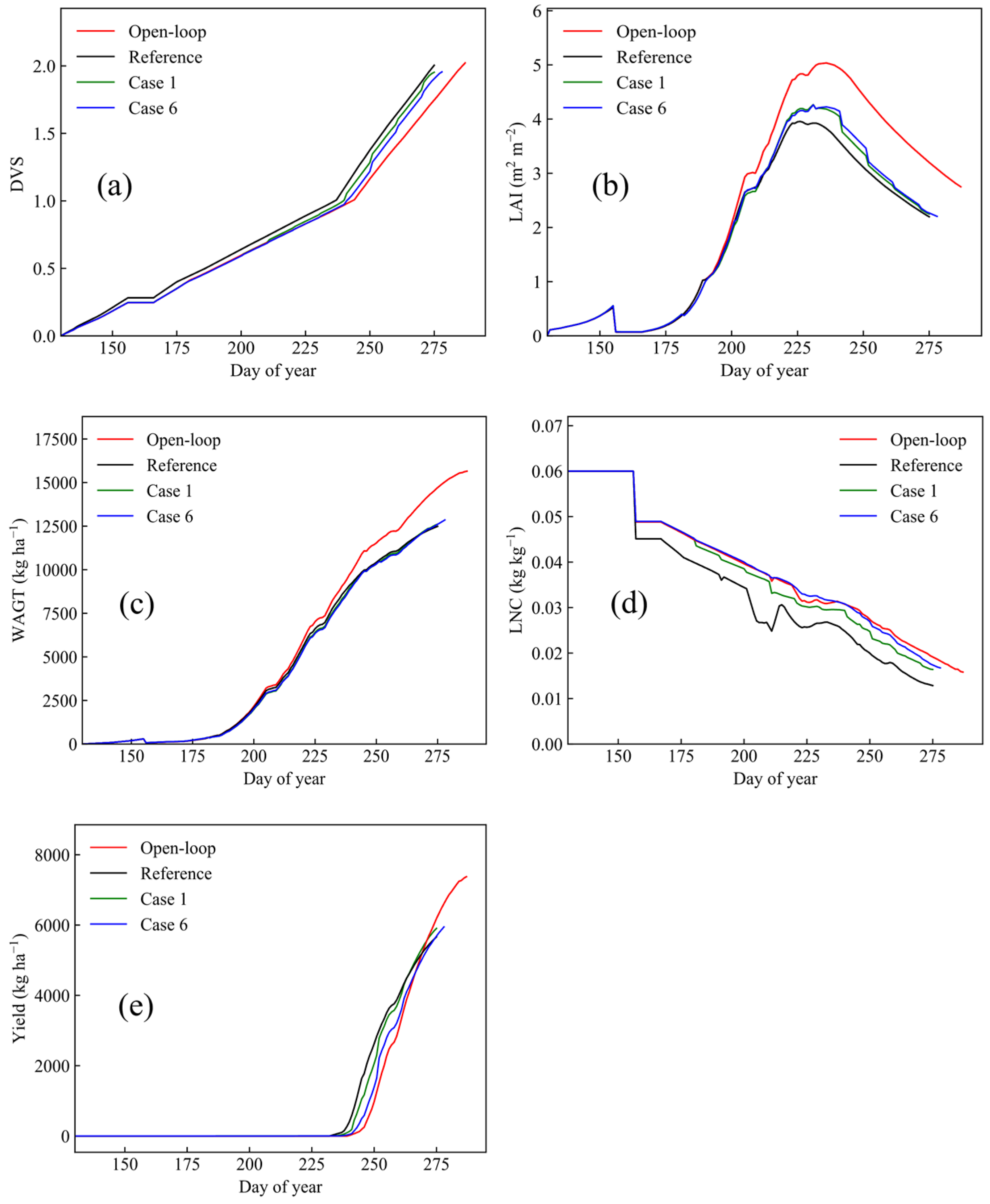
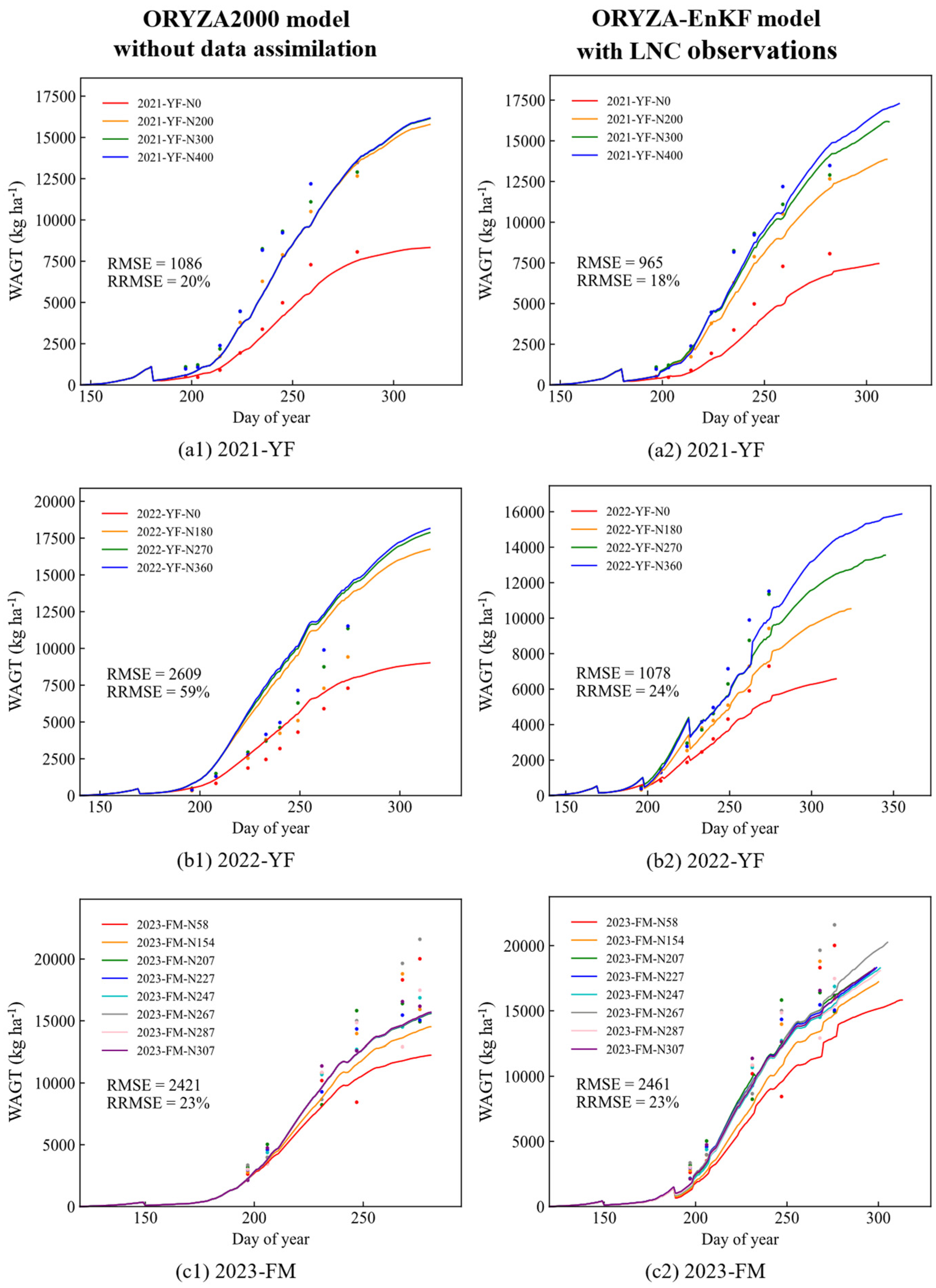
3.3. Value of LNC Observation to ORYZA-EnKF Data Assimilation System

In this section, the OSS was utilized to assess the performance of the ORYZA-EnKF data assimilation system. To investigate the influence of different observation variables on crop model simulations, this study assimilated all observations as well as individual DVS, LAI, WAGT, and LNC observations into the ORYZA2000 model. The results are presented in Figure 5. It can be found that the simulation accuracy of DVS improved after taking DVS observations into account, but the results for other state variables showed no significant enhancement. Assimilating the LAI improved the simulation results of many other state variables, but had a limited impact on the updating of rice LNC (Figure 5(d2)), which suggested that the LAI alone is insufficient to capture the nitrogen dynamics. The simulations of WAGT and yield were also improved when WAGT observations were assimilated into the ORYZA2000 model, mainly because above-ground biomass is the sum of the mass of stems, leaves, and grains of rice. This could be more apparent in crop models that calculate yield using the harvest index [31]. But, the improvements in overall simulation accuracy by taking WAGT observations into account were less effective than the LAI, which is similar to the findings of Zhang et al. [65]. In the ORYZA2000 model, rice yield is not calculated using the harvest index directly but is instead determined through more complex processes of dry matter accumulation and distribution. Compared to WAGT, the LAI could capture more accurate information about leaf growth, transpiration, precipitation interception, plant photosynthesis, and dry matter distribution [25,53].
Incorporating LNC observations into the ORYZA2000 model enhanced the simulation of DVS and LNC, but it failed to capture the dynamics of the LAI, WAGT, and yield, and even worsened the results. This could be explained by the fact that when the crop growth rate decreases due to a reduction in nitrogen supply, leaf growth also declines. Considering that LNC is calculated based on leaf mass, the slowdown in leaf mass growth also results in changes in LNC (Formula (15)). As a consequence, there exists a feedback loop between leaf biomass, the LAI, and LNC [15]. And, the relationship between LNC and crop growth is more intricate and does not exhibit the nearly linear relationship observed in the LAI or WAGT. Although the result suggested that LNC played a crucial role in modeling crop nitrogen processes, relying solely on LNC observations was insufficient to fully capture the overall rice growth status. After adding other observations, the simulation results were significantly improved (Figure 5(a5–e5)).
To further explore the value of nitrogen observations, LNC was excluded from the set of observed variables and compared with the results from assimilating all observed data, as illustrated in Figure 6. This figure shows that the simulation accuracy can be effectively enhanced by incorporating DVS, LAI, and WAGT observations, which aligns with results reported in previous studies [39,53]. However, the data assimilation system failed to capture the dynamic nitrogen processes without nitrogen observations. Even with three other growth states observations, the rice LNC could not be effectively updated. Building on this, assimilating rice LNC with DVS, the LAI, and WAGT together not only enhanced the accuracy of LNC but also improved the rice growth simulations.
It was also observed that the effects of assimilating LNC in the early stages were less pronounced compared to the middle and late stages, which could be related to the dilution process of rice LNC [66,67]. In the OSS experiments, the variance of each observation was set to 10% of its value. For LNC, uncertainty was highest in the early growth stages and decreased in the middle and late stages. When the observation uncertainty was high, the influence of nitrogen observations on model updates was less effective compared to other state variables. As uncertainty decreased over time, assimilating LNC contributed to a significant improvement in model accuracy.

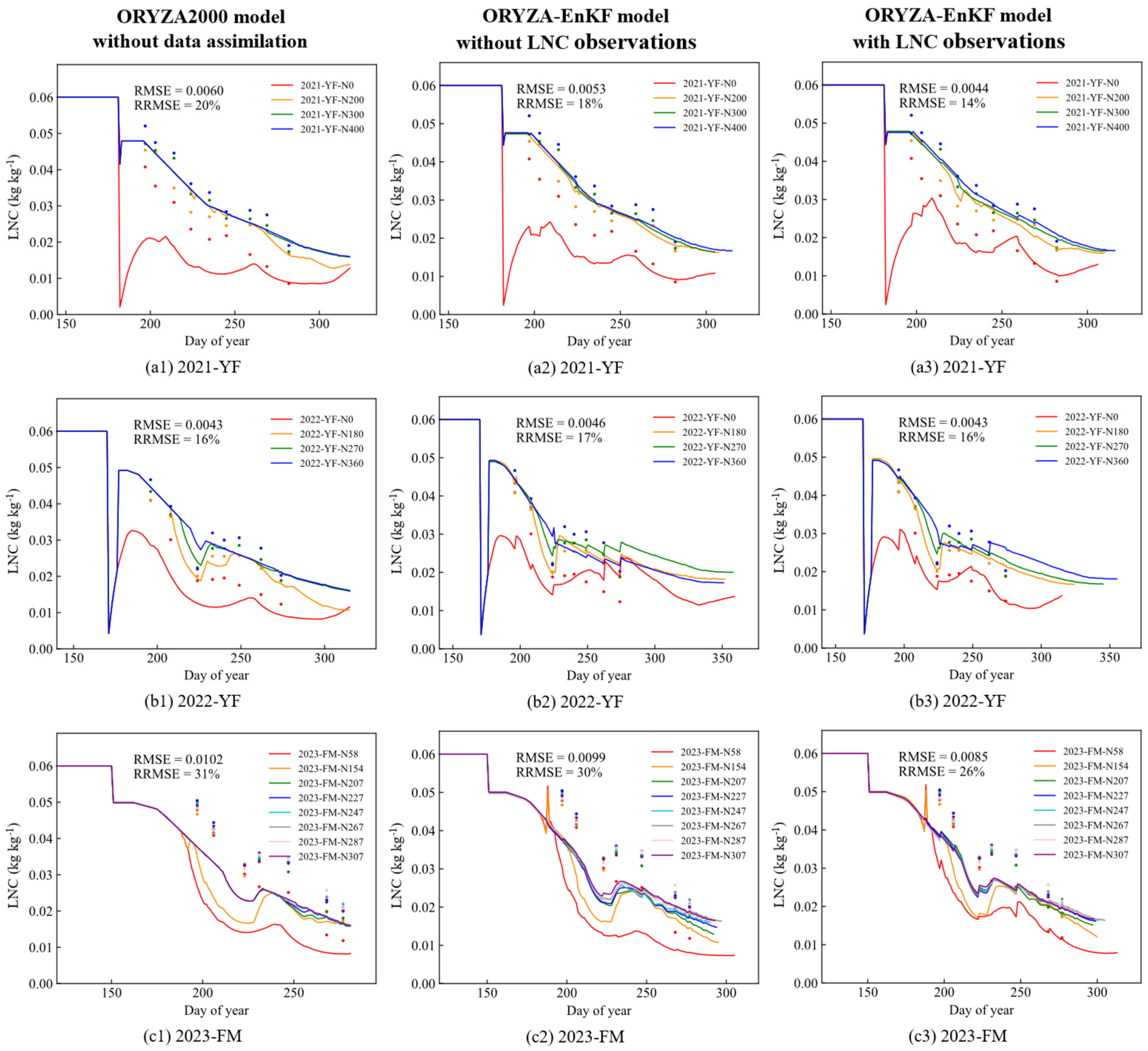
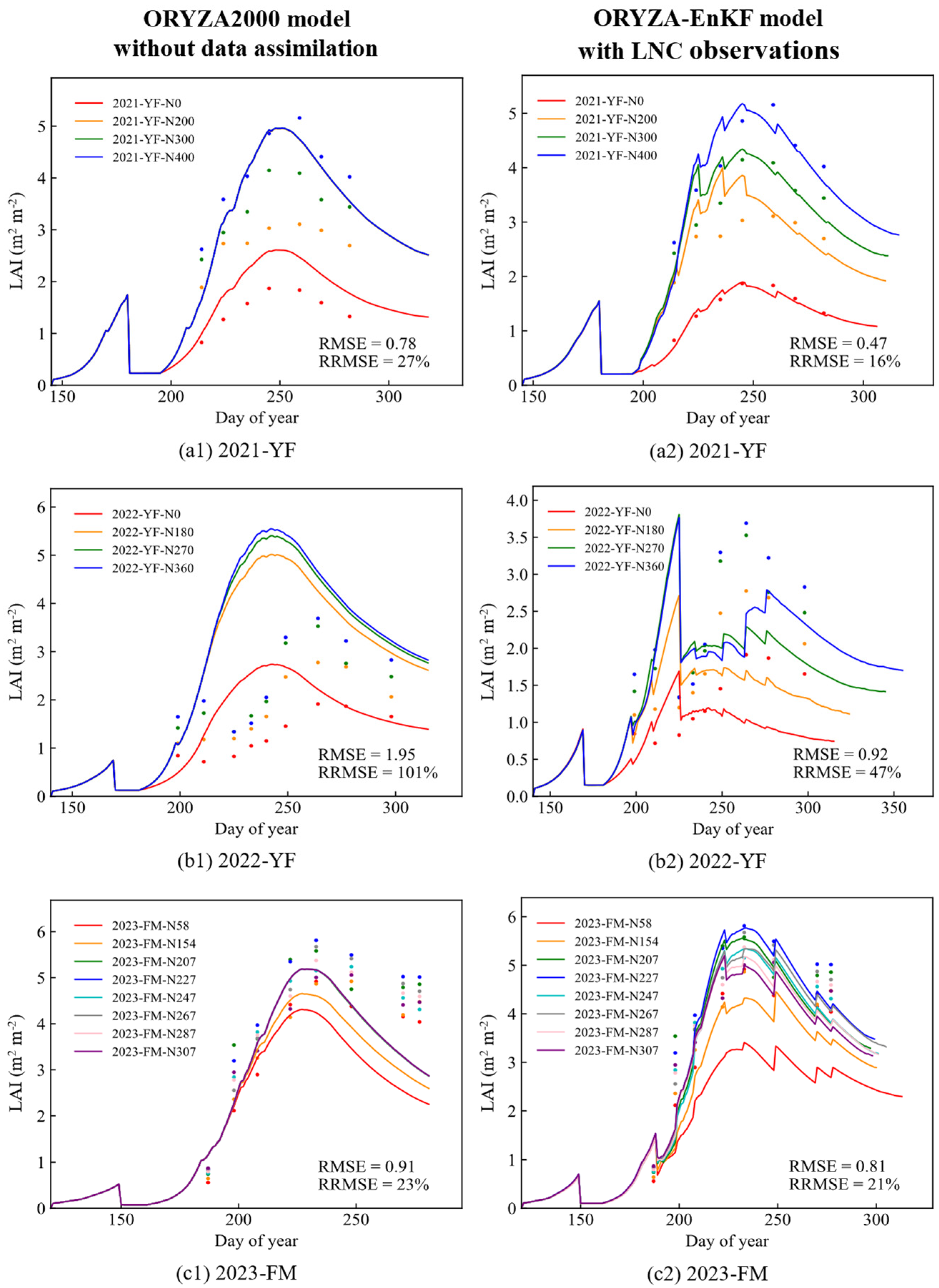
3.4. Test in the Three-Year Experiment

Based on three consecutive years of experimental data, this study tested the ORYZA-EnKF data assimilation system and compared it with deterministic modeling. Four observational variables comprising DVS, the LAI, WAGT, and LNC were selected to be assimilated. To further assess the impact of nitrogen observations on the data assimilation system, comparisons were also made with assimilation results that included all observations except LNC. The RMSE and RRMSE results of DVS, the LAI, WAGT, LNC and yield for the three years are presented in Table 3.
Compared to the original ORYZA2000 model, the ORYZA-EnKF model without LNC observations improved model accuracy in rice DVS, LAI, WAGT, and yield simulations, which indicated that the assimilation of DVS, LAI, and WAGT observations enhanced the understanding of the crop growth processes. However, there were no notable changes in the simulation of LNC. The RMSEs of LNC simulated by the ORYZA-EnKF data assimilation system without LNC observations were 0.0053 kg kg−1, 0.0046 kg kg−1, and 0.0099 kg kg−1, respectively, in the three years. In the absence of nitrogen information, the model failed to effectively capture the nitrogen dynamics. Building on this, the incorporation of LNC observations further improved the accuracy of the simulations for rice growth and nitrogen processes. The RMSE of rice LNC decreased to 0.0044 kg kg−1, 0.0043 kg kg−1, and 0.0085 kg kg−1, and the RRMSE decreased to 14%, 16%, and 26%, respectively, in the three years. By absorbing all four observed variables, yield simulations were also improved. In 2022-YF and 2023-FM, the RMSE of yield estimation decreased from 3484 kg ha−1 and 1869 kg ha−1 to 1430 kg ha−1 and 860 kg ha−1, respectively.
Figure 7 compared the simulation results of three models on rice LNC. In the 2021-YF experiment, the RRMSE of LNC simulated by ORYZA2000 was 20%, but the LNC curves of the N200, N300, and N400 treatments showed no apparent difference in the early and middle growth stages, which were inconsistent with actual observations. Meanwhile, the LNC simulations of the N0 treatment were significantly lower than measured values. After the LNC observations were assimilated into the model, the dynamic LNC simulations under different nitrogen application treatments were improved. Especially in the N0 treatment, the estimated RRMSE was reduced from 41% to 32%. In the simulation of 2022-YF, RRMSE did not decrease and remained at 16%, primarily due to the 10% observation uncertainty in this study and the relatively low error inherent in the ORYZA2000 model. In 2023-FM experiment, the ORYZA-EnKF reduced prediction RRMSE from 31% to 26%. And, the estimation accuracy of N58 was improved significantly, with the RRMSE decreasing from 50% to 41%. The findings of Li et al. [16] also indicated that the ORYZA2000 model had structural errors in its nitrogen processes, often leading to an underestimation of leaf nitrogen content in low-nitrogen treatments. This study demonstrated that data assimilation has the potential to alleviate the structural errors of the ORYZA2000 model, enhancing the accuracy of nitrogen dynamic simulations.
The simulation results of the LAI and WAGT by the ORYZA-EnKF model with LNC observations were compared with those of the ORYZA2000 model. As illustrated in Figure 8 and Figure 9, during the 2022-YF simulation, the ORYZA2000 model demonstrated significant limitations in capturing the dynamic variations of the LAI and WAGT. This is primarily due to the inability of the model to incorporate real-world uncertainties in crop growth, such as the weed issues observed in the 2022-YF experiment. As shown in Figure 8, the LAI did not continue to increase with crop growth on day 225. This stagnation was attributed to inadequate weed management in the 2022-YF trail, resulting in a severe weed infestation that adversely affected rice growth. Although crop growth showed a degree of recovery after the weeds were removed, it remained relatively weak. However, the ORYZA2000 model cannot consider these factors, resulting in inaccurately high simulation results for the LAI and WAGT. After incorporating observations into the crop model, there was a significant improvement in addressing the overestimation of the rice LAI and WAGT, and the differences between various nitrogen treatments were effectively captured. This aligns with the findings of Hu et al. [24], where data assimilation mitigated model uncertainty caused by artificial leaf stripping and enhanced the accuracy of LAI and stem biomass simulations by incorporating LAI observations.
Unlike the monotonically increasing or decreasing (after reaching a peak) patterns seen in DVS, the LAI, and WAGT, LNC generally declines but exhibits dynamic fluctuations due to fertilization practices. Jongschaap [68] found that incorporating a remotely sensed LAI improved crop model accuracy, but adjustments to canopy nitrogen content worsened model predictions. This can be attributed to the relatively weak influence of nitrogen content on other growth variables (such as plant biomass) in crop models. Researchers have modified the nitrogen module of the ORYZA2000 model to address various requirements, yet these adapted models were seldom made publicly available [69,70]. By introducing LNC observations, the ORYZA-EnKF data assimilation system can compensate for certain structural errors in nitrogen processes, and further improve the simulation accuracy of rice growth.

3.5. Potential Applications and Future Work

Previous studies often selected one or two observational variables for data assimilation, primarily constrained by observation and computational costs [20,21]. Therefore, this study proposed a data assimilation system capable of integrating four different types of observations, DVS, the LAI, WAGT, and LNC. By incorporating these variables, which contain diverse types of information about crop growth, the system provided a more comprehensive description of crop growth and nutrient status. With the rapid proliferation of smartphones, RGB images captured by mobile phones has attracted increasing attention from researchers [36,71]. Therefore, future studies can focus on integrating the crop growth status obtained from smartphone images with crop growth models [39]. Considering the reduction in flight costs, the model can also be applied on a larger scale by incorporating extensive observations obtained from UAV images [31,72]. This approach could provide farmers with a low-cost and convenient solution for crop growth assessment and decision-making.

4. Conclusions

This study developed a new ORYZA-EnKF data assimilation system capable of simultaneously incorporating multivariate observations including the rice DVS, LAI, WAGT and LNC. We performed a sensitivity analysis for the ORYZA2000 model and calibrated the model by adjusting the sensitive parameters. Subsequently, the observing simulation system was utilized to explore the values of different observational variables in the data assimilation system. Finally, the ORYZA-EnKF system was tested using data from a three-year field experiment. The results showed that only a few parameters significantly influenced the key state variables of the crop model. By adjusting these parameters, the ORYZA2000 model can achieve a preliminary simulation of rice growth. Assimilating the LAI significantly reduced model uncertainty; absorbing LNC only updated the state of the LNC itself. Integrating observations of DVS, the LAI, and WAGT into the crop model improved the accuracy of crop growth simulations. Furthermore, adding LNC information allowed for a more accurate representation of rice nitrogen dynamics, thereby enhancing the simulation of crop growth and yield formation. In the test of the three-year experiment, the RRMSE for the LAI was reduced from 23–101% to 16–47% compared to the ORYZA2000 model. The RRMSE for LNC simulations decreased from 16–31% to 14–26% across all nitrogen treatments, and the RRMSE decreased from 32–50% to 30–41% under low-nitrogen conditions. By incorporating nitrogen observation data, the ORYZA-EnKF data assimilation system can deal with structural errors in nitrogen processes, particularly under low-nitrogen treatment conditions. This study provides a new insight for precision nitrogen management.

Supplementary Materials

The following supporting information can be downloaded at: https://www.mdpi.com/article/10.3390/agronomy14102402/s1, Table S1: The definition of ORYZA2000 model parameters and their prior values; Figure S1: Sensitivity indices of parameters in ORYZA2000 model for rice LNC at four development stages under N0 scenario; Figure S2: Sensitivity indices of parameters in ORYZA2000 model for rice LNC at four development stages under N200 scenario; Figure S3: Sensitivity indices of parameters in ORYZA2000 model for rice LNC at four development stages under N300 scenario; Figure S4: Sensitivity indices of parameters in ORYZA2000 model for rice LNC at four development stages under N400 scenario; Figure S5: Sensitivity indices of parameters in ORYZA2000 model for rice LAI at four development stages under N0 scenario; Figure S6: Sensitivity indices of parameters in ORYZA2000 model for rice LAI at four development stages under N200 scenario; Figure S7: Sensitivity indices of parameters in ORYZA2000 model for rice LAI at four development stages under N300 scenario; Figure S8: Sensitivity indices of parameters in ORYZA2000 model for rice LAI at four development stages under N400 scenario; Figure S9: Sensitivity indices of parameters in ORYZA2000 model for rice WAGT at four development stages under N0 scenario; Figure S10: Sensitivity indices of parameters in ORYZA2000 model for rice WAGT at four development stages under N200 scenario; Figure S11: Sensitivity indices of parameters in ORYZA2000 model for rice WAGT at four development stages under N300 scenario; Figure S12: Sensitivity indices of parameters in ORYZA2000 model for rice WAGT at four development stages under N400 scenario.

Author Contributions

Conceptualization, J.L., L.S. and J.H.; methodology, J.L., J.H. and X.H.; software, J.L. and J.H.; validation, J.L., L.S., J.H. and X.H.; formal analysis, J.L. and L.S.; investigation, J.L., J.H., X.H. and C.S.; resources, L.S. and S.L.; data curation, J.L., J.H., X.H. and C.S.; writing—original draft preparation, J.L.; writing—review and editing, L.S., J.H. and X.H.; visualization, J.L. and J.H.; supervision, L.S. and S.L.; project administration, L.S.; funding acquisition, L.S. All authors have read and agreed to the published version of the manuscript.

Funding

This research was funded by the National Natural Science Foundation of China (Grants No. 51979200 and No. 52179038) and the Fundamental Research Funds for the Central Universities (Grant No. 2042022kf1051).

Data Availability Statement

The data presented in this study are available on request from the corresponding author.

Acknowledgments

The authors gratefully acknowledge Shanghai Hengsha Agriculture and Forestry Industry Development Co., Ltd. for their support in this experiment.

Conflicts of Interest

The authors declare no conflicts of interest.

References

  1. Yuan, S.; Linquist, B.A.; Wilson, L.T.; Cassman, K.G.; Stuart, A.M.; Pede, V.; Miro, B.; Saito, K.; Agustiani, N.; Aristya, V.E.; et al. Sustainable intensification for a larger global rice bowl. Nat. Commun. 2021, 12, 7163. [Google Scholar] [CrossRef]
  2. Wang, Y.; Wu, W.; Xu, J.; Wang, Y.; Wu, Z.; Liu, H. Expounding the Effect of Harvest Management on Rice (Oryza sativa L.) Yield and Latent Loss Based on the Accurate Measurement of Grain Data. Agronomy 2024, 14, 1346. [Google Scholar] [CrossRef]
  3. Cai, S.; Zhao, X.; Pittelkow, C.M.; Fan, M.; Zhang, X.; Yan, X. Optimal nitrogen rate strategy for sustainable rice production in China. Nature 2023, 615, 73–79. [Google Scholar] [CrossRef]
  4. Xu, J.; Cai, H.; Wang, X.; Ma, C.; Lu, Y.; Ding, Y.; Wang, X.; Chen, H.; Wang, Y.; Saddique, Q. Exploring optimal irrigation and nitrogen fertilization in a winter wheat-summer maize rotation system for improving crop yield and reducing water and nitrogen leaching. Agric. Water Manag. 2020, 228, 105904. [Google Scholar] [CrossRef]
  5. Zhang, X.; Zou, T.; Lassaletta, L.; Mueller, N.D.; Tubiello, F.N.; Lisk, M.D.; Lu, C.; Conant, R.T.; Dorich, C.D.; Gerber, J.; et al. Quantification of global and national nitrogen budgets for crop production. Nat. Food. 2021, 2, 529–540. [Google Scholar] [CrossRef]
  6. Morari, F.; Zanella, V.; Gobbo, S.; Bindi, M.; Sartori, L.; Pasqui, M.; Mosca, G.; Ferrise, R. Coupling proximal sensing, seasonal forecasts and crop modelling to optimize nitrogen variable rate application in durum wheat. Precis. Agric. 2021, 22, 75–98. [Google Scholar] [CrossRef]
  7. Zhao, R.; Ma, Y.; Wu, S. A Review of the Research Status and Prospects of Regional Crop Yield Simulations. Agronomy 2024, 14, 1397. [Google Scholar] [CrossRef]
  8. Yuan, S.; Saito, K.; van Oort, P.A.J.; van Ittersum, M.K.; Peng, S.; Grassini, P. Intensifying rice production to reduce imports and land conversion in Africa. Nat. Commun. 2024, 15, 835. [Google Scholar] [CrossRef]
  9. Asseng, S.; Ewert, F.; Martre, P.; Rötter, R.P.; Lobell, D.B.; Cammarano, D.; Kimball, B.A.; Ottman, M.J.; Wall, G.W.; White, J.W.; et al. Rising temperatures reduce global wheat production. Nat. Clim. Chang. 2015, 5, 143–147. [Google Scholar] [CrossRef]
  10. Wang, B.; Feng, P.; Liu, D.L.; Leary, G.J.O.; Macadam, I.; Waters, C.; Asseng, S.; Cowie, A.; Jiang, T.; Xiao, D.; et al. Sources of uncertainty for wheat yield projections under future climate are site-specific. Nat. Food. 2020, 1, 720–728. [Google Scholar] [CrossRef]
  11. van Oosterom, E.J.; Borrell, A.K.; Chapman, S.C.; Broad, I.J.; Hammer, G.L. Functional dynamics of the nitrogen balance of sorghum: I. N demand of vegetative plant parts. Field Crop. Res. 2010, 115, 19–28. [Google Scholar] [CrossRef]
  12. Soufizadeh, S.; Munaro, E.; McLean, G.; Massignam, A.; van Oosterom, E.J.; Chapman, S.C.; Messina, C.; Cooper, M.; Hammer, G.L. Modelling the nitrogen dynamics of maize crops—Enhancing the APSIM maize model. Eur. J. Agron. 2018, 100, 118–131. [Google Scholar] [CrossRef]
  13. Jing, Q.; Bouman, B.A.M.; Hengsdijk, H.; Van Keulen, H.; Cao, W. Exploring options to combine high yields with high nitrogen use efficiencies in irrigated rice in China. Eur. J. Agron. 2007, 26, 166–177. [Google Scholar] [CrossRef]
  14. Falconnier, G.N.; Corbeels, M.; Boote, K.J.; Affholder, F.; Adam, M.; MacCarthy, D.S.; Ruane, A.C.; Nendel, C.; Whitbread, A.M.; Justes, É.; et al. Modelling climate change impacts on maize yields under low nitrogen input conditions in sub-Saharan Africa. Glob. Chang. Biol. 2020, 26, 5942–5964. [Google Scholar] [CrossRef]
  15. Bouman, B.A.M.; van Laar, H.H. Description and evaluation of the rice growth model ORYZA2000 under nitrogen-limited conditions. Agric. Syst. 2006, 87, 249–273. [Google Scholar] [CrossRef]
  16. Li, T.; Angeles, O.; Marcaida, M.; Manalo, E.; Manalili, M.P.; Radanielson, A.; Mohanty, S. From ORYZA2000 to ORYZA (v3): An improved simulation model for rice in drought and nitrogen-deficient environments. Agric. For. Meteorol. 2017, 237–238, 246–256. [Google Scholar] [CrossRef]
  17. Charney, J.; Halem, M.; Jastrow, R. Use of Incomplete Historical Data to Infer the Present State of the Atmosphere. J. Atmos. Sci. 1969, 26, 1160–1163. [Google Scholar] [CrossRef]
  18. Ines, A.V.M.; Das, N.N.; Hansen, J.W.; Njoku, E.G. Assimilation of remotely sensed soil moisture and vegetation with a crop simulation model for maize yield prediction. Remote Sens. Environ. 2013, 138, 149–164. [Google Scholar] [CrossRef]
  19. Huang, J.; Gómez-Dans, J.L.; Huang, H.; Ma, H.; Wu, Q.; Lewis, P.E.; Liang, S.; Chen, Z.; Xue, J.; Wu, Y.; et al. Assimilation of remote sensing into crop growth models: Current status and perspectives. Agric. For. Meteorol. 2019, 276–277, 107609. [Google Scholar] [CrossRef]
  20. Jin, X.; Kumar, L.; Li, Z.; Feng, H.; Xu, X.; Yang, G.; Wang, J. A review of data assimilation of remote sensing and crop models. Eur. J. Agron. 2018, 92, 141–152. [Google Scholar] [CrossRef]
  21. Luo, L.; Sun, S.; Xue, J.; Gao, Z.; Zhao, J.; Yin, Y.; Gao, F.; Luan, X. Crop yield estimation based on assimilation of crop models and remote sensing data: A systematic evaluation. Agric. Syst. 2023, 210, 103711. [Google Scholar] [CrossRef]
  22. Evensen, G. Sequential data assimilation with a nonlinear quasi-geostrophic model using Monte Carlo methods to forecast error statistics. J. Geophys. Res. Oceans 1994, 99, 10143–10162. [Google Scholar] [CrossRef]
  23. de Wit, A.J.W.; van Diepen, C.A. Crop model data assimilation with the Ensemble Kalman filter for improving regional crop yield forecasts. Agric. For. Meteorol. 2007, 146, 38–56. [Google Scholar] [CrossRef]
  24. Hu, S.; Shi, L.; Huang, K.; Zha, Y.; Hu, X.; Ye, H.; Yang, Q. Improvement of sugarcane crop simulation by SWAP-WOFOST model via data assimilation. Field Crop. Res. 2019, 232, 49–61. [Google Scholar] [CrossRef]
  25. Yang, C.; Lei, H. Evaluation of data assimilation strategies on improving the performance of crop modeling based on a novel evapotranspiration assimilation framework. Agric. For. Meteorol. 2024, 346, 109882. [Google Scholar] [CrossRef]
  26. Wang, Y.; Zhou, H.; Ma, X.; Liu, H. Combining Data Assimilation with Machine Learning to Predict the Regional Daily Leaf Area Index of Summer Maize (Zea mays L.). Agronomy 2023, 13, 2688. [Google Scholar] [CrossRef]
  27. Chen, Y.; Zhang, Z.; Tao, F. Improving regional winter wheat yield estimation through assimilation of phenology and leaf area index from remote sensing data. Eur. J. Agron. 2018, 101, 163–173. [Google Scholar] [CrossRef]
  28. Jin, X.; Li, Z.; Feng, H.; Ren, Z.; Li, S. Estimation of maize yield by assimilating biomass and canopy cover derived from hyperspectral data into the AquaCrop model. Agric. Water Manag. 2020, 227, 105846. [Google Scholar] [CrossRef]
  29. Zhang, Z.; Li, Z.; Chen, Y.; Zhang, L.; Tao, F. Improving regional wheat yields estimations by multi-step-assimilating of a crop model with multi-source data. Agric. For. Meteorol. 2020, 290, 107993. [Google Scholar] [CrossRef]
  30. Yu, D.; Zha, Y.; Shi, L.; Ye, H.; Zhang, Y. Improving sugarcane growth simulations by integrating multi-source observations into a crop model. Eur. J. Agron. 2022, 132, 126410. [Google Scholar] [CrossRef]
  31. Yang, Q.; Shi, L.; Han, J.; Zha, Y.; Yu, J.; Wu, W.; Huang, K. Regulating the time of the crop model clock: A data assimilation framework for regions with high phenological heterogeneity. Field Crop. Res. 2023, 293, 108847. [Google Scholar] [CrossRef]
  32. Liang, H.; Gao, S.; Hu, K. Global sensitivity and uncertainty analysis of the dynamic simulation of crop N uptake by using various N dilution curve approaches. Eur. J. Agron. 2020, 116, 126044. [Google Scholar] [CrossRef]
  33. Li, Z.; Jin, X.; Zhao, C.; Wang, J.; Xu, X.; Yang, G.; Li, C.; Shen, J. Estimating wheat yield and quality by coupling the DSSAT-CERES model and proximal remote sensing. Eur. J. Agron. 2015, 71, 53–62. [Google Scholar] [CrossRef]
  34. Weiss, M.; Jacob, F.; Duveiller, G. Remote sensing for agricultural applications: A meta-review. Remote Sens. Environ. 2020, 236, 111402. [Google Scholar] [CrossRef]
  35. Berger, K.; Verrelst, J.; Féret, J.; Wang, Z.; Wocher, M.; Strathmann, M.; Danner, M.; Mauser, W.; Hank, T. Crop nitrogen monitoring: Recent progress and principal developments in the context of imaging spectroscopy missions. Remote Sens. Environ. 2020, 242, 111758. [Google Scholar] [CrossRef]
  36. Li, J.; Shi, L.; Mo, X.; Hu, X.; Su, C.; Han, J.; Deng, X.; Du, S.; Li, S. Self-correcting deep learning for estimating rice leaf nitrogen concentration with mobile phone images. Comput. Electron. Agric. 2024, 227, 109497. [Google Scholar] [CrossRef]
  37. Wang, W.; Rong, Y.; Zhang, C.; Wang, C.; Huo, Z. Data assimilation of soil moisture and leaf area index effectively improves the simulation accuracy of water and carbon fluxes in coupled farmland hydrological model. Agric. Water Manag. 2024, 291, 108646. [Google Scholar] [CrossRef]
  38. Lancashire, P.D.; Bleiholder, H.; Boom, T.V.D.; Langelüddeke, P.; Stauss, R.; Weber, E.; Witzenberger, A. A uniform decimal code for growth stages of crops and weeds. Ann. Appl. Biol. 1991, 119, 561–601. [Google Scholar] [CrossRef]
  39. Han, J.; Shi, L.; Yang, Q.; Chen, Z.; Yu, J.; Zha, Y. Rice yield estimation using a CNN-based image-driven data as-similation framework. Field Crops Res. 2022, 288, 108693. [Google Scholar] [CrossRef]
  40. Jung, S.; Rickert, D.A.; Deak, N.A.; Aldin, E.D.; Recknor, J.; Johnson, L.A.; Murphy, P.A. Comparison of Kjeldahl and Dumas methods for determining protein contents of soybean products. J. Am. Oil Chem. Society. 2003, 80, 1169–1173. [Google Scholar] [CrossRef]
  41. Beljkaš, B.; Matić, J.; Milovanović, I.; Jovanov, P.; Mišan, A.; Šarić, L. Rapid method for determination of protein content in cereals and oilseeds: Validation, measurement uncertainty and comparison with the Kjeldahl method. Accredit. Qual. Assur. 2010, 15, 555–561. [Google Scholar] [CrossRef]
  42. Aguirre, J. Important Topics Related to the Kjeldahl Method. In The Kjeldahl Method: 140 Years; Aguirre, J., Ed.; Springer: Cham, Switzerland, 2023; pp. 123–145. [Google Scholar]
  43. Bouman, B. ORYZA2000: Modeling Lowland Rice; IRRI: Los Baños, Philippines, 2001. [Google Scholar]
  44. Yadav, S.; Li, T.; Humphreys, E.; Gill, G.; Kukal, S.S. Evaluation and application of ORYZA2000 for irrigation scheduling of puddled transplanted rice in North West India. Field Crop. Res. 2011, 122, 104–117. [Google Scholar] [CrossRef]
  45. Kawakita, S.; Yamasaki, M.; Teratani, R.; Yabe, S.; Kajiya-Kanegae, H.; Yoshida, H.; Fushimi, E.; Nakagawa, H. Dual ensemble approach to predict rice heading date by integrating multiple rice phenology models and machine learning-based genetic parameter regression models. Agric. For. Meteorol. 2024, 344, 109821. [Google Scholar] [CrossRef]
  46. Chapagain, R.; Remenyi, T.A.; Harris, R.M.B.; Mohammed, C.L.; Huth, N.; Wallach, D.; Rezaei, E.E.; Ojeda, J.J. Decomposing crop model uncertainty: A systematic review. Field Crop. Res. 2022, 279, 108448. [Google Scholar] [CrossRef]
  47. Tan, J.; Cui, Y.; Luo, Y. Assessment of uncertainty and sensitivity analyses for ORYZA model under different ranges of parameter variation. Eur. J. Agron. 2017, 91, 54–62. [Google Scholar] [CrossRef]
  48. Li, P.; Ren, L. Evaluating the effects of limited irrigation on crop water productivity and reducing deep groundwater exploitation in the North China Plain using an agro-hydrological model: I. Parameter sensitivity analysis, calibration and model validation. J. Hydrol. 2019, 574, 497–516. [Google Scholar] [CrossRef]
  49. Sobol’, I.M. On sensitivity estimation for nonlinear mathematical models. Mat. Model. 1990, 2, 112–118. [Google Scholar]
  50. Thorp, K.R.; DeJonge, K.C.; Marek, G.W.; Evett, S.R. Comparison of evapotranspiration methods in the DSSAT Cropping System Model: I. Global sensitivity analysis. Comput. Electron. Agric. 2020, 177, 105658. [Google Scholar] [CrossRef]
  51. Yu, J.; Shi, L.; Han, J.; Yang, Q.; Huang, J.; Ye, M. Assessing parametric and nitrogen fertilizer input uncertainties in the ORYZA_V3 model predictions. Agron. J. 2021, 113, 4965–4981. [Google Scholar] [CrossRef]
  52. Tan, J.; Cui, Y.; Luo, Y. Global sensitivity analysis of outputs over rice-growth process in ORYZA model. Environ. Modell. Softw. 2016, 83, 36–46. [Google Scholar] [CrossRef]
  53. Hu, S.; Shi, L.; Zha, Y.; Williams, M.; Lin, L. Simultaneous state-parameter estimation supports the evaluation of data assimilation performance and measurement design for soil-water-atmosphere-plant system. J. Hydrol. 2017, 555, 812–831. [Google Scholar] [CrossRef]
  54. Curnel, Y.; de Wit, A.J.W.; Duveiller, G.; Defourny, P. Potential performances of remotely sensed LAI assimilation in WOFOST model based on an OSS Experiment. Agric. For. Meteorol. 2011, 151, 1843–1855. [Google Scholar] [CrossRef]
  55. Lu, Y.; Chibarabada, T.P.; Ziliani, M.G.; Onema, J.K.; McCabe, M.F.; Sheffield, J. Assimilation of soil moisture and canopy cover data improves maize simulation using an under-calibrated crop model. Agric. Water Manag. 2021, 252, 106884. [Google Scholar] [CrossRef]
  56. Gitelson, A.; Arkebauer, T.; Viña, A.; Skakun, S.; Inoue, Y. Evaluating plant photosynthetic traits via absorption coefficient in the photosynthetically active radiation region. Remote Sens. Environ. 2021, 258, 112401. [Google Scholar] [CrossRef]
  57. Yu, Q.; Cui, Y.; Liu, L. Assessment of the parameter sensitivity for the ORYZA model at the regional scale—A case study in the Yangtze River Basin. Environ. Modell. Softw. 2023, 159, 105575. [Google Scholar] [CrossRef]
  58. Hyun, S.; Yang, S.M.; Kim, J.; Kim, K.S.; Shin, J.H.; Lee, S.M.; Lee, B.; Beresford, R.M.; Fleisher, D.H. Development of a mobile computing framework to aid decision-making on organic fertilizer management using a crop growth model. Comput. Electron. Agric. 2021, 181, 105936. [Google Scholar] [CrossRef]
  59. Liu, J.; Liu, Z.; Zhu, A.; Shen, F.; Lei, Q.; Duan, Z. Global sensitivity analysis of the APSIM-Oryza rice growth model under different environmental conditions. Sci. Total Environ. 2019, 651, 953–968. [Google Scholar] [CrossRef]
  60. Zhao, B.; Ata-Ul-Karim, S.T.; Liu, Z.; Ning, D.; Xiao, J.; Liu, Z.; Qin, A.; Nan, J.; Duan, A. Development of a critical nitrogen dilution curve based on leaf dry matter for summer maize. Field Crop. Res. 2017, 208, 60–68. [Google Scholar] [CrossRef]
  61. Espe, M.B.; Yang, H.; Cassman, K.G.; Guilpart, N.; Sharifi, H.; Linquist, B.A. Estimating yield potential in temper-ate high-yielding, direct-seeded US rice production systems. Field Crop. Res. 2016, 193, 123–132. [Google Scholar] [CrossRef]
  62. Li, T.; Raman, A.K.; Marcaida, M.; Kumar, A.; Angeles, O.; Radanielson, A.M. Simulation of genotype performances across a larger number of environments for rice breeding using ORYZA2000. Field Crops Res. 2013, 149, 312–321. [Google Scholar] [CrossRef]
  63. Gao, Y.; Xu, X.; Sun, C.; Ding, S.; Huo, Z.; Huang, G. Parameterization and modeling of paddy rice (Oryza sativa L. ssp. japonica) growth and water use in cold regions: Yield and water-saving analysis. Agric. Water Manag. 2021, 250, 106864. [Google Scholar] [CrossRef]
  64. Seidel, S.J.; Palosuo, T.; Thorburn, P.; Wallach, D. Towards improved calibration of crop models—Where are we now and where should we go? Eur. J. Agron. 2018, 94, 25–35. [Google Scholar] [CrossRef]
  65. Zhang, C.; Liu, J.; Shang, J.; Dong, T.; Tang, M.; Feng, S.; Cai, H. Improving winter wheat biomass and evapotran-spiration simulation by assimilating leaf area index from spectral information into a crop growth model. Agric. Water Manag. 2021, 255, 107057. [Google Scholar] [CrossRef]
  66. Ata-Ul-Karim, S.T.; Yao, X.; Liu, X.; Cao, W.; Zhu, Y. Development of critical nitrogen dilution curve of Japonica rice in Yangtze River Reaches. Field Crops Res. 2013, 149, 149–158. [Google Scholar] [CrossRef]
  67. Qiu, Z.; Ma, F.; Li, Z.; Xu, X.; Ge, H.; Du, C. Estimation of nitrogen nutrition index in rice from UAV RGB images coupled with machine learning algorithms. Comput. Electron. Agric. 2021, 189, 106421. [Google Scholar] [CrossRef]
  68. Jongschaap, R.E.E. Run-time calibration of simulation models by integrating remote sensing estimates of leaf area index and canopy nitrogen. Eur. J. Agron. 2006, 24, 316–324. [Google Scholar] [CrossRef]
  69. Yu, Q.; Cui, Y. Improvement and testing of ORYZA model water balance modules for alternate wetting and drying irrigation. Agric. Water Manag. 2022, 271, 107802. [Google Scholar] [CrossRef]
  70. Gao, Y.; Sun, C.; Ramos, T.B.; Huo, Z.; Huang, G.; Xu, X. Modeling nitrogen dynamics and biomass production in rice paddy fields of cold regions with the ORYZA-N model. Ecol. Model. 2023, 475, 110184. [Google Scholar] [CrossRef]
  71. Mendes, J.; Pinho, T.M.; Neves Dos Santos, F.; Sousa, J.J.; Peres, E.; Boaventura-Cunha, J.; Cunha, M.; Morais, R. Smartphone Applications Targeting Precision Agriculture Practices—A Systematic Review. Agronomy 2020, 10, 855. [Google Scholar] [CrossRef]
  72. Yu, D.; Zha, Y.; Shi, L.; Jin, X.; Hu, S.; Yang, Q.; Huang, K.; Zeng, W. Improvement of sugarcane yield estimation by assimilating UAV-derived plant height observations. Eur. J. Agron. 2020, 121, 126159. [Google Scholar] [CrossRef]
Figure 1. Flowchart of the construction of the ORYZA-EnKF data assimilation system.
Agronomy 14 02402 g001
Figure 2. (a) Location of Hengsha township, Shanghai city in China; (b) Location of two experiment sites (Yongfa village and Fumin village) in Hengsha Township; (c) Overview of 12 experimental plots in Yongfa village; (d) Overview of 24 experimental plots in Fumin village.
Agronomy 14 02402 g002
Figure 4. Simulation results of rice state variables for three years by ORYZA2000 model. (a1a3) DVS simulation results for 2021, 2022, and 2023; (b1b3) LAI simulation results for 2021, 2022, and 2023; (c1c3) WAGT simulation results for 2021, 2022, and 2023; (d1d3) LNC simulation results for 2021, 2022, and 2023; and (e1e3) Yield simulation results for 2021, 2022, and 2023.
Agronomy 14 02402 g004
Figure 5. Influence of different observed variables on the ORYZA-EnKF data assimilation system. (a1e1) Simulation results for DVS, LAI, WAGT, LNC, and yield when only DVS observations were assimilated; (a2e2) Results when only LAI observations were assimilated; (a3e3) Results when only WAGT observations were assimilated; (a4e4) Results when only LNC observations were assimilated; and (a5e5) Results when all observations were assimilated. The different columns represent the observations assimilated by ORYZA-EnKF, and the different rows are the simulation results of the model state variables. The black dots and lines refer to OSS observations; the red lines are open-loop simulation results; the thin lines in light blue are the simulation results of the different samples, and the thick lines in blue are the averages of the samples.
Agronomy 14 02402 g005
Figure 6. Effects of nitrogen observation on the ORYZA-EnKF data assimilation system. (ae) represent the simulation results for DVS, LAI, WAGT, LNC, and yield, respectively. The black dots and lines refer to OSS observations; the red lines are open-loop simulation results; the green line in Case 1 is the simulation result of all observed variables, and the blue line in Case 6 represents the result of removing the observation of leaf nitrogen content from all observed variables.
Agronomy 14 02402 g006
Figure 7. Simulation of rice LNC by the ORYZA-EnKF data assimilation system. The legend is labeled with year + test field location + nitrogen application level. (a1a3) 2021-YF; (b1b3) 2022-YF; (c1c3) 2023-FM.
Agronomy 14 02402 g007
Figure 8. Simulation of the rice LAI by the ORYZA-EnKF data assimilation system. The legend is labeled with year + test field location + nitrogen application level. (a1,a2) 2021-YF; (b1,b2) 2022-YF; (c1,c2) 2023-FM.
Agronomy 14 02402 g008
Figure 9. Simulation of WAGT by the ORYZA-EnKF data assimilation system. The legend is labeled with year + test field location + nitrogen application level. (a1,a2) 2021-YF; (b1,b2) 2022-YF; (c1,c2) 2023-FM.
Agronomy 14 02402 g009
Table 1. Details of the rice field experiments.
YearLocationVarietyNumber of PlotsN application Rate
(kg N ha−1)
2021Yongfa VillageNJ4612N0, N200, N300, N400
2022Yongfa VillageNJ4612N0, N180, N270, N360
2023Fumin VillageCXJ20124N58, N154, N207, N227,
N247, N267, N287, N307
Table 2. Evaluation of the simulated accuracy of state variables by the ORYZA2000 model.
VariableUnitDatasetNumber of
Observations
RMSERRMSE
DVS-Calibration80.087%
Validation40.1619%
LAIm2 m−2Calibration641.5565%
Validation640.9123%
WAGTkg ha−1Calibration64199840%
Validation48242123%
LNCkg kg−1Calibration680.005318%
Validation560.010231%
Yieldkg ha−1Calibration8250840%
Validation8186922%
Table 3. Simulation results of the ORYZA-EnKF system in rice experiments of three years.
State
Variable
Experiment
Name
Number of
Observations
ORYZA2000 Model
without
Data Assimilation
ORYZA-EnKF Model
without
LNC Observations
ORYZA-EnKF Model with LNC
Observations
RMSERRMSERMSERRMSERMSERRMSE
DVS2021-YF40.109%0.076%0.087%
2022-YF40.054%0.2726%0.1514%
2023-FM40.1619%0.098%0.109%
LAI2021-YF280.7827%0.4716%0.4716%
2022-YF361.95101%0.9248%0.9247%
2023-FM640.9123%0.7519%0.8121%
WAGT2021-YF32108620%99218%96518%
2022-YF32260959%122428%107824%
2023-FM48242123%240422%246123%
LNC2021-YF360.006020%0.005318%0.004414%
2022-YF320.004316%0.004617%0.004316%
2023-FM560.010231%0.009930%0.008526%
Yield2021-YF46609%99313%79411%
2022-YF4348470%133927%143029%
2023-FM8186922%102012%86010%
Disclaimer/Publisher’s Note: The statements, opinions and data contained in all publications are solely those of the individual author(s) and contributor(s) and not of MDPI and/or the editor(s). MDPI and/or the editor(s) disclaim responsibility for any injury to people or property resulting from any ideas, methods, instructions or products referred to in the content.

