Calibration and Modeling of Parameters for Kale Root Stubble Simulation Based on the Discrete Unit Method

Abstract

Today, the post-harvest root stubble treatment of kale in Hunan mostly uses manual pulling and centralized treatments, which are inefficient and labor-intensive. In this study, to realize the direct mechanical crushing of kale root stubble and return it to the field after harvesting, we established an accurate simulation model of kale root stubble by creating a model of the root stubble of kale and calibrating the parameters of the simulation. This study took Jingfeng No. 1 kale stubble as the research object and used EDEM2021.2 simulation software to study the parameters of the kale stubble-crushing simulation model. The peak shear force of the sheared kale root stubble was used as the test data, and the most significant factors affecting the shear force were screened out through the Plackett–Burman test for the Design-Expert design. In addition, the steepest climb test and Box–Behnken test were used to accurately assess the factor data to obtain the best simulation value, which was 861.02 N. The relative error between the simulated and measured values was 0.61%. Finally, an accurate simulation stubble model was established by combining the best simulation parameters with the measured stubble length and diameter. This model provides a theoretical basis and technical support for more in-depth research on stubble simulation and mechanized stubble return.

1. Introduction

Today, China’s kale-dominant production areas can be divided into four major production areas: the northern kale-dominant area, the middle and lower reaches of the Yangtze River, the southwest kale-dominant area, and the South China kale-dominant area. Among them, the kale-dominant area in the middle and lower reaches of the Yangtze River encompasses about 4.4 million mu (293,000 hm²) of sown land, accounting for about 31% of the total area of the country. Here, the varieties are mainly flat-ball and oxheart types, with the area of round-ball types increasing each year [1]. However, the region is still plagued by problems such as degradation of arable land, waste of resources, ecological damage, environmental pollution, serious disasters, and small scale. It is still impossible to use large-scale agricultural machinery in large quantities, and the problem of stubble in the soil after harvesting kale in the region is serious, with most of it having to be pulled out manually, which is a waste of manpower and an underutilization of resources. Growing kale in successive seasons induces cruciferous rhizomatosis, which is characterized by abnormal tumorous swelling of the infected root system, leading to reduced drought resistance and inadequate nutrient distribution and resulting in reduced crop yields. Cruciferous rhizomatosis is one of the most damaging diseases in cruciferous crops worldwide [2]. Therefore, most kale is grown under rotation in Hunan, which makes it feasible to return kale root stubble directly to the field after harvest. However, kale root stubble cannot rot quickly if returned to the field without treatment, resulting in nutrients not being absorbed by the soil. Thus, after harvest, the root stubble can be directly returned to the field using mechanical crushing and rototilling, which can make full use of the root stubble’s nutrients and is not labor intensive. Based on the above cultivation methods and kale stubble characteristics, the establishment of a suitable kale stubble model and the calibration of its simulation parameters are conducive to the study and optimization of the problems that will arise in the actual process of kale stubble crushing and returning to the field.

The discrete unit method is widely used in crop root and straw calibration, and some scholars have achieved more results. Using discrete element method modeling software, Zhao Jikun et al. developed a discrete element mechanical model of rice straw and calibrated the model parameters [3]. Nona et al. developed a physical parameter model to describe the compression properties of wheat straw and hay using compression tests [4]. The friction coefficient, normal stiffness, and tangential stiffness of the crops were calibrated using different shear test parameters with a relative error of less than 2% [5]. Fang used the stacking angle test to calibrate the simulation parameters for the static and rolling friction coefficients with an average relative error of only 0.29% [6]. To improve the accuracy of the simulation results of maize straw, Tong Shihe et al. proposed a method to build a refined simulation model of maize straw based on the discrete element method (DEM) to construct simulation models of stalked and unstalked straw [7]. Schramm et al. used EDEM to calibrate the modulus of elasticity and Poisson’s ratio of wheat straw in a three-point bending simulation test and a uniaxial compression simulation test; the relative error with the physical test results was only 3.11% [8]. To solve the lack of accurate models available for the discrete element modeling of rice clearing material clogging and improve the accuracy of the parameters used in discrete element modeling and simulation studies of rice plants, Hou J et al. used the Plackett–Burman, Central Composite, and Box–Behnken test methods based on the discrete element HBP simulation model parameters and bonding parameters for discrete element simulation calibration and the discrete element modeling of rice plants to provide a parametric basis for discrete element simulation studies [9]. In order to obtain the discrete elemental simulation parameters of straw biochar, Yawen Zhang et al. used a combination of simulation analysis and physical tests to calibrate the contact parameters of biochar. Three significant parameters in the discrete element simulation parameters of straw biochar were finally determined by the Plackett–Burman test, the steepest climb test, and the Box–Behnken test. Comparison of the stack angle test with its Rocky discrete element simulation results showed that the error of the determined parameters was 2.0% and the error of the determined parameters was 3.0%. The determined parameter error is only 2.33% [10]. Maraldi M et al. conducted compression tests on rice straw and analyzed the relationship between the mechanical properties, such as Poisson’s ratio and elastic modulus, and the geometry and density of rice straw after baling [11]. Using a discrete element model, Wenhang Liu et al. established bonded particle models of epidermis–epidermis, internal flesh–internal flesh, and epidermis–internal flesh based on the Hertz–Mindlin model. Then, physical tests and simulation optimization design methods were combined to validate the discrete element model and verify the feasibility of the discrete element model for simulation analysis [12]. Based on the experimental results of the physical stacking angle of moso bamboo Phyllostachys edulis powder, Dong Liu et al. used a combination of discrete element method (DEM) simulation and design of experiments (DOE) to obtain the quadratic regression model of the contact parameters between the stacking angle of the bamboo powder and the simulation parameters by using the Plackett–Burman (P-BD) experiments, the slope-climbing experiments, and the response surface experiments. The polynomial regression model and the optimal combination of contact parameters were predicted using the physical stacking angle as the target value. The DEM calibration method of this study can provide a reference for the subsequent development of material models for assessing the kinematic behavior of biomass particles and their interaction with equipment [13]. Zhang Tao et al. used the relative error value of the radial stacking angle as an evaluation index to calibrate the contact parameters of corn straw and kneader hammer, corn straw, and corn stover; the relative error between the true results and the experimental results was 8.127% [14]. The discrete unit method can simulate the microstructure and interaction forces of the root stubble, so it can obtain higher accuracy simulation results and simulate the movement and deformation of the root stubble, which is of great significance for the study of its mechanical properties. Kale, as an important agricultural crop in China, is widely grown throughout the country. Kale likes a humid climate but does not like heat. The optimum temperature for kale growth is 10–20 °C. In addition, kale does not tolerate drought and water damage and requires a loose, fertile soil type. Therefore, kale is widely grown in central and southern China. Most of kale’s post-harvest treatment involves manual plucking or plucking and concentrated composting. In some areas, kale is mechanically shredded and returned to the field. In this paper, the discrete unit method is used to establish a kale root particle model, and the Hertz–Mindlin with bonding V2 contact model is used to determine parameters such as kale bonding stiffness and the ultimate stress shear modulus through kale root shear damage tests and response surface tests. The results provide reference values for the discrete element modeling method of kale roots or kale simulation mechanical tests.

2. Materials and Methods

2.1. Shear Test

2.1.1. Shear Test Purpose and Method

A shear test was conducted on the lower end of kale root stubble using a universal mechanical testing machine to obtain the peak shear force required to shear the lower end of the kale root. The data were used to provide a reference for discrete element modeling of the kale root stubble. Then, the steepest climb test and response surface test were used to obtain the optimal values for the contact radius and normal stiffness per unit area required for the modeling of the kale root stubble, which will provide a reference for the subsequent related kale root-crushing simulation study. The calibration process is shown in Figure 1. The shear test was carried out using a universal mechanical testing machine on the lower end of 50 Jingfeng No. 1 kale roots. After measuring and counting, 52% of the diameters on the end of the kale stubble were in the range of 23–25 mm, the average peak shear force required to shear the kale roots within the range of diameters was derived, and the simulation of the lower end of the kale stubble was calibrated using the average peak shear force.

2.1.2. Shear Test Materials and Equipment

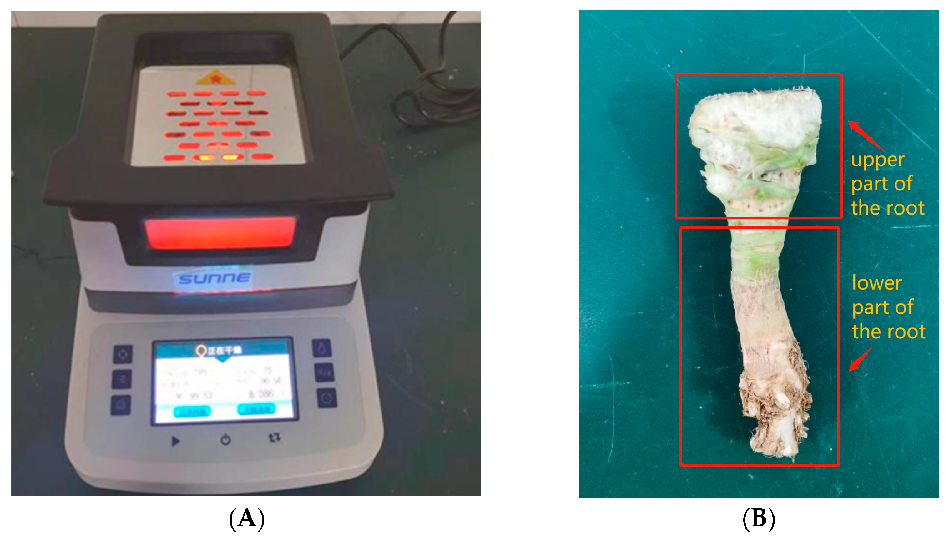
In this experiment, Jingfeng No. 1 kale, developed by the Institute of Vegetable and Flower Research of the Chinese Academy of Agricultural Sciences, was planted in Changsha Wangcheng District, Hunan Province, with a maturity period of 85–90 days. The kale was planted in July and matured in November. The average moisture content in the root stubble of Jingfeng No. 1 kale was measured as 75.94% using an SN-DHS-20A moisture meter, as shown in Figure 2A. The total root length was measured to be 9–16 cm, the diameter of the upper part of the rhizome was 3.9–5.1 cm, and the diameter of the lower part of the rhizome was 1.6–2.5 cm, with an average density of 1.106 g/cm³, as shown in Figure 2B. The kale was planted in a monopoly [15], and the checkerboard sampling method was used to ensure the accuracy of the test. The shear blade material was 45 steel, 2 mm thick, with a 30-degree blade opening angle. A CMT6104 electronic universal test bench was used for the kale root stubble mechanical shear test.

2.1.3. Shear Test Results and Analysis

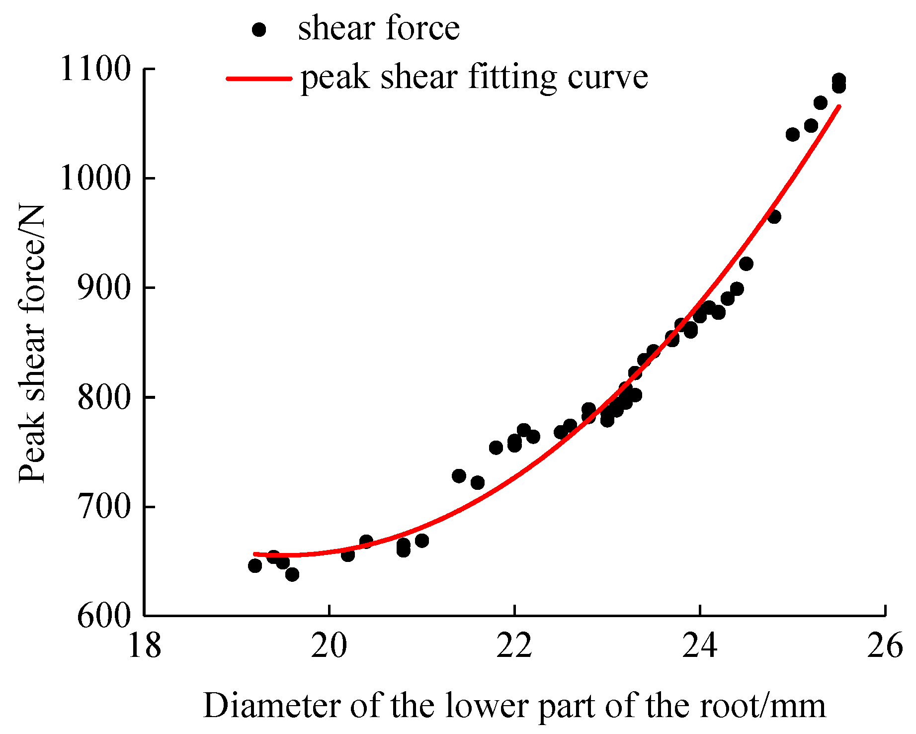
The test results showed that at the lower end of the kale root stubble diameter (19.2–25.5 mm), the shear force was 646–1084 N. The peak shear force of the root increased with an increase in the root diameter. In this test, the shear force was largest for a 25.5 mm root stubble diameter, with a value of 1084 N, and smallest for a 19.2 mm root stubble diameter, with a value of 646 N. As shown in Figure 3, the root stubble end diameter was quadratically related to the peak shear force in Equation (1), with a correlation coefficient of R² = 97.27 and an adjusted R² = 97.154:

$$y=11.4041x^2-444.8293x+4993.3141$$

(1)

2.2. Data Processing Methods

• Single-Factor Test

In the single-factor test design, there is only one study factor used in the experiment, i.e., the researcher analyzes only the effect of one factor on the effect indicator. However, a single-factor test design does not mean that only one factor in that experiment is associated with the effect indicator. One of the main objectives of a single-factor test design is to control the influence of non-study factors on the results of the study [16]. In this paper, seven factors, root stubble modulus of elasticity, bond radius coefficient of simulated particles, contact radius, compressive strength, shear strength, normal stiffness per unit area, and tangential stiffness per unit area were screened out for one-way analysis, and the range of values for each factor was derived from the one-way analysis.

• Plackett–Burman Test

Based on a single-factor test, the Plackett–Burman test can be used when there are many test factors to screen out factors that have a significant effect on the test results [17,18].

• Steepest Climb Test

Based on the results of the Plackett–Burman test, the steepest climb test was conducted on the factors with significance so that the level of the test factors quickly approached the optimal range.

• Box–Behnken Test

Based on the results of the steepest climb test trials, a response surface test was conducted with critical tangential stiffness, critical normal stiffness, and contact radius as independent variables and relative error as the response value. A total of 17 response surface tests with 3 factors and 3 levels were designed to investigate the effects of the variables on the response values.

3. Model Building and Parameter Selection

3.1. Hertz–Mindlin with Bonding V2 Contact Model

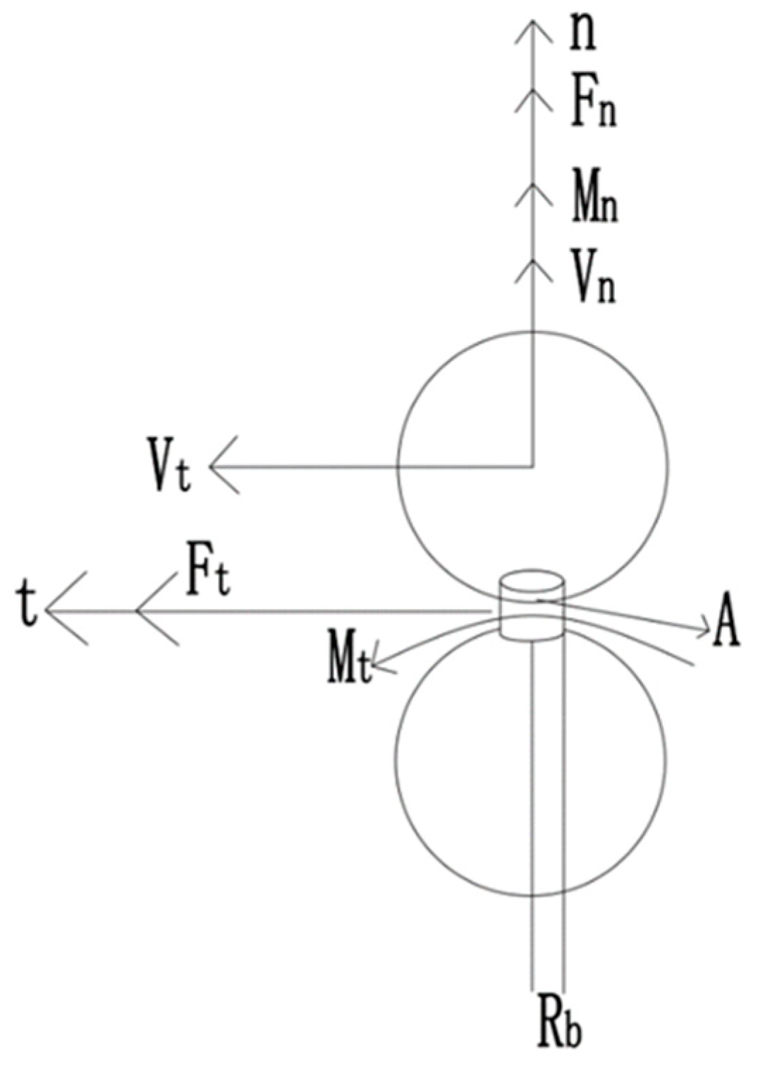
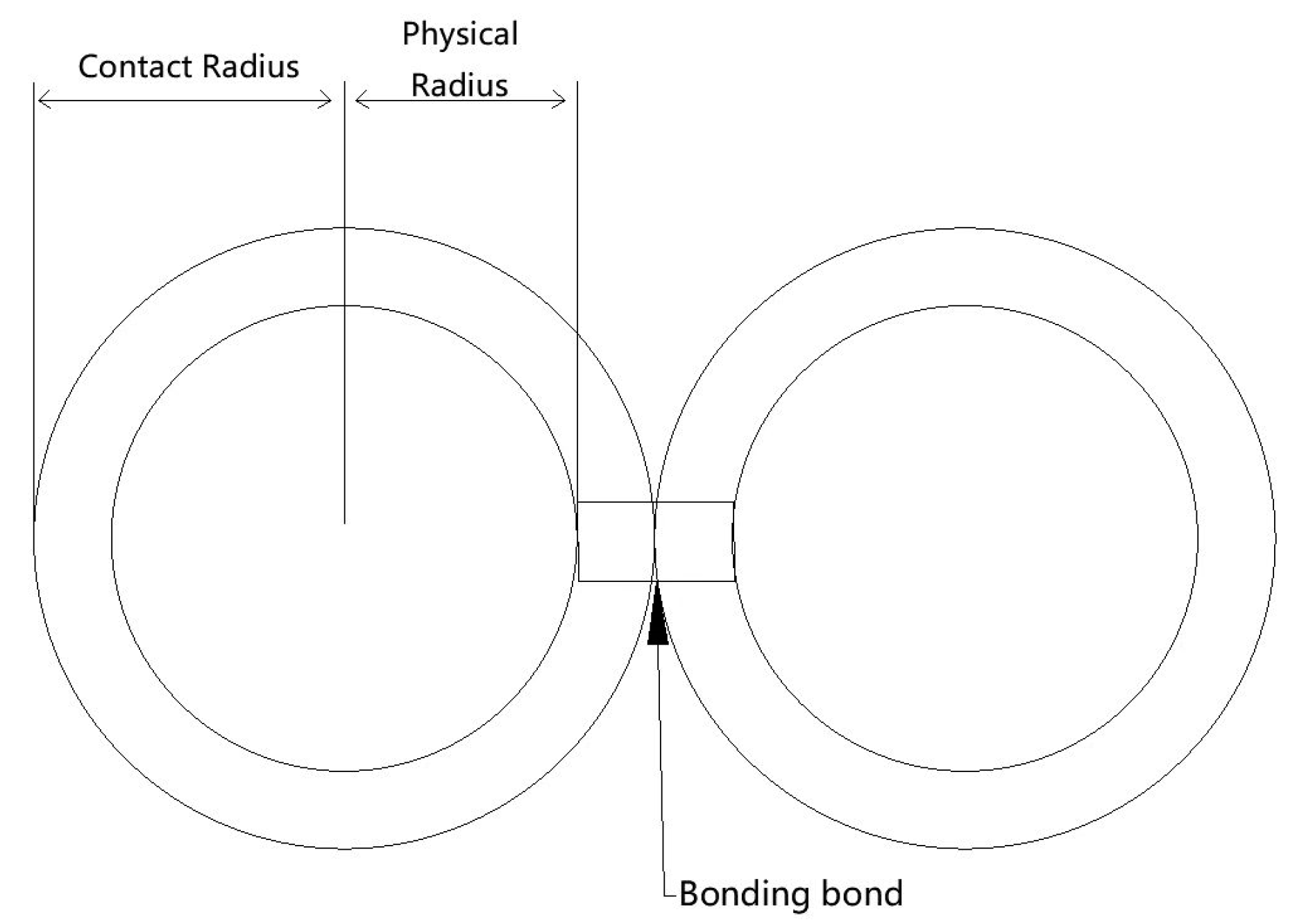
The discrete unit method is widely used in our industry [19,20,21,22,23], agriculture [24,25,26], and construction [27] as a reliable test method and tool [28]. In 1971, CUNDALL proposed a numerical simulation method to solve discontinuous media problems, the discrete element method (DEM), based on the theory of combining different instantons [29]. This paper is based on EDEM2021.2 discrete element software for simulation. The existing discrete element software, in principle, has no big difference compared with other discrete element software using the command operation mode. Whether it is pre-processing modeling or post-processing, a variety of data charts are very convenient to extract from EDEM discrete element software; at the same time, EDEM is able to use the spherical filling method for a variety of non-spherical particle modelings, and in the computational process. The computational efficiency of the software is also better than many other discrete element software; EDEM also supports the implementation of coupling with a variety of software, such as ADAMS and CFD, to deal with a variety of complex situations. In EDEM discrete element software, the contact and bonding principles of the Hertz–Mindlin with bonding V2 contact model and the Hertz–Mindlin with bonding contact model are essentially the same, as shown in Figure 4 and Figure 5, where n and t represent the normal direction and tangential direction, respectively. The main difference is that the bonding V2 model is based on a bonding model with a meta-particle function and a particle coordinate import function, which is more suitable for generating multiple or single irregular models composed of multiple particles at one time. The meta-particle function of this model was used to build a model of oil tea fruit shells. The compressive load–displacement curve in the simulation test was largely consistent with the physical experimental results, which verified the accuracy of the DEM model for oil tea fruit [30]. The Hertz–Mindlin with bonding V2 contact model, as an important model in discrete element simulation, has been widely used in simulation tests for various crops such as forage [31] and castor [32]. This model establishes a finite bond between two particles and performs a combined arrangement or stacking of multiple particles to simulate the target. The bond between the two particles is subjected to forces in the tangential and normal directions. The particles have flexible characteristics in the limited force range and fracture after being subjected to maximum shear and maximum normal forces. Thereafter, the particles interact in the form of hard spheres. After the bond is created, the bond force and moment are set to zero, and the superimposed increments of the bond force and moment applied at each time step can be found. The expressions are as follows (2)–(9):

$$\delta F_n=-v_n{S}_{n}A{\delta }_t$$

(2)

$$\delta F_t=-v_t{S}_{t}A{\delta }_t$$

(3)

$$\delta M_n=-{\omega }_n{S}_{t}J{\delta }_t$$

(4)

$$\delta M_t=-{\omega }_t{S}_n\frac{J}{2}{\delta }_t$$

(5)

$$A=\pi R_B^2$$

(6)

$$J=\frac{1}{2}\pi R_B^4$$

(7)

where $F_n$ is the normal force on the bond of the particle, $F_t$ is the tangential force on the particle bond, $M_n$ is the normal moment of the particle bond, $M_t$ is the tangential moment of the particle bond$, V_n$ is the normal velocity of the particle, $V_t$ is the tangential velocity of the particle$, S_n$ is the normal stiffness of the bond, $S_t$ is the bond tangential stiffness, ${\omega }_n$ is the particle normal angular velocity, ${\omega }_t$ is the particle tangential angular velocity, $A$ is the contact area, $J$ is the bonded spherical spatial moment of inertia, $R_B$ is the bond radius, and ${\delta }_t$ is the time step.

The bond breaks when the tangential and normal stresses on the bond between the particles reach their limits, as expressed by the following Equations (8) and (9):

$${\tau }_{\max }<\frac{-F_t}{A}+\frac{M_n}{J}{R}_B$$

(8)

$${\sigma }_{\max }<\frac{-F_n}{A}+\frac{2M_t}{J}{R}_B$$

(9)

3.2. Selection of Physical Parameters for Kale Root Stubble

After measurement, the kale root density was 1165 kg/m³. According to the literature, Poisson’s ratio of plant roots, root-to-steel and root-to-root recovery coefficients, the static friction factor, and the rolling friction factor have a small effect on the peak shear size, so the relevant surface parameters of maize straw were referenced. The recovery coefficient between roots was set to 0.485, the static friction factor between roots was set to 0.142, the dynamic friction factor between roots was set to 0.078, the recovery coefficient between the root and tool jig was set to 0.663, the static friction factor between the root and tool jig was set to 0.226, and the dynamic friction factor between the root and tool jig was set to 0.119 [33]. The tool material used for the tests was 45 steel with Poisson’s ratio of 0.3, a density of 7820 kg/m³, and a shear modulus of 8 × 10¹⁰ Pa, as shown in

Table 1. Stubble particles and geometric model simulation parameters.

Parameters	Value
Coefficient of restitution between Cabbage stubble	0.485
Coefficient of static friction between Cabbage stubble	0.142
Coefficient of rolling friction between Cabbage stubble	0.078
Coefficient of restitution between Cabbage stubble and steel	0.663
Coefficient of static friction between Cabbage stubble and steel	0.226
Coefficient of rolling friction between Cabbage stubble and steel	0.119
Poisson’s ratio of steel	0.3
Density of steel/(kg/m3)	7800
Shear modulus of steel/(Pa)	8 × 1010

.

3.3. Kale Root Stubble Model

Kale root stubble was selected from the Jingfeng No. 1 variety; the diameter of the lower end of the kale root stubble sampled in the experiment ranged from 19.2 mm to 25.5 mm, and the peak shear force ranged from 646 N to 1084 N. The experimental results showed that 52% of the diameter of the kale root stubble of the Jingfeng No. 1 variety was 23 mm to 25 mm. The experiment was conducted on the lower end of the kale root stubble with a diameter of 24 mm and length of 93 mm to model the lower end of kale. In this experiment, the lower end of the kale root crop with a diameter of 24 mm and length of 93 mm was used to establish the model.

The kale root crop consists of an outer epidermis and inner flesh, and the corresponding model should be anisotropic. The model of the lower end of the kale stubble established in this study is mainly used in the process of using a knife to break the kale roots, and most of its working mode is transverse cutting. Thus, in actual modeling, the model of the lower end of the kale stubble is simplified and set as an isotropic material. The discrete cell method was used to create the root stubble model, and a bonding force was generated between each particle, which was used to fill the fixed frame with particles and generate a bond to form the lower end of the kale root stubble model shown in Figure 6 and Figure 7. The bonding model was chosen to be the bonding V2 model. A cylindrical geometry with a diameter of 24 mm and a length of 100 mm was established, and the cylindrical geometry was filled with the particles. The radius of the particles was set to 1 mm, and the filling coefficient of the particles was set to 0.6. The particle radius was set to 1 mm, and the particle filling factor was 0.6. The position of the generated particles was exported, and meta-practice was employed to import the coordinates to generate a root model with a diameter of 24.02 mm and a length of 92.99 mm. All data processing in this paper was performed using Design-Expert 13 software; the simulation software was EDEM2021.2, and the drawing software was Solidworks2020.

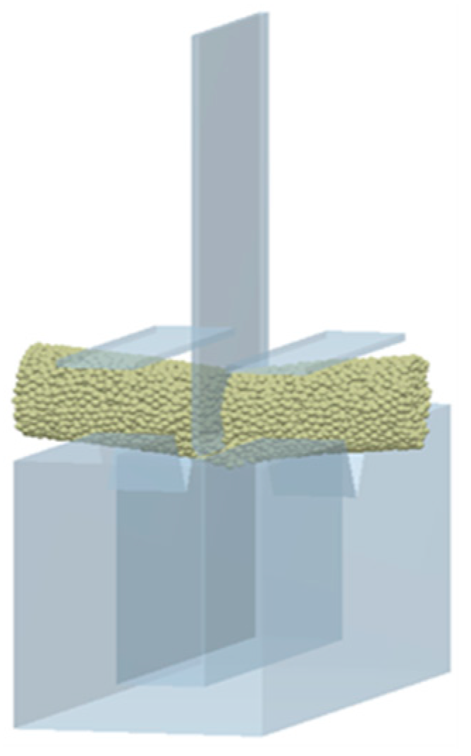
Using the SOLIDWORKS2020 software, the blade and fixture model was saved as an IGS file and imported into the EDEM2021.2 software. The root stubble model with bonding force was also imported (Figure 8), setting the simulation duration to 10 s, the tool travel speed to 5 mm/s, the time step to 15%, and the saving interval to 0.05 s. According to Newton’s third law, the force exerted by the tool instantaneously cutting downwards through the kale root stubble is equivalent to the shear force exerted on the kale root stubble. Thus, the peak force exerted on the tool according to the root stubble is the critical shear force exerted on the kale root stubble. This test uses the relative error between the critical shear force of the actual tool cutting the kale root and the maximum load to which the tool is subjected in the simulation by the kale root stubble as the evaluation index. The equation is as follows:

$$P=\frac{F-F_f}{F}$$

(10)

4. Analysis and Discussion of Results

4.1. Single-Factor Test and Analysis of Results

4.1.1. Single-Factor Test

Using the relative error between the critical shear force of the tool cutting kale roots in the simulation and the actual test and maximum load on the tool by the kale root model in the simulation as the evaluation index, a single-factor experiment was conducted considering seven factors: the modulus of elasticity of the root stubble, the bond radius coefficient of the simulated particles, the contact radius, the compressive strength, the shear strength, the normal stiffness per unit area, and the tangential stiffness per unit area. These factors were used to analyze the product of the bond radius factor, and the radius of the smallest particle is the actual radius of the bond. The contact radius is the radius at which contact between the smallest particles occurs, and the compressive strength is the strength of the bond against tensile forces along the long axis. The shear strength is the strength of the bond against shear forces along the orthogonal plane of the main axis, the normal stiffness per unit area is the tensile and compressive stiffness along the long axis of the bond, and the shear stiffness per unit area is the shear stiffness in the orthogonal plane of the main axis of the bonded bond. In addition, kale root lignification is high. Here, the modulus of elasticity refers to the mechanical design manual in cross-grained wood under 0.5–0.98 GPa. We set the serial number of each factor and the range of values as shown in

Table 2. Corresponding values for each factor in the one-way analysis of variance.

Sign	Parameters	A	B	C	D
X1	Elastic modulus/Pa	1 × 107	5 × 107	1 × 108	5 × 108
X2	Bonded disk scale	1	1.25	1.5	1.75
X3	Normal stiffness per unit area/N/m3	106	107	108	109
X4	Shear stiffness per unit area/N/m3	106	107	108	109
X5	Normal strength/Pa	106	107	108	109
X6	Shear strength/Pa	106	107	108	109
X7	Contact radius/mm	1.5	2	2.5	3

Annotations: A, first level; B, second level; C, third level; D, fourth level.

, in which the fixed parameters are a modulus of elasticity of 5 × 10⁸ Pa, bond radius coefficient of 1.5, contact radius of 2.5, compressive strength of 1 × 10⁸ Pa, shear strength of 1 × 10⁸ Pa, normal stiffness per unit area of 1 × 10⁸ N/m³, and tangential stiffness per unit area 1 × 10⁸ N/m³.

4.1.2. Analysis of the Results of the Single-Factor Test

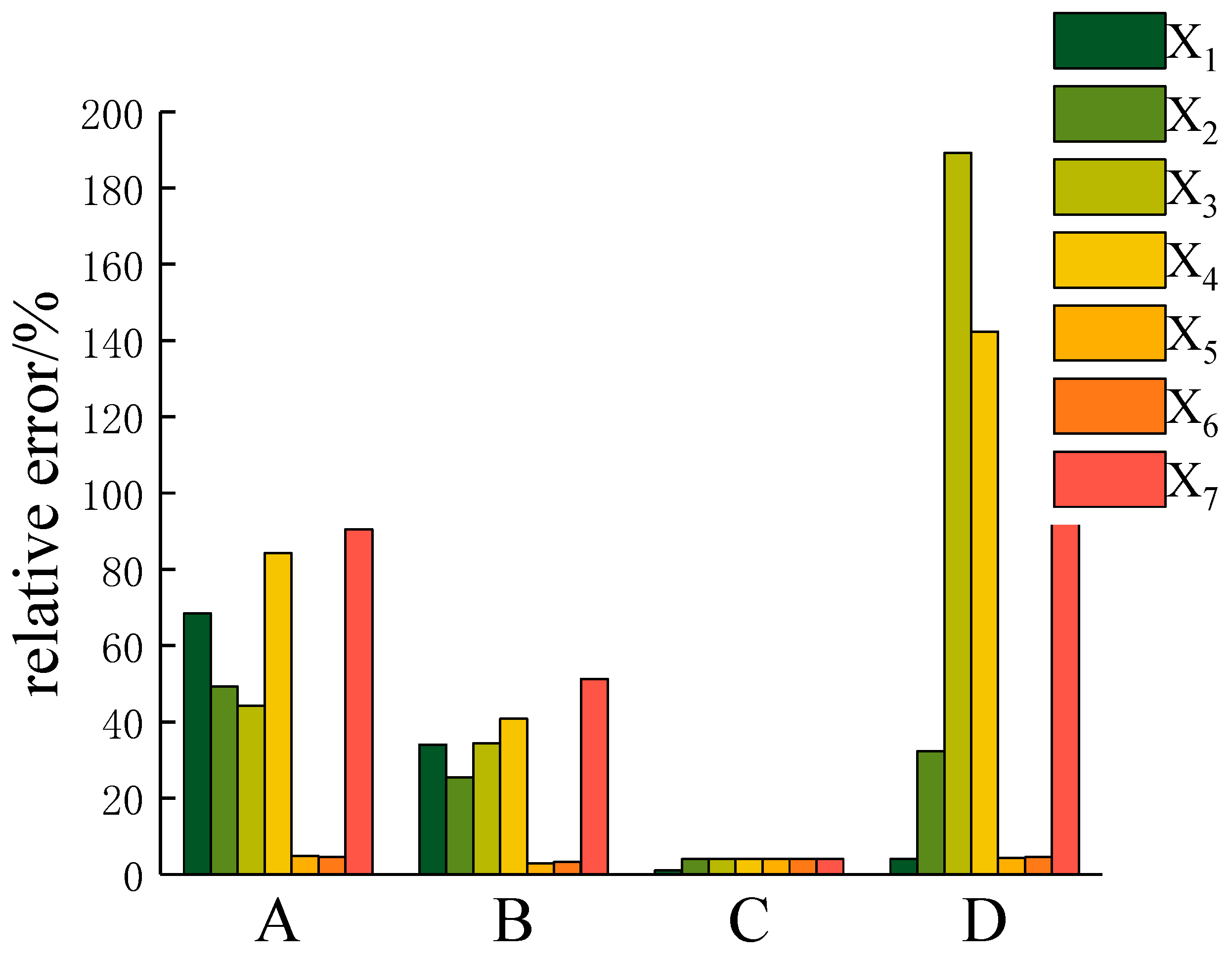
As shown in Figure 9, according to the results of the one-way test, the relative error is larger when the modulus of elasticity is 1 × 10⁷ Pa and 5 × 10⁷ Pa, and the difference in the relative error is smaller when the modulus of elasticity is 1 × 10⁸ Pa and 5 × 10⁸ Pa. The smallest relative error was found when the modulus of elasticity was 1 × 10⁸ Pa. The relative error according to the bond radius coefficient tends to increase and then decrease; when the bond radius coefficient is 1.5, the relative error is the smallest. When the unit area normal stiffness increases, the relative error shows a trend of rapidly decreasing and then increasing, where the relative error is smaller when the critical tangential stress is 1 × 10⁸ Pa, and the relative error is larger in the remaining cases. The relative error trend shows a tendency to decrease first and then increase rapidly when the tangential stiffness per unit area increases. When the critical normal stress is 1 × 10⁸ Pa, the relative error is the smallest, and when the critical normal stress is 1 × 10⁹ Pa, the relative error is the largest. When the compressive strength and shear strength increase, the magnitude of the relative error change is not obvious. Changes in the particle contact radius tend to first decrease and then increase the relative error. In addition, the number of discrete element particles increases as the radius increases, and the number of bonding bonds between particles increases, resulting in an increase in both the shear force and relative error. As the particle radius decreases, the bonding bonds between particles are reduced, resulting in a decrease in the shear force and an increase in the relative error. The relative error is minimized when the contact radius of the particles is 2.5 mm. By analyzing the results of the single-factor test, we determined the general range of the value of each factor, as well as its high and low levels, as shown in

Table 3. Plackett–Burman test model parameters.

Sign	Parameters	High Level	Low Level
X1	Elastic modulus/Pa	1 × 108	5 × 107
X2	Bonded disk scale	1.5	1.25
X3	Normal stiffness per unit area/N/m3	1 × 108	1 × 107
X4	Shear stiffness per unit area/N/m3	1 × 108	1 × 107
X5	Normal strength/Pa	1 × 108	1 × 107
X6	Shear strength/Pa	1 × 108	1 × 107
X7	Contact radius/mm	2.5	2

.

4.2. Plackett–Burman Test and Analysis of Results

4.2.1. Plackett–Burman Test

In this study, the elastic modulus of root stubble, the bond radius coefficient of the simulated particles, the contact radius, the critical normal stress, the critical tangential stress, the normal contact stiffness, and the tangential contact stiffness were selected based on the two levels of the Plackett–Burman test using the Design Expert software. The number of tests was set to 12 for the Plackett–Burman test, as shown in

Table 4. Plackett–Burman test results.

No.	X1/(Pa)	X2	X3/(N/m3)	X4/(N/m3)	X5/(Pa)	X6/(Pa)	X7/(mm)	Relative Error/(%)
1	5 × 107	1.25	1 × 108	1 × 107	1 × 108	1 × 108	2	87.36
2	5 × 107	1.5	1 × 107	1 × 108	1 × 108	1 × 107	2.5	61.28
3	1 × 108	1.25	1 × 107	1 × 107	1 × 108	1 × 107	2.5	91.82
4	5 × 107	1.5	1 × 108	1 × 107	1 × 108	1 × 108	2.5	41.67
5	1 × 108	1.25	1 × 108	1 × 108	1 × 108	1 × 107	2	70.44
6	1 × 108	1.5	1 × 107	1 × 108	1 × 108	1 × 108	2	74.98
7	1 × 108	1.25	1 × 108	1 × 108	1 × 107	1 × 108	2.5	5.37
8	5 × 107	1.5	1 × 108	1 × 108	1 × 107	1 × 107	2	59.7
9	5 × 107	1.25	1 × 107	1 × 108	1 × 107	1 × 108	2.5	61.28
10	5 × 107	1.25	1 × 107	1 × 107	1 × 107	1 × 107	2	97.31
11	1 × 108	1.5	1 × 108	1 × 107	1 × 107	1 × 107	2.5	42.22
12	1 × 108	1.5	1 × 107	1 × 107	1 × 107	1 × 108	2	95.98

.

4.2.2. Analysis of Plackett–Burman Test Results

As shown in

Table 5. Plackett–Burman test ANOVA.

Sign	Effect	Mean Square	Impact	p-Value	Significance Ranking
X1	−2.32	64.36	0.4257	0.5497	7
X2	−3.15	118.76	0.7855	0.4255	6
X3	−14.66	2578.11	17.05	0.0145	2
X4	−10.28	1267.11	8.38	0.0443	3
X5	5.47	359.6	2.38	0.1979	4
X6	−4.68	262.55	1.74	0.258	5
X7	−15.18	2764.28	18.28	0.0129	1

, the results of the Plackett–Burman test showed that among the seven factors (i.e., the modulus of elasticity, bond radius coefficient of the simulated particles, contact radius, critical normal stress, critical tangential stress, normal contact stiffness, and tangential contact stiffness), the p-values for the critical normal stress, critical tangential stress, and contact radius were <0.05, indicating that these three factors had a significant effect on the relative error. The p-values for the radius, normal contact stiffness, and tangential contact stiffness were >0.05, indicating that the effect on the relative error was not significant. Therefore, the critical normal stress, critical tangential stress, and contact radius were selected for the steepest climb test and the Box–Behnken test to quickly approximate the optimum range and investigate the effect of the test factors and their interaction terms on the relative error. Here, the four factors without significant effects on the relative error, i.e., the modulus of elasticity, radius coefficient, normal contact stiffness, and tangential contact stiffness, are taken to be 1 × 10⁸ Pa, 1.5, 1 × 10⁷ N/m³, and 1 × 10⁷ N/m³, respectively.

4.3. Steepest Climb Test and Analysis of Results

4.3.1. Steepest Climb Test

To more quickly bring the most significant factors in the Plackett–Burman test closer to the optimal range of values, the steepest climbing test was carried out for the significant factors based on the results of the Plackett–Burman test. This test was carried out using six trials, resulting in an average peak shear force closer to the mechanical test.

4.3.2. Analysis of the Results of the Steepest Climb Test

Based on the results of the steepest climb test shown in

Table 6. Steepest climb test results.

Test Number	X3/107 (N/m3)	X4/107 (N/m3)	X7/(mm)	Peak Shear Force/N	Relative Error/(%)
1	1	1	2	34.4	95.98
2	2	2	2.1	96.4	88.74
3	4	4	2.2	194.7	77.25
4	6	6	2.3	382.4	55.32
5	8	8	2.4	527.1	38.41
6	10	10	2.5	864.5	1.02

, when the critical tangential stiffness is 1 × 10⁸ N/m³, the critical normal stiffness is 1 × 10⁸ N/m³, and the contact radius is 2.5 mm. Additionally, the error in relation to the mean peak shear in the shear test is the smallest, at 1.02%. Therefore, the non-significant factor radius factor, normal contact stiffness, and tangential contact stiffness were taken to be 1.5, 1 × 10⁷ N/m³, and 1 × 10⁷ N/m³, respectively. We used a critical tangential stiffness of 1 × 10⁸ N/m³, a critical normal stiffness of 1 × 10⁸ N/m³, and a contact radius of 2.5 mm as the intermediate level; a critical tangential stiffness of 1.02 × 10⁸ N/m³, a critical normal stiffness 1.02 × 10⁸ N/m³, and a contact radius of 2.52 mm as the high level; and a critical tangential stiffness of 9.8 × 10⁷ N/m³, a critical normal stiffness of 9.8 × 10⁷ N/m³, and a contact radius of 2.48 mm as the low level for the Box–Behnken test.

4.4. Box–Behnken Test and Analysis of Results

4.4.1. Box–Behnken Test

Based on the results of the steepest climb test, a Box–Behnken test design was carried out with critical tangential stiffness, critical normal stiffness, and contact radius as independent variables and the relative error as the response value to derive the relationship between the critical tangential stiffness, critical normal stiffness, contact radius, and their interaction terms and relative errors. The test results are shown in

Table 7. Box–Behnken test results.

Test Number	X3/107 (N/m3)	X4/107 (N/m3)	X7/(mm)	Relative Error/(%)
1	9.8 × 107	1 × 108	2.48	5.68
2	1 × 108	1 × 108	2.5	1.86
3	1.02 × 108	1 × 108	2.52	14.85
4	1 × 108	1 × 108	2.5	1.11
5	1.02 × 108	1 × 108	2.5	1.11
6	1 × 108	1.02 × 108	2.48	2.8
7	1 × 108	1.02 × 108	2.5	1.86
8	1 × 108	9.8 × 107	2.52	10.8
9	1 × 108	9.8 × 107	2.48	0.65
10	1 × 108	1 × 108	2.5	1.11
11	9.8 × 107	9.8 × 107	2.5	5.03
12	1.02 × 108	1.02 × 108	2.5	11.2
13	1.02 × 108	1 × 108	2.48	5.26
14	9.8 × 107	1 × 108	2.52	7.58
15	9.8 × 107	1.02 × 108	2.5	5.2
16	1.02 × 108	9.8 × 107	2.5	6.68
17	1.02 × 108	1.02 × 108	2.52	11.37

.

4.4.2. Box–Behnken Test Results and Analysis

The Box–Behnken regression model ANOVA (

Table 8. Analysis of variance for Box–Behnken regression models.

Source	Sum of Squares	df	Mean Square	F-Value	p-Value
Model	268.97	9	29.89	46.49	<0.0001
X3	19.75	1	19.75	30.72	0.0009
X4	4.53	1	4.53	7.05	0.0327
X7	115.9	1	115.9	180.29	<0.0001
X3×4	2.45	1	2.45	3.81	0.0919
X3×7	26.52	1	26.52	41.26	0.0004
X4×7	1.6	1	1.6	2.49	0.1586
X32	48.22	1	48.22	75	<0.0001
X42	9.88	1	9.88	15.36	0.0058
X72	30.9	1	30.9	48.07	0.0002
Residual	4.5	7	0.6429
Lack of Fit	2.05	3	0.682	1.11	0.4426
Pure Error	2.45	4	0.6135
Cor Total	273.47	16

) shows that the model coefficient of determination R = 98.35, indicating a high model fit, and the model p-value < 0.001, indicating that the regression equation is highly significant. In the regression model, the primary terms X₃ and X₇ are highly significant; the interaction term X_3×7, with a p-value < 0.001, indicates that this interaction term has a highly significant effect on the regression model; the interaction terms X_3×4 and X_4×7 are not significant; the secondary terms X₃², X₄², and X₇² are highly significant; and the misfit term has a p-value > 0.05, indicating that there are no other significant factors affecting the response values in this model.

When the unit area normal stiffness value is fixed, the relative error does not change significantly as the unit area tangential stiffness increases. When the unit area tangential stiffness value is fixed, the relative error tends to increase as the unit area normal stiffness increases. The unit area normal stiffness has a higher effect on the relative error than the unit area tangential stiffness, and the interaction term between the unit area normal stiffness and the unit surface tangential stiffness is not significant (Figure 10a).

When the unit area tangential stiffness value is constant, the relative error increases with an increase in the contact radius and changes more significantly. When the contact radius is constant within a certain range, the fluctuation of the relative error with the unit area tangential stiffness value is not significant, and the unit area tangential stiffness and contact radius interaction term are also not significant (Figure 10b).

The influence of the interaction term between the contact radius and unit area normal stiffness on the relative error is more obvious. When the value of the unit area normal stiffness is constant, the relative error tends to increase as the contact radius increases; when the contact radius is fixed, the relative error tends to decrease and then increases as the unit area normal stiffness increases (Figure 10c).

4.4.3. Optimal Model Validation

To obtain the simulated average peak force and its parameter combinations that are closest to the average peak shear in the actual shear test, the regression model was optimized using the Design-Expert software, and the optimal parameter combinations were obtained as follows: normal stiffness per unit area of 9.965 × 10⁷ N/m³, tangential stiffness per unit area of 9.949 × 10⁷ N/m³, and contact radius of 2.4818 mm. A theoretical relative error of 0.63% was predicted. Simulation tests were carried out using the optimized parameters and verified, yielding a simulated average peak shear of 861.02 N, with a relative error of 0.61% compared to the average peak shear of 855.8 N in the actual shear tests. These test results are close to the model predictions, indicating that the model is accurate and reliable.

5. Conclusions

In this study, discrete element modeling and the calibration of kale root stubble were carried out using EDEM2021.2 discrete element simulation software, and the experimental method and content were designed using the Design-Expert software. Based on a shear test and data measurements using a certain sample size of kale root stubble, a one-factor analysis, Plackett–Burman test, steepest climb test, and Box–Behnken test were carried out. The factors affecting the relative error were subjected to range taking, significance analysis, target value approximation, response surface analysis, etc. Finally, model optimization and validation were carried out.

The tendency of the relative error to fluctuate with a change in the size of each factor was determined through a one-factor test, and the range of values for each factor was determined as follows: modulus of elasticity, 1 × 10⁸–5 × 10⁸ Pa; radius coefficient, 1.25–1.5; normal stiffness per unit area, 5 × 10⁷–1 × 10⁸ N/m³; and tangential stiffness per unit area, 5 × 10⁷–1 × 10⁸ N/m³. The compressive strength was 1 × 10⁷–1 × 10⁸ Pa, the shear strength was 1 × 10⁷–1 × 10⁸ Pa, and the contact radius was 2–2.5 mm.

The Plackett–Burman test was used to screen out the three factors with a significant influence on the relative error, which were the normal stiffness per unit area, tangential stiffness per unit area, and contact radius. We selected the high and low extremes close to the real values in the range as the high and low levels for the steepest climb test using the corresponding parameter simulation results. The relative error was only 1.02%.

The relative error response characteristics between the three significant factors and the target calibration value were obtained via the Box–Behnken test. At the same time, we found that the normal stiffness per unit area had a more obvious interaction with the contact radius. The regression model was optimized using the Design-Expert software, and the optimized parameters were obtained as follows: the normal stiffness per unit area was 9.965 × 10⁷ N/m³, the tangential stiffness per unit area was 9.949 × 10⁷ N/m³, and the contact radius was 2.4818 mm. The final data were imported into EDEM2021.2 simulation software for validation simulation tests, and the peak shear of the validation tests was 861.02 N, which had a relative error of 0.61% from the real measured average peak shear. The analyzed data showed that the simulation parameters of the discrete element model of kale root stubble had good reliability and accuracy.

References

1. Zeng, A.; Xia, P.; Yan, J.; Xu, Y.; Xing, M.; Lu, Y. Analysis on Market Demand Changes of Cabbage Cultivars in China. J. Chang. Veg. 2022, 8, 1–3. [Google Scholar]
2. Sabine, J.; Jutta, L. Response of Arabidopsis thaliana Roots with Altered Lipid Transfer Protein (LTP) Gene Expression to the Clubroot Disease and Salt Stress. Plants 2015, 5, 2. [Google Scholar]
3. Zhao, J.; Song, W.; Li, J. Modeling and Mechanical Properties Analysis of Rice Straw Based on EDEM. Chin. J. Soil Sci. 2020, 51, 1086–1093. [Google Scholar]
4. Kenny, D.N.; Bart, L.; Erdal, K.; Wouter, S. Bulk compression characteristics of straw and hay. Biosyst. Eng. 2014, 118, 194–202. [Google Scholar]
5. Adajar, J.B.; Alfaro, M.; Chen, Y.; Zeng, Z. Calibration of discrete element parameters of crop residues and their interfaces with soil. Comput. Electron. Agric. 2021, 188, 106349. [Google Scholar] [CrossRef]
6. Fang, M.; Yu, Z.; Zhang, W.; Cao, J.; Liu, W. Friction coefficient calibration of corn stalk particle mixtures using Plackett-Burman design and response surface methodology. Powder Technol. 2022, 396, 731–742. [Google Scholar] [CrossRef]
7. Tong, S.; Shao, M.; Cao, M.; Zhao, J. Parameter Calibration of Corn Straw Discrete Element Model Based on DEM. J. Chin. Agric. Mech. 2023, 44, 69–75. [Google Scholar]
8. Schramm, M.; Tekeste, M.Z. Wheat straw direct shear simulation using discrete element method of fibrous bonded model. Biosyst. Eng. 2022, 213, 1–12. [Google Scholar] [CrossRef]
9. Hou, J.; Xie, F.; Wang, X.; Liu, D.; Chen, Z. Measurement of Contact Physical Parameters of Flexible Rice Straw and Discrete Element Simulation Calibration. Acta Agric. Univ. Jiangxiensis 2022, 44, 747–758. [Google Scholar]
10. Zhang, Y.; Ren, D.; Gong, Y.; Li, J.; Cheng, H.; Zhang, L. Calibration of contact parameters of straw biochar based on discrete element method. Acta Energiae Solaris Sin. 2022, 43, 345–351. [Google Scholar]
11. Mirko, M.; Luisa, M.; Nicolò, R.; Giovanni, M. Analysis of the parameters affecting the mechanical behaviour of straw bales under compression. Biosyst. Eng. 2017, 160, 179–193. [Google Scholar]
12. Liu, W.; Su, Q.; Fang, M.; Zhang, J.; Zhang, W.; Yu, Z. Parameters Calibration of Discrete Element Model for Corn Straw Cutting Based on Hertz-Mindlin with Bonding. Appl. Sci. 2023, 13, 1156. [Google Scholar] [CrossRef]
13. Liu, D.; Liu, Z.; Wang, Q.; Li, X.; Yan, C. Calibration of contact parameters for bamboo powder particles based on DEM. J. Zhejiang AF Univ. 2023, 40, 875–882. [Google Scholar]
14. Zhang, T.; Liu, F.; Zhao, M.; Ma, Q.; Wang, W.; Fan, Q.; Yan, P. Determination of corn stalk contact parameters and calibration of Discrete Element Method simulation. J. China Agric. Univ. 2018, 23, 120–127. [Google Scholar]
15. Wang, X. Cultivation techniques for efficient ground cover cultivation of knotted kale. Vegetables 2021, 6, 45–47. [Google Scholar]
16. Duan, A.; Li, X.; Yan, K. Optimization of the Technological Formula of Bamboo Juice Jelly by Response Surface Methodology Based on Single Factor Experiment. China Food Saf. Mag. 2022, 8, 152–155. [Google Scholar]
17. Bhupendra, M.G.; Manish, P.; Rohit, N.; Gopal, C. Calibration of discrete element model parameters: Soybeans. Comput. Part. Mech. 2019, 6, 3–10. [Google Scholar]
18. Bart, L.; Thomas, A.; Engelbert, T.; Bart, D.K.; Herman, R.; Josse, D.B.; Wouter, S. Simulation of grain–straw separation by Discrete Element Modeling with bendable straw particles. Comput. Electron. Agric. 2014, 101, 24–33. [Google Scholar]
19. Liu, Y.; Gao, D.; Li, X.; Qin, X.; Li, H.; Liu, H. Investigating the Jet Comminuting Process in Cuttings Transport by Coupling the CFD/DEM Method and Bonded-Particle Model. SPE J. 2019, 24, 2020–2032. [Google Scholar] [CrossRef]
20. Li, J.P.; Rao, Q.H.; Huang, T.B.; Ma, W.B. Discrete element method for adhesion properties evaluation of deep-sea sediment from macro and micro perspectives. J. Cent. South Univ. 2022, 29, 1701–1716. [Google Scholar] [CrossRef]
21. Shi, Y.; Liu, J.; Huang, D.; Xu, M.; Zhai, S.; Zhang, W.; Jiang, P. Prediction and Experimental Study of Tire Slip Rate Based on Chassis Sinkage Amount. Agriculture 2023, 13, 665. [Google Scholar] [CrossRef]
22. Zhai, S.; Shi, Y.; Zhou, J.; Liu, J.; Huang, D.; Zou, A.; Jiang, P. Simulation Optimization and Experimental Study of the Working Performance of a Vertical Rotary Tiller Based on the Discrete Element Method. Actuators 2022, 11, 342. [Google Scholar] [CrossRef]
23. Kukreja, K.; Soni, M.K.; Nainegali, M.S.; Mohapatra, B. Development of transfer chute design through Discrete Element Modelling for using Refused Derived fuel in Indian cement plants. Sustain. Energy Technol. Assess. 2022, 53, 102567. [Google Scholar] [CrossRef]
24. Chen, J.; Zhou, H.; Che, H.; Liu, Y.; Li, P. Optimal Design of Ejector Belt Seedling Collecting Mechanism Based on EDEM. INMATEH Agric. Eng. 2023, 69, 109–120. [Google Scholar] [CrossRef]
25. Zeng, F.; Li, X.; Bai, H.; Cui, J.; Liu, X.; Zhang, Y. Calibration of the Discrete Element Parameters and Experimental Verification of the Oil Sunflower Plug Seedling Pots. INMATEH Agric. Eng. 2022, 68, 629–640. [Google Scholar] [CrossRef]
26. Sen, Z.; Jie, J.; Yuedong, W. A Study on the Physical Properties of Banana Straw Based on the Discrete Element Method. Fluid Dyn. Mater. Process. 2022, 19, 1159–1172. [Google Scholar]
27. An, H.; Liu, H.; Han, H. Hybrid Finite-Discrete Element Modelling of Excavation Damaged Zone Formation Process Induced by Blasts in a Deep Tunnel. Adv. Civ. Eng. 2020, 2020, 7153958. [Google Scholar] [CrossRef]
28. Andrew, P.G.; Peter, W.W. Development and validation of calibration methods for discrete element modelling. Granul. Matter 2011, 13, 127–132. [Google Scholar]
29. Zhuo, J.; Zhao, N. Basic principles, methods and applications of the discrete unit method. Adv. Sci. Technol. Water 1993, 13, 1–11. [Google Scholar]
30. Zhang, H.; Li, X.; Yan, F. Discrete element modelling of Camellia oleifera fresh fruit and its simulation. Coll. Mech. Electron. Eng. Northwest AF Univ. 2022, 12344, 141–147. [Google Scholar]
31. Fan, G.; Wang, Z.; Wang, B.; Wang, J.; Dong, H.; Han, J. Design and Experiment of Rotary Feed Tube Hammer Grinder. Trans. Chin. Soc. Agric. Mach. 2021, 52, 43–53. [Google Scholar]
32. Hou, J.; Ren, Z.; Liu, D.; Ma, Z.; Liu, X.; Wang, W. Parameter Calibration of a Discrete Element Model for Three-Compartment Separation and Fragmentation of Castor Capsules During Harvesting. J. Biosyst. Eng. 2023, 48, 198–214. [Google Scholar] [CrossRef]
33. Zhu, H.; Qian, C.; Bai, L.; Li, H.; Mou, D.; Li, J. Optimization of discrete element model of corn stalk based on Plackett-Burman design and response surface methodology. J. China Agric. Univ. 2021, 26, 221–231. [Google Scholar]
Figure 1. Calibration process of the kale root stubble simulation parameters.
Agronomy 13 02298 g001
Figure 2. (A) SN-DHS-20A moisture meter; (B) kale root stubble of Jingfeng No. 1.
Agronomy 13 02298 g002
Figure 3. Relationship between diameter and peak shear at the lower end of kale roots in Jingfeng No. 1.
Agronomy 13 02298 g003
Figure 4. The Hertz–Mindlin with bonding V2 contact model.
Agronomy 13 02298 g004
Figure 5. Discrete element particle bonding model.
Agronomy 13 02298 g005
Figure 6. Simulation model of kale root stubble particles.
Agronomy 13 02298 g006
Figure 7. Kale root stubble bonding bond model.
Agronomy 13 02298 g007
Figure 8. Shear test simulation model.
Agronomy 13 02298 g008
Figure 9. Effects of factors on relative errors in the simulation tests; See notes to Table 2 for ABCD meanings.
Agronomy 13 02298 g009
Figure 10. Effect of interactions between factors on the relative error.
Agronomy 13 02298 g010