Integration of Remote Sensing and Field Observations in Evaluating DSSAT Model for Estimating Maize and Soybean Growth and Yield in Maryland, USA

Abstract

Crop models are useful for evaluating crop growth and yield at the field and regional scales, but their applications and accuracies are restricted by input data availability and quality. To overcome difficulties inherent to crop modeling, input data can be enhanced by the incorporation of remotely sensed and field observations into crop growth models. This approach has been recognized to be an important way to monitor crop growth conditions and to predict yield at the field and regional scale. In recent years, satellite remote sensing has provided high-temporal and high-spatial-resolution data that allow for generating continuous time series of biophysical parameters such as vegetation indices, leaf area index, and phenology. The objectives of this study were to use remote sensing along with field observations as inputs to the Decision Support System for Agro-Technology (DSSAT) model to estimate soybean and maize growth and yield. The study used phenology and leaf area index (LAI) data derived from Planet Fusion (daily, 3 m) satellite imagery along with field observation data on crop growth stage, LAI and yield collected at the United State Department of Agriculture, Agricultural Research Service, Beltsville Agricultural Research Center (BARC), Beltsville, Maryland. For maize, a total of 17 treatments (site years) were used (ten treatments for model calibration and seven treatments for validation), while for soybean (maturity groups three and four), a total of 18 treatments were used (nine for calibration and nine for validation). The calibrated model was tested against an independent, multi-location and multi-year set of phenology and yield data (2017–2020) from BARC fields. The model accurately simulated maize and soybean days to flowering and maturity and produced reasonable yield estimates for most fields and years. Model run for independent locations and years produced good results for phenology and yields for both maize and soybean, as indicated by index of agreement (d) values ranging from 0.65 to 0.93 and normalized root-mean-squared error values ranging from 1 to 20%, except for soybean maturity group four. Overall, model performances with respect to phenology and grain yield for maize and soybean were good and consistent with other DSSAT evaluation studies. The inclusion of remote sensing along with field observations in crop-growth model inputs can provide an effective approach for assessing crop conditions, even in regions lacking ground data.

1. Introduction

Agriculture is one of the major economic sectors in the United States of America (U.S.), contributing approximately $992 billion in revenue to the U.S. economy annually and about 6% of the gross domestic product (GDP) [1,2]. As an example, during the third quarter of 2016 a surge in crop exports (wheat, corn, and soybean) propelled the economy to the best performance in two years [1,2]. Despite these gains, industry leaders envisage that climate variability and change, especially drought and high temperature, could cause about 50% reduction in crop yields unless scientists can develop methods to adapt cropping systems to this changing climate in the 21st century [3,4,5,6]. A decline of 50% in crop production in the U.S. could cost about $400 billion in income and force hundreds of thousands of farmers to abandon their farming, thereby contributing to unemployment and causing global food insecurity [7,8,9]. In fact, to meet growing food demands, global food production needs to double by 2050 [10,11,12]. Due to the combined prevailing factors of climate change, rapid population growth, and soil degradation, a method that provides the timely monitoring of crop conditions and forecasting of yield within the season and at the field and regional level would be a valuable tool to help ensure food security [9,12,13,14]. Crop models such as the Decision Support System for Agro-Technology (DSSAT) are valuable for capturing the effects of soils, climate, management, and cultivar on crop growth and yields. Even though crop models are useful for running scenarios under different kinds of management and climate conditions, these models require detailed information that is often unavailable or of poor quality [15,16,17,18]. Key model inputs include cultivation dates and on-farm decision factors affecting crop development (e.g., cultivar type, planting date, row and plant spacing, and irrigation). Remote sensing provides means for constraining these unknowns. In particular, key phenological stages can be determined from satellite imagery, including date of emergence, peak growth, and senescence. These remotely sensed growth stages can be related to crop cultivation activities and management factors such as the planting date, vegetation stage, and harvest yield. Biomass development, quantified as leaf area index (LAI), can also be estimated with remote sensing. Evapotranspiration estimation from remote sensing can give us information related to irrigation amounts. This information can be used to constrain, or compensate for, unknowables such as cultivar type, fertilizer application, irrigation, and detailed soil variability. Therefore, coupling remote sensing and crop growth models provides the best option for improving our understanding of the factors that limit crop yield and how to improve yield to meet the food security demands of the world [14,19,20].

To overcome difficulties inherent to crop modeling, input data can be enhanced by the integration of remotely sensed and field observations into crop growth models [14,18,19,21,22]. This approach has been recognized as an important way to monitor crop growth conditions and to predict yield at the field and regional scale [22,23,24,25,26,27,28]. In recent years, satellite remote sensing systems have achieved improvement in temporal and spatial resolution data that support the generation of continuous time series of biophysical parameters such as vegetation indices, LAI, phenology, and other crop state variables at the field and regional scale [29,30,31,32,33,34,35]. Therefore, the integration of remote sensing into crop growth models for crop monitoring and yield prediction has become possible and has been proven to be an effective method for regional yield estimation [22,23,24,27,36,37]. Remote sensing can provide missing information, such as spatial information, required by crop models for improved yield forecasting at a regional level [18]. The integrating or inclusion of remote sensing alongside field observations with crop growth models provides an effective tool for assessing crop growth conditions and yield, especially in data-poor regions or regions lacking ground data [19,20,38,39,40]. Early and recent research has shown that remote sensing can provide an inexpensive source of crop growth information for crop modeling [19,20,38,41,42]. Remote sensing can provide timely, non-destructive, instantaneous, and accurate estimations of the crop parameters required for most crop growth models [18]. Field observations commonly are time-consuming, laborious and expensive and rarely made in most field trials [18,19,38,43]. Therefore, integrating remote sensing information into crop growth models for yield prediction has received a lot of attention recently [18,44,45,46]. Additionally, the inclusion of remote sensing and field observations with crop growth models provides an opportunity for near-real-time or within-season assessment of crop growth conditions and the forecasting of yield [18].

The objectives of this study were to (1) derive LAI and crop growth stages using remote sensing observation, and (2) use remotely sensed data along with field observations to calibrate the DSSAT model for soybean and maize growth and yield in an experimental agricultural area. The calibrated model can be scaled up for regional yield prediction and climate change impact study.

2. Materials and Methods

2.1. Description of the Study and Experimental Area

Our study site was carried out at the United State Department of Agriculture, Agricultural Research Service, Beltsville Agricultural Research Center (BARC), Beltsville, Maryland (Figure 1). This site is a Long-Term Agroecosystem Research (LTAR) network and production research site in Maryland and includes ~2670 hectares of agricultural fields. The sizes of the fields vary from 1 hectare to more than 20 hectares [47]. No-till practices were used for all fields in this study. The major crops grown in these fields are maize, soybean, wheat, barley, rye, and cover crops. The dominant soil types range from sandy loams to loamy sands. Climatological conditions at BARC are characteristic of the coastal physiographic zone of the mid-Atlantic Region. The research center keeps a comprehensive record of all planting operations, such as pre-planting operations, planting dates, cultivar name, planting population and row spacing, irrigation and fertilizer applications, and harvest dates for each field using FarmLogic Systems. In this study, for maize, the cultivar used was a medium season cultivar, whereas for soybean, maturity group three and group four were used. The days to flowering and maturity for maturity group three ranged from 37 to 52 and from 93 to 128 days after planting, respectively. For maturity group 4, the days to flowering and maturity ranged from 43 to 50 and from 106 to 126 days after planting, respectively. There were no clear differences in days to flowering and maturity between the maturity groups. This may have been a result of the differences in fields and years used. For the maize cultivar, plants were no-till seeded between 38 cm and 76 cm rows at a density of between 69,000 and 74,000 plants ha⁻¹ from 25 April to 10 June. Soybean crops were no-till and seeded between 19cm and 76cm rows at a density of between 383,000 and 445,000 plants ha⁻¹ from 20 April to 28 June. Both cultivars were grown under rainfed conditions. All of the above planting and management systems were used in our DSSAT for the calibration and evaluation of our model.

Grain yield measurements were obtained from yield monitor data acquired from the production fields at the BARC located in Beltsville, Maryland (Figure 1). For our research purposes, we set up criteria for selecting field plots based on field size and shape. Fields of a relatively large size (i.e., 5.0 ha or larger) allowed for the use of combines outfitted with yield monitors for the collection of harvest data (See [48] for more details). In addition, some fields had installed permanent and mobile PhenoCams that were used for phenology estimations, because in situ phenology observations were rarely collected (see Figure 2). The derived phenology for a few of these fields were used as a reference to derive our phenology from the remote sensing observations as described in Section 2.2. Ground LAI measurements were made in 2018 and 2020 using LI-COR LAI-2200 Plant Canopy AnalyzerPlant in one of these fields (#6-60).

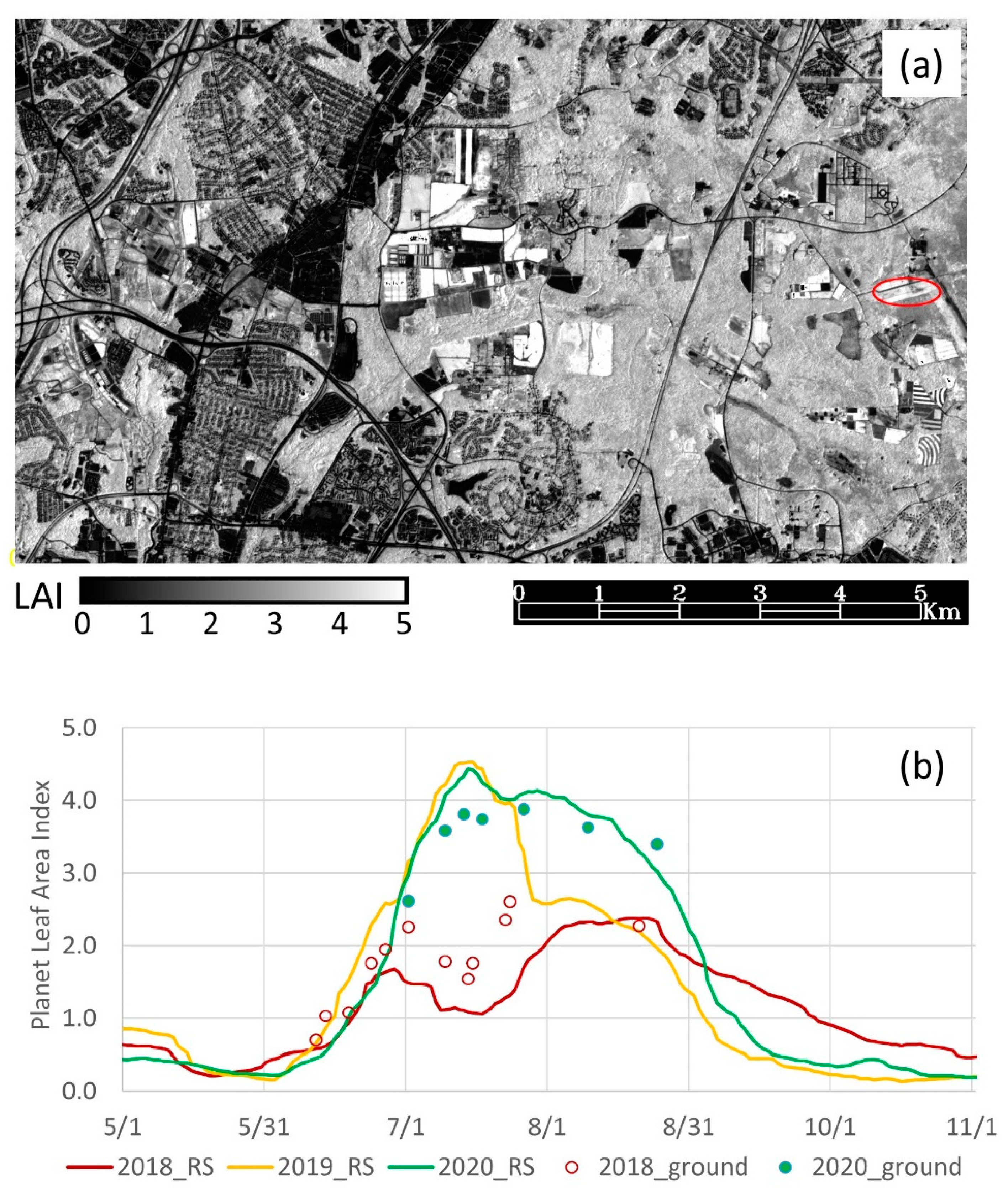
2.2. Remote-Sensing-Derived LAI and Phenology

2.2.1. Leaf Area Index

Leaf area index (LAI) was retrieved using a reference-based approach [49]. We used Sentinel-2 LAI as a reference to generate PlanetScope-based LAI at high spatial and temporal resolutions. The Sentinel-2 constellation includes 2A and 2B satellites which acquire optical imagery at 10–60 m spatial resolution collectively every 5 days [50]. The PlanetScope constellation consists of over 200 CubeSats in low earth orbits that can capture earth imagery daily at a 3 m resolution [51]. In order to generate daily LAI at a high spatial resolution, we combined Sentinel-2 LAI and Planet Fusion surface reflectance data using a machine learning approach, as described below.

Sentinel-2 L1C data were first downloaded and atmospherically corrected to the surface reflectance (L2A) using the Sen2Cor processor. Sentinel-2 surface reflectance was used to compute LAI at 10 m resolution using the Sentinel-2 Level 2 Prototype Processor (SL2P). Both atmosphere correction (Sen2Cor) and LAI retrieval (SL2P) processors are included in the European Space Agency (ESA) Sentinel Application Platform (SNAP) toolbox (https://earth.esa.int/eogateway/tools/snap, accessed on 13 May 2023). The Sentinel-2 LAI is retrieved using the artificial neural networks (ANNs) trained with radiative transfer model simulations [52]. Validation over croplands showed that Sentinel-2 LAI values were somewhat underestimated compared to “in situ” LAI for most crops (−0.37 for Sentinel-2 and −1.21 for Landsat) [53]. Seven clear Sentinel-2 images from 2019 and 2020 (8/29/2019, 9/8/2019, 11/2/2019, 1/21/2020, 4/15/2020, 6/9/2020, 7/14/2020) were selected and used to produce 10 m LAI over BARC. We included Sentinel-2 reference images from different seasons to capture the seasonal dynamics of vegetation.

Planet Fusion [54] constitutes a comprehensive fusion methodology based on the Cubesat Enabled Spatio-Temporal Enhancement Method (CESTEM) algorithm [55] to inter-calibrate, harmonize, and fuse multi-sensor data streams leveraging rigorously calibrated public mission (i.e., Sentinel-2, Landsat 8/9, Moderate Resolution Imaging Spectroradiometer (MODIS), Visible Infrared Imaging Radiometer Suite (VIIRS)) products in concert with the higher-spatial-and-temporal-resolution CubeSat images from the PlanetScope constellations. The Framework for Operational Radiometric Correction for Environmental Monitoring [56] generates a harmonized Sentinel-2 and Landsat 8/9 Bidirectional Reflectance Distribution Function (BRDF)-adjusted surface reflectance (SR) product that is used as the cross-calibration reference target during the radiometric harmonization step. Planet Fusion processing includes advanced temporally driven functionality related to radiometric and geometric harmonization, cloud and shadow masking, gap-filling, and temporal filtering to create analysis-ready data with high radiometric accuracy and spatio-temporal consistency. Planet Fusion delivers daily, 4-band (blue: 0.45–0.51 μm, green: 0.53–0.59 μm, red: 0.64–0.67 μm, and near infrared: 0.85–0.88 μm) surface reflectance data at 3 m spatial resolution.

Planet Fusion imagery acquired on seven cloud-free reference Sentinel-2 dates were resampled and used to build a combined training dataset at 10 m resolution. A data-driven machine learning approach (Cubist regression tree) was used to generate an LAI model by training the Sentinel-2 LAI and Planet Fusion surface reflectance at 10 m resolution. The trained regression tree model was applied to Planet Fusion data at the original 3 m resolution. The daily PlanetScope-based LAI was averaged for each field used in this study to generate field-level LAI from 2017 to 2021.

2.2.2. Crop Growth Stages

Crop growth stages were estimated using PhenoCam observations and Planet Fusion data. For the fields that contain installed PhenoCams, crop growth stages were visually interpreted using daily PhenoCam photos. This includes six maize and four soybean site years. Because some crop growth stages (especially reproductive stages) are hard to identify and differentiate using PhenoCam photos, the identified maize growth stages were limited to planting, tasseling (VT), silking (R1), maturity (R6), and harvest. For soybean growth stages planting, beginning bloom (R1), beginning maturity (R7), full maturity (R8), and harvest were identified based on the PhenoCam and other available digital images. These fields served as reference sites for the rest of the fields and years.

For target fields that did not contain PhenoCams, the two-band enhanced vegetation index (EVI2) computed from Planet Fusion data was used to estimate crop growth stages. The 2-band EVI2 approximates the 3-band enhanced vegetation index (EVI). EVI2 can be computed using surface reflectance from red and near-infrared (NIR) bands as:

$$\mathrm{EVI}2=2.5\ast \frac{\left(\mathrm{NIR}-\mathrm{red}\right)}{\left(\mathrm{NIR}+2.4\ast \mathrm{red}+1\right)}$$

(1)

We associated crop growth stages observed from PhenoCam reference sites with the EVI2 time series from the same field and year. Then, we compared the EVI2 time series from each target field to the reference sites using a dynamic time warping (DTW) technique [57]. The DTW measures the similarity between two non-linear time series. The reference site with the best match (smallest DTW distance) to the target site was selected. The dates of crop growth stages were retrieved using the warping path. For the fields without planting records, we used the within-season emergence (WISE) algorithm [47] to estimate crop emergence dates and then extrapolated planting dates utilizing the relationship between planting and emergence dates from reference sites.

2.3. DSSAT Model Description

The Decision Support System for Agro-technology Transfer (DSSAT) is a process-based crop model, evolved from the International Benchmark Sites Network for Agrotechnology Transfer Project [58,59,60,61]. DSSAT version 4.7.5 was used for this study. In order to simulate crop growth, development, and yield, the model requires a defined minimum dataset on weather, soil profiles, and crop management. The minimum weather dataset required to run the model includes maximum and minimum temperatures, solar radiation, wind speed, rainfall, and relative humidity. The soil parameters needed for the model include soil depth, and physical and chemical characteristics (i.e., drained lower limit, drained upper limit, saturation, and saturated hydraulic conductivity). In this study, soil profiles were obtained from the Soil Survey Geographic Database (SSURGO) (https://www.nrcs.usda.gov/resources/data-and-reports/soil-survey-geographic-database-ssurgo, accessed on 16 September 2021) and are provided in the supplementary file using the DSSAT soil profile file format (see Supplementary Table S1).

The model also requires crop management information such as crop type, cultivar, planting date, row and plant spacing, fertilizer application, tillage practices, and information on organic amendments for the fields or region [58,59,60,61]. In this study, two of the required crop variables (phenology and LAI) were not measured in most fields but were derived from the remotely sensed observations and subsequently used for model calibration and validation (see Section 2.2). Default cultivars were selected for the initial coefficient calibration based on the common cultivars planted or grown in the study area (see

Table 1. Starting (default) versus calibrated genetic cultivar coefficients for maize grown at BARC. Default cultivar: medium season.

Corn Genetic Coefficient	Description	Default Cultivar Value	Calibrated Value
P1	Thermal time from seedling emergence to end of juvenile phase (expressed in degree days above a base temp of 8 deg.C) during which the plant is not responsive to changes in the photoperiod.	200 (5–450) *	154.1
P2	The extent to which development is delayed for each hour increase in the photoperiod above the longest photoperiod at which development proceeds at max. rate (which is 12.5 h).	0.300 (0–2) *	0.001
P5	Thermal time from silking to physiological maturity (expressed in degree days above a base temp of 8 deg.C)	800 (580–999) *	592.7
G2	Maximum number of kernels per plant	700 (248–990) *	381.8
G3	Kernel filling rate during the linear grain filling state and under optimum condition (mg/day);	8.5 (5–16.5) *	15.31
PHINT	Phylochron interval; the interval in thermal time (degree days) between successive leaf tip appearances.	38.90 (38–49) *	49.00

* Note, values in parentheses are the ranges of the coefficients.

and

Table 2. Starting (default) versus calibrated genetic cultivar coefficients for soybean grown at BARC, production field. Maturity group 3.0 and 4.0 (MG3 and MG4).

Soybean Genetic Coefficient	Description	Default Value *	MG3	MG4
CSDL	Critical short day length below which reproductive development progresses with no daylength effect (for shortday plants) (hour)	13.09	12.00	12.98
PPSEN	Slope of the relative response of development to photoperiod with time (positive for shortday plants) (1/hour)	0.302	0.233	0.234
EM—FL	Time between plant emergence and flower appearance (R1) (photothermal days)	19.4	13.37	23.65
FL—SH	Time between first flower and first pod (R3) (photothermal days)	7.0	6.00	7.0
FL—SD	Time between first flower and first seed (R5) (photothermal days)	15.0	17.19	19.45
SD—PM	Time between first seed (R5) and physiological maturity (R7) (photothermal days)	34.00	37.60	37.67
FL—LF	Time between first flower (R1) and end of leaf expansion (photothermal days)	26.00	26.00	26.00
LFMAX	Maximum leaf photosynthesis rate at 30 C, 350 vpm CO2, and high light (mg CO2/m2/s)	1.030	1.038	1.006
SLAVR	Specific leaf area of cultivar under standard growth conditions (cm2/g)	375	340.7	356.8
SIZLF	Maximum size of full leaf (three leaflets) (cm2)	180.0	138.3	144.8
XFRT	Maximum fraction of daily growth that is partitioned to seed + shell	1.00	1.00	1.00
WTPSD	Maximum weight per seed (g)	0.19	0.161	0.165
SFDUR	Seed filling duration for pod cohort at standard growth conditions (photothermal days)	23.0	25.07	23.16
SDPDV	Average seed per pod under standard growing conditions (#/pod)	2.20	2.093	1.7401
PODUR	Time required for cultivar to reach final pod load under optimal conditions (photothermal days)	10.0	10.00	10.0
THRSH	Threshing percentage. The maximum ratio of (seed/(seed + shell)) at maturity. Causes seeds to stop growing as their dry weight increases until shells are filled in a cohort.	77.0	77.00	77.0
SDPRO	Fraction protein in seeds (g(protein)/g(seed))	0.405	0.405	0.405
SDLIP	Fraction oil in seeds (g(oil)/g(seed))	0.205	0.205	0.205

Note, the values are all within the ranges given by the model. Additionally, the cultivar traits in Table 2 include two daylength sensitivity traits (CSDL, PPSEN), five important life cycle “phase” durations (EM-FL, FL-SH, FL-SD, SD-PM, and FL-LF), some vegetative traits (SLAVR, SIZELF, EXFRT), and some reproductive traits (WTPSD, SFDUR, SDPDV, and PODUR). Variation in life cycle and duration of different phases is perhaps the most important genetic variation contributing to yield potential of different cultivars. * default for maturity group 4.

).

Daily weather data were obtained from the USDA Soil Climate Analysis Network (SCAN) station located at BARC, nearby to our study area (Powder Mill (2049), https://wcc.sc.egov.usda.gov/nwcc/site?sitenum=2049, accessed on 16 September 2021)). Weather variables used included daily maximum and minimum temperatures, solar radiation, wind speed, rainfall, and relative humidity. The data were quality controlled (i.e., missing values were filled with values from nearby stations or other data sources, and outliers were removed) before the DSSAT weather file format was created.

2.4. Model Calibration

To apply the DSSAT model in a particular location, one typically has to first run the model over a time period before the target application to calibrate key model parameters, such that it will reproduce, on average, the measured or reference growth and yield in most situations. One such key parameter set includes the cultivar coefficients which determine crop growth, development, and yield. To calibrate the model cultivar coefficients, crop information such as phenology, LAI, and yield are critical. This is because the calibration process entails fitting the model to measured or reference variables and where these variables are not measured, the model cannot be calibrated or adapted to the local agronomic conditions. Therefore, we need to estimate the set of parameter values that can accurately reproduce measured growth and yield. In our study, we used 17 treatments (site years) for maize (10 treatments as the calibration dataset, and seven treatments as the validation dataset). For soybean (maturity groups three and four), a total of 18 treatments (site years) were used (nine treatments as the calibration dataset, and nine treatments as the validation dataset) from the 2017 to 2020 period.

For the calibration of cultivar coefficients, it is known that if water, nutrients or other stresses affect experiments or trials (the crop data used for calibration), the estimate of cultivar coefficients may be poor [58,59,60,61]. Thus, we carefully selected our calibration treatments to include a range of weather conditions, day lengths, and crops growing in a minimum-stress or stress-free environment for the best results. Note that using data from multiple years/sites generates coefficients that are more robust. For this study, the treatments selected for calibration were based on the best selection criteria described above. We used the data described from Section 2.1, Section 2.2 and Section 2.3 as input to our model for calibration, including a combination of the field observations and remote sensing-derived parameters. We used all available crop management (seeding rates, fertilizer and irrigation applications, etc.), soil physical characteristics, and climate information (maximum and minimum temperature, precipitation, solar radiation, wind and relative humidity) data as model inputs [62].

We used the Generalized Likelihood Uncertainty Estimation (GLUE) tool in the DSSAT model for our initial calibration of cultivar coefficient for both maize and soybean cultivars. The GLUE procedures required two passes: the first pass estimates phenological parameters, and the second pass estimates growth and yield parameters. The remotely sensed LAI and phenological variables were key in our cultivar coefficients estimation, supporting model calibration and evaluation even though these variables were not measured in the field. The derived remote sensing and field variables were used for fitting the model to measured or reference variables. The cultivar coefficients were carefully calibrated with the field and remotely sensed observable crop variables such as phenology, LAI, and yield. We used more than 6000 runs to generate random sets of parameters based on prior distribution of the known genetic coefficients to generate our calibrated cultivar coefficients [63]. We then manually refined our results where necessary based on DSSAT calibration criteria in order to simulate the measured or reference results of the maize and soybean for our study [58,63]. The calibrated genetic cultivar coefficients for maize and soybean are listed in Table 1 and Table 2.

2.5. Model Evaluation

The agreement between the observed and simulated crop parameters was analyzed using the coefficient of determination (R²), which describes the proportion of the total variance explained by the model, as well as Willmott’s statistics measures [64,65] which include the index of agreement (d), which measures the degree to which simulated values match the observed values, the root mean squared error (RMSE), which is the sum of the differences between simulated and the observed values, and the normalized root mean squared error (NRMSE), which is a measure of the relative difference (%) between model-simulated and observed values (see the details of the index descriptions, equations and rating in [62]. We also used percentage difference (PD) for our analysis of the model, calculated as:

$$\mathrm{PD}=\frac{100\left({\mathrm{S}}_{\mathrm{i}}-{\mathrm{O}}_{\mathrm{i}}\right)}{{\mathrm{O}}_{\mathrm{i}}}$$

(2)

where S_i and O_i are the simulated and observed or reference values of a given variable, respectively. Lower PD indicates better model performance.

3. Results and Discussion

3.1. Remote Sensing LAI and Phenology Results

Figure 3 shows the map of the PlanetScope-based LAI on 1 August 2020, and the time series of LAI for the field 6-60 from 2018 to 2020. The remote-sensing-retrieved LAI at the field level was assessed using in situ LAI measurements collected in 2018 and 2020. Figure 3 shows that remote-sensing-retrieved LAI (field average) agrees well with field measurements (points) and follows a similar temporal pattern. The mean differences between remote-sensing-retrieved LAI and field measurements for the field 6-60 were −0.54 in 2018 and 0.27 in 2020, which is in the range of Sentinel-2 LAI retrieval accuracy for crops [53]. The daily PlanetScope-based LAI field averages were used as a parameter for the calibration and evaluation of our model. Note that the Planet team is developing an LAI data product (Planet Fusion LAI) using Planet Fusion surface reflectance. The Planet Fusion LAI can be used directly in this study once it becomes available. In this paper, we used the Sentinel-2 LAI as a reference to retrieve PlanetScope-based LAI, which is different from the Planet Fusion LAI by the Planet team.

The estimated crop growth stages were assessed using the leave-one-out cross-validation approach. We found that crop growth stages estimated from the Planet Fusion time series agreed well with the PhenoCam interpreted dates. The average absolute difference between the two was within one week from planting to maturity for both maize and soybean (see Supplementary Table S2). The harvest dates vary from year to year depending on management purposes; however, the remotely sensed harvest dates were not used in the DSSAT calibration process. The DSSAT model was set up to harvest at physiological maturity for both maize and soybean. Considering the uncertainty of photo interpretation, the accuracy of crop growth stages can satisfy the requirement for crop modeling. We used these derived growth stages for our model calibration and evaluation.

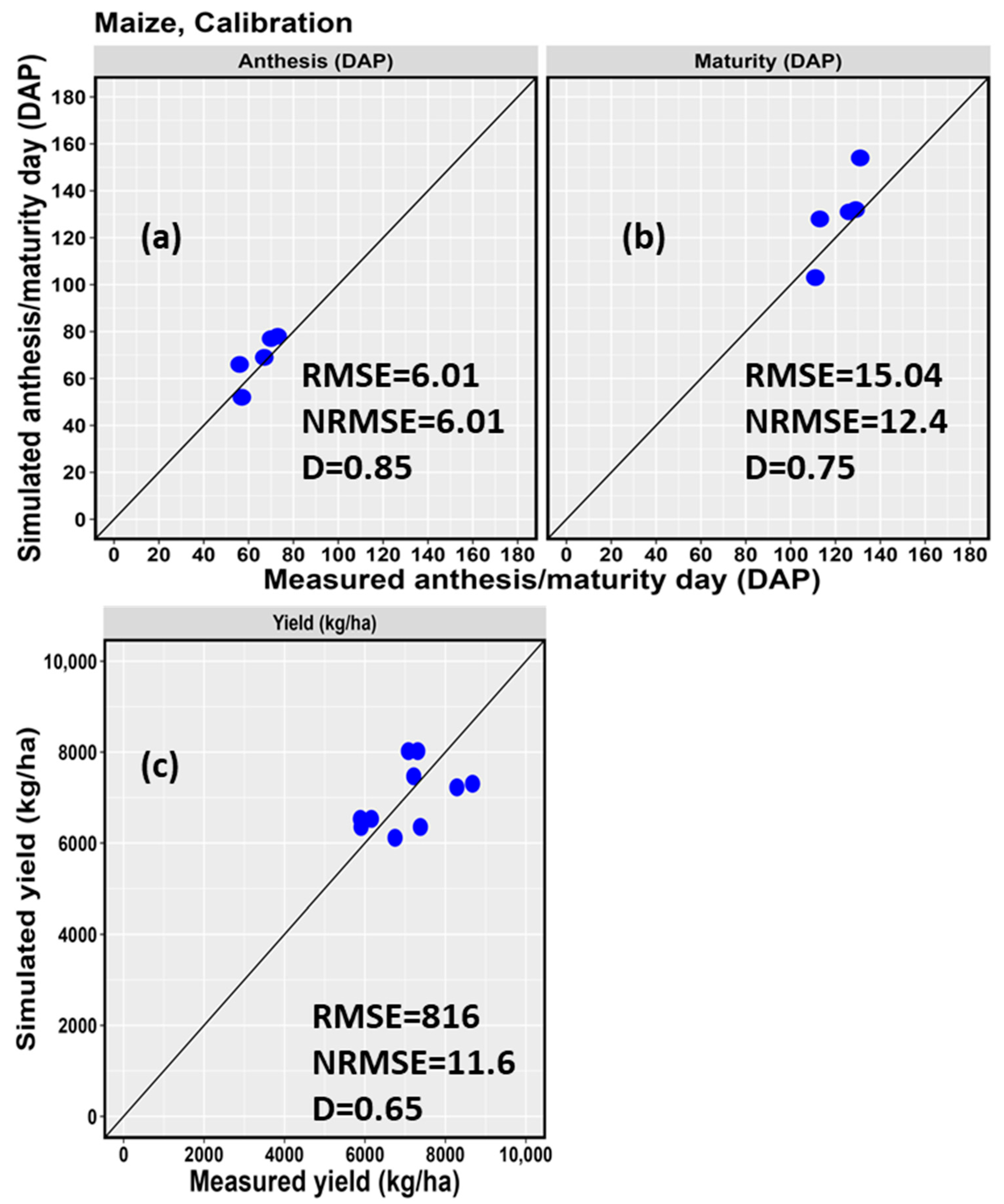
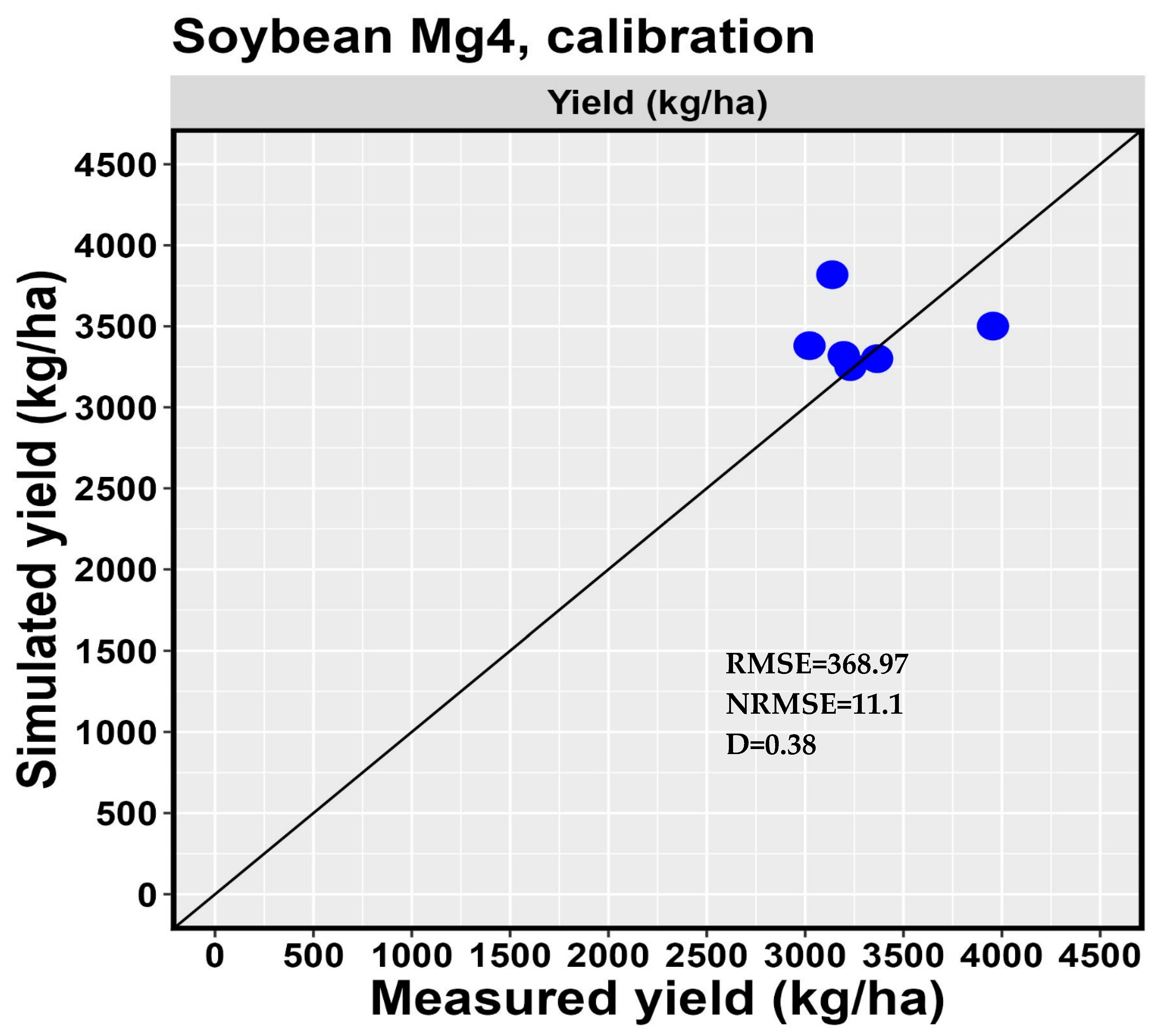
3.2. Model Calibration Results

Table 3. Calibration results for maize cultivars at BARC, Beltsville, Maryland.

	Field Info	Days to Flowering (R1)			Days to Maturity (R6)			Yield (kg/ha)
Field	Year	Obs	Sim	dev (%)	Obs	Sim	dev (%)	Obs	Sim	dev (%)
5-3B	2017	57	52	−8.8	111	103	−7.2	6160	6531	6.0
5-3B	2019	56	66	17.9	113	128	13.3	7378	6353	−13.9
5-3B	2020	67	69	3.0	131	154	17.6	7312	8021	9.7
5-3C	2017	57	52	−8.8	111	103	−7.2	6748	6115	−9.4
5-3C	2020	67	69	3.0	131	154	17.6	8674	7304	−15.8
5-3D	2017	57	52	−8.8	111	103	−7.2	5886	6531	11.0
5-3D	2019	56	66	17.9	113	128	13.3	5903	6353	7.6
5-3D	2020	67	69	3.0	131	154	17.6	7080	8021	13.3
2-71	2019	73	78	6.9	129	132	2.3	7213	7467	3.5
5-23	2019	70	77	10.0	126	131	4.0	8286	7224	−12.8
d		0.85			0.75			0.65
RMSE		6.01			15.04			816
NRMSE (%)		9.6			12.4			11.6

Note, Obs = observed, Sim = simulated, dev = deviation, R6 = physiological maturity. D = index of agreement, RMSE = root-mean-square error; NRMSE = normalized root-mean-square-error. Ratings are as follows: Excellent, NRMSE < 10% of mean observed; Good, 10% < NRMSE < 20%; Satisfactory, 20% < NRMSE < 30%; Unsatisfactory, NRMSE > 30% (Threshold based on the recommendation by [66,67]). Very good, d ≥ 0.9; Good, d ranges between 0.80–0.89; Moderate good, d ranges between 0.65–0.79; Moderately poor, d ranges between 0.50–0.64; Poor, d ranges between 0.25–0.49; Very poor, d < 0.25 (Threshold based on [65]).

and Figure 4 present the results for flowering and physiological maturity dates, and for the final grain yield of maize for the calibration dataset for 10 site years at BARC. The results are within 9.6 to 12% NRMSE of observations, which indicates that the calibrated model was able to estimate phenology and grain yield reasonably well for most of the fields analyzed. The Willmott’s statistics show a good agreement between the simulated and the observed yield (0.65 to 0.85). The results of the RMSE are reasonably low, especially for the flowering and grain yield of maize at BARC. These results demonstrated that remotely sensed derived parameters can be used to augment field observations, especially in data-poor regions. Additionally, these results are consistent with the conclusion of previous studies that integrating remote sensing with field observations as inputs to crop growth models provides an effective solution for assessing crop growth conditions and yield in data-poor regions [18,19,20,40].

For the soybean maturity groups 3 and 4,

Table 4. Calibration results for soybean maturity group 3 cultivars at BARC, Beltsville, Maryland.

	Field Info	Days to Flowering (R1)			Days to Maturity (R6)			Yield (kg/ha) *
Field	Year	Obs	Sim	dev (%)	Obs	Sim	dev (%)	Obs	Sim	dev (%)
5-3a	2018	41	41	0.0	128	121	−5.79	2937	3145	6.6
1-11	2019	37	38	2.6	93	101	7.92	*
1-34	2019	52	48	−8.3	124	128	3.13	*
2-51	2019	45	48	6.3	119	129	7.75	*
d		0.93			0.90
RMSE		2.55			7.57
NRMSE (%)		5.8			6.5

Note, Obs = observed, Sim = simulated, dev = deviation, R7 = Physiological maturity, * observed yield data missing so not evaluated. D = Index of agreement, RMSE = root-mean-square error; NRMSE = normalized root-mean-square error. Ratings are as follows: Excellent, NRMSE < 10% of mean observed; Good, 10% < NRMSE < 20%; Satisfactory, 20% < NRMSE < 30%; Unsatisfactory, NRMSE > 30% (Threshold based on the recommendation by [66,67]). Very good, d ≥ 0.9; Good, d ranges between 0.80–0.89; Moderate good, d ranges between 0.65–0.79; Moderately poor, d ranges between 0.50–0.64; Poor, d ranges between 0.25–0.49; Very poor, d < 0.25 (Threshold based on [65]).

and

Table 5. Calibration results for soybean maturity group 4 cultivars at BARC, Beltsville, Maryland.

	Field Info	Days to Flowering (R1)			Days to Maturity (R6)			Yield (kg/ha) *
Field	Year	Obs	Sim	dev (%)	Obs	Sim	dev (%)	Obs	Sim	dev (%)
8-15	2018	49	48	−2.04	120	117	−2.5	3230	3251	0.7
1-6	2018	47	47	0.00	126	116	−7.9	3955	3501	−11.5
1-6	2020	50	50	0.00	118	125	5.9	3366	3300	−2.0
NH-2	2018	48	47	−2.08	120	116	−3.3	3196	3320	3.9
ND-5	2018	46	47	2.17	112	117	4.5	3022	3380	11.8
ND-5	2020	43	48	11.63	122	122	0.0	3138	3818	21.7
d		0.58			0.34			0.38
RMSE		2.16			5.76			368.97
NRMSE (%)		4.6			4.8			11.1

Note, Obs = observed, Sim = simulated, dev = deviation, R7 = Physiological maturity, * observed yield data missing so not evaluated. D = Index of agreement, RMSE = root-mean-square error; NRMSE = normalized root-mean-square error. Ratings are as follows: Excellent, NRMSE < 10% of mean observed; Good, 10% < NRMSE < 20%; Satisfactory, 20% < NRMSE < 30%; Unsatisfactory, NRMSE > 30% (Threshold based on the recommendation by [66,67]). Very good, d ≥ 0.9; Good, d ranges between 0.80–0.89; Moderate good, d ranges between 0.65–0.79; Moderately poor, d ranges between 0.50–0.64; Poor, d ranges between 0.25–0.49; Very poor, d < 0.25 (Threshold based on [65]).

and Figure 5 and Figure 6 show the results of phenology (days to flowering and maturity) and yield for the calibration dataset for 4 site years (note, only one year of yield was available for maturity group three). The NRMSE ranged from 5 and 7%, indicating an excellent result for the phenology. This indicates that the calibrated model was able to estimate phenology reasonably well. However, the results of the Willmott’s statistics (d index) show a very good, calibrated model of soybean phenology for maturity group three but not for maturity group 4. Yield data for three out of the four fields planted in soybean maturity group three were not available; however, the field with available yield data showed an absolute deviation of 6.6%, which is very good. For the maturity group four, the model-simulated yield for the six calibrated fields did reasonably well (NRMSE of 16%).

Note that when the default model parameters were used, the results were very poor, as some fields could not reach maturity due to frost occurrence (results not shown). Calibration is critical to adapt DSSAT to local conditions.

3.3. Model Evaluation Results

Figure 7 and

Table 6. Evaluation (validation) results for maize cultivars at BARC, Beltsville, Maryland.

	Field Info	Days to Flowering (R1)			Days to Maturity (R6)			Yield (kg/ha)
Field	Year	Obs	Sim	dev (%)	Obs	Sim	dev (%)	Obs	Sim	dev (%)
5-3A	2017	57	52	−9.6	112	103	−8.7	8124	6466	−25.6
5-3A	2020	67	69	2.9	131	154	14.9	10,146	8318	−22.0
5-3C	2019	56	66	15.2	113	128	11.7	7051	7752	9.0
6-60	2018	65	61	−6.6	123	102	−20.6	4193	5281	20.6
6-60	2019	65	64	−1.6	122	120	−1.7	5692	7383	22.9
6-60	2020	66	69	4.3	123	154	20.1	9966	7946	−25.4
2-71	2020	64	69	7.2	130	144	9.7	10,890	6353	−9.8
D		0.72			0.53			0.82
RMSE		5.07			18.66			1495.34
NRMSE (%)		8.1			15.3			18.7

Note, Obs = observed, Sim = simulated, dev = deviation, R6 = Physiological maturity. D = Index of agreement, RMSE = root-mean-square error; NRMSE = normalized root-mean-square error. Ratings are as follows: Excellent, NRMSE < 10% of mean observed; Good, 10% < NRMSE < 20%; Satisfactory, 20% < NRMSE < 30%; Unsatisfactory, NRMSE > 30% (Threshold based on the recommendation by [66,67]). Very good, d ≥ 0.9; Good, d ranges between 0.80–0.89; Moderate good, d ranges between 0.65–0.79; Moderately poor, d ranges between 0.50–0.64; Poor, d ranges between 0.25–0.49; Very poor, d < 0.25 (Threshold based on [65]).

show the results of the flowering, physiological maturity, and the final grain yield of maize for the evaluation (validation) dataset for 7 site years at BARC. The days to flowering, maturity and final grain yield of maize were simulated with fairly good results (NRMSE < 20%) (Table 6). These results indicate that the simulated parameters strongly agreed with the measured or reference values (Figure 7 and Table 6). The deviation of the simulated from the observed evaluated parameters (flowering, maturity, and grain yield) for soybean maturity group three ranged between 1 and 8% (NRMSE,

Table 7. Evaluation results for soybean maturity group 3 cultivars at BARC, Beltsville, Maryland.

	Field Info	Days to Flowering (R1)			Days to Maturity (R6)			Yield (kg/ha) *
Field	Year	Obs	Sim	dev (%)	Obs	Sim	dev (%)	Obs	Sim	dev (%)
5-3B	2018	44	41	−6.8	123	121	−1.6	2731	3145	15.2
5-3C	2018	46	41	−10.9	121	122	0.8	2800	2913	4.0
5-3D	2018	43	41	−4.7	117	121	3.4	3022	3145	4.1
d		0.37			0.35			0.50
RMSE		3.56			2.65			257.74
NRMSE (%)		8.0			2.2			9.0

Note, Obs = observed, Sim = simulated, dev = deviation, R7 = Physiological maturity, * observed yield data missing so not evaluated. D = Index of agreement, RMSE = root-mean-square error; NRMSE = normalized root-mean-square error. Ratings are as follows: Excellent, NRMSE < 10% of mean observed; Good, 10% < NRMSE < 20%; Satisfactory, 20% < NRMSE < 30%; Unsatisfactory, NRMSE > 30% (Threshold based on the recommendation by [66,67]). Very good, d ≥ 0.9; Good, d ranges between 0.80–0.89; Moderate good, d ranges between 0.65–0.79; Moderately poor, d ranges between 0.50–0.64; Poor, d ranges between 0.25–0.49; Very poor, d < 0.25 (Threshold based on [65]).

), which indicates a very good, evaluated model. The model produced somewhat good results in some fields which is consistent with other evaluation studies [68]. The deviations from the observed values were larger for the maturity stage and grain yield of maize than for the flowering (Table 7). This is expected considering that it is harder to determine maturity based on the PhenoCam images which were used as a reference for the remotely-sensed derived phenology. Additionally, the yield monitor data show considerable variability of grain yields within the maize field ([48,69] see Figure 1a). However, our study used field averages for our calibration and evaluation (validation). For field 5-3A, the measured yield was unusually high (Table 6). Our investigation discovered that the field was heavily manured in the past, but this information was not adequately available to be captured during our calibration process. However, we subsequently added organic amendment in the management input file. A total of 2000 kg/ha of forage grass residue material was added. This improved our results, and the percent deviation between observed to simulated decreased. In addition, these results will be improved when more ground measurements become available to be used as a reference for the remotely sensed derived parameters (phenology and LAI) which were used as parameters for the calibration and evaluation of our model.

Overall, the evaluation (validation) statistics show that our calibrated models were able to simulate the observed or referenced parameters adequately which is consistent to the previous evaluation studies of the model [70]. Therefore, these calibrated models can be used in assessing the effects of climate change and adaptation option in this region, considering that the cultivars used in this study are common for the region. Additionally, these results show that remotely sensed crop information can be used to assess crop growth conditions and yield forecasting, especially when the needed parameters are not measured or are in a data-poor region.

For the soybean maturity groups three and four, Table 7 and

Table 8. Evaluation results for soybean maturity group 4 cultivars at BARC, Beltsville, Maryland.

	Field Info	Days to Flowering (R1)			Days to Maturity (R6)			Yield (kg/ha) *
Field	Year	Obs	Sim	dev (%)	Obs	Sim	dev (%)	Obs	Sim	dev (%)
8-15	2019	48	49	2.1	108	111	2.8	2663	2527	−5.1
8-15	2020	47	50	6.4	123	124	0.8	2371	3440	45.1
1-6	2019	50	49	−2.0	119	111	−6.7	2382	2182	−8.4
NH-2	2019	48	49	2.1	106	112	5.7	1915	2673	39.6
NH-2	2020	50	50	0.0	122	124	1.6	2411	3485	44.5
ND-5	2019	48	49	2.1	106	110	3.8	2394	2365	−1.2
d		0.48			0.88			0.15
RMSE		1.47			4.65			698.87
NRMSE (%)		3.0			4.1			29.7

Note, Obs = observed, Sim = simulated, dev = deviation, R7 = Physiological maturity, * observed yield data missing so not evaluated. D = Index of agreement, RMSE = root-mean-square error; NRMSE = normalized root-mean-square error. Ratings are as follows: Excellent, NRMSE < 10% of mean observed; Good, 10% < NRMSE < 20%; Satisfactory, 20% < NRMSE < 30%; Unsatisfactory, NRMSE > 30% (Threshold based on the recommendation by [66,67]). Very good, d ≥ 0.9; Good, d ranges between 0.80–0.89; Moderate good, d ranges between 0.65–0.79; Moderately poor, d ranges between 0.50–0.64; Poor, d ranges between 0.25–0.49; Very poor, d < 0.25 (Threshold based on [65]).

and Figure 8 and Figure 9 show the results of phenology (days to flowering and maturity) and yield over 4 and 6 site years for maturity groups three and four, respectively. The NRMSE ranges from 2 to 8%, indicating an excellent result for the phenology. The yield results indicated an excellent model (NRMSE of 1%, see Table 7) for maturity group three. For maturity group four, the results indicated satisfactory results (NRMSE of 30%). This is expected, owing to the fact that the management information was not readily available for maturity group four. This created uncertainties in many of our input data. In most cases, the cultivar numbers were not indicated in the management data record and assumptions were made about maturity group four basedF on the information available from other fields for the same year. In general, our results were consistent with the other evaluation studies of the model.

4. Conclusions

This paper assessed the integration of remotely sensed crop information and field observations to evaluate the DSSAT model in simulating soybean and maize growth and yield. The study demonstrated that remotely sensed crop variables such as LAI and phenology can be used for fitting model cultivar coefficients for yield estimation. The results show that the model’s comparison with the observed crop variables assessed produced a good result based on our limited range of data values in both the calibration and validation period. The model reasonably simulated measured soybean and maize phenology and produced a reasonable yield estimate, but not for all treatments. The evaluation of the model against the independent multi-year sites produced good results for phenology and somewhat good results for yield. Overall, the model performance with respect to phenology and grain yield was consistent with other evaluation studies of the model. These results show that remotely sensed crop information can be used to augment field observations for crop modeling, especially for data-poor regions or where no field records are available for modeling purposes.

References

1. Mutikani, L. Soybean Exports Power U.S. Economy to Best Performance in Two Years; Reuters: London, UK, 2016. [Google Scholar]
2. US Department of Agriculture, Economic Research Service (USDA-ERS). Ag and Food Statistics: Charting the Essentials; Administrative Publication: Beijing, China, 2018.
3. Campos, H.; Cooper, M.; Habben, J.; Edmeades, G.; Schussler, J. Improving drought tolerance in maize: A view from industry. Field Crop. Res. 2004, 90, 19–34. [Google Scholar] [CrossRef]
4. Hatfield, J.; Takle, G.; Groyjahn, R.; Holden, P.; Izaurralde, R.C.; Mader, T.; Marshall, E.; Liverman, D. Chapter 6: Agriculture. In Climate Change Impacts in the United States: The Third National Climate Assessment; Melillo, J.M., Terese, T.C.R., Yohe, G.W., Eds.; U.S. Global Change Research Program: Washington, DC, USA, 2014; pp. 150–174. [Google Scholar]
5. Dhakal, K.; Kakani, V.G.; Linde, E. Climate Change impact on wheat production in Southern Great Plains of the US using downscaled climate data. Atmos. Clim. Sci. 2018, 8, 143–162. [Google Scholar] [CrossRef]
6. IPCC. IPCC Special Report Onclimate Change, Desertification, Land Degradation, Sustainable Land Management, Food Security, and Greenhouse Gas Fluxes in Terrestrial Ecosytems; IPCC: Geneva, Switzerland, 2019. [Google Scholar]
7. Grigg, N.S. The 2011–2012 drought in the United States: New lessons from a record event. Int. J. Water Resour. Dev. 2014, 30, 183–199. [Google Scholar] [CrossRef]
8. Gowda, P.; Steiner, J.L.; Olson, C.; Boggess, M.; Farrigan, T.; Grusak, M.A. Agriculture and rural communities. In Impacts, Risks, and Adaptation in the United States: Fourth National Climate Assessment, Volume II; U.S. Global Change Research Program: Washington, DC, USA, 2018; pp. 391–437. [Google Scholar]
9. IPCC. Summary for policymakers. In Global Warming of 1.5 °C. An IPCC Special Report on the Impacts of Global Warming of 1.5 °C above Pre-Industrial Levels and Related Global Greenhouse Gas Emission Pathways, in the Context of Strengthening the Global Response to the Threat of Climate Change, Sustainable Development, and Efforts to Eradicate Poverty; Masson-Delmotte, V., Zhai, P., Pörtner, H.-O., Roberts, D., Skea, J., Shukla, P., Pirani, A., Moufouma-Okia, W., Péan, C., Pidcock, R., et al., Eds.; World Meteorological Organization: Geneva, Switzerland, 2018; p. 32. [Google Scholar]
10. Tilman, D.; Balzer, C.; Hill, J.; Befort, B.L. Global food demand and the sustainable intensification of agriculture. Proc. Natl. Acad. Sci. USA 2011, 108, 20260–20264. [Google Scholar] [CrossRef]
11. Ray, D.K.; Mueller, N.D.; West, P.C.; Foley, J.A. Yield trends are insufficient to double global crop production by 2050. PLoS ONE 2013, 8, e66428. [Google Scholar] [CrossRef] [PubMed]
12. Anderson, M.C.; Zolin, C.A.; Sentelhas, P.C.; Hain, C.R.; Semmens, K.; Yilmaz, M.T.; Gao, F.; Otkin, J.A.; Tetrault, R. The Evaporative Stress Index as an indicator of agricultural drought in Brazil: An assessment based on crop yield impacts. Remote Sens. Environ. 2016, 174, 82–99. [Google Scholar] [CrossRef]
13. FAO. The Future of Food and Agriculture-Trends and Challenges; FAO: Rome, Italy, 2017. [Google Scholar]
14. Huang, J.; Gomez-Dans, J.L.; Huang, H.; Ma, H.; Wu, Q.; Lewis, P.E.; Liang, S.; Chen, Z.; Xue, J.H.; Wu, Y.; et al. Assimilation of remote sensing into crop growth models: Current status and perspective. Agric. For. Meteorol. 2019, 276, 107609. [Google Scholar] [CrossRef]
15. Chipanshi, A.; Ripley, E.; Lawford, R. Large-scale simulation of wheat yields in a semi-arid environment using a crop-growth model. Agric. Syst. 1999, 59, 57–66. [Google Scholar] [CrossRef]
16. Moulin, S.; Guerif, M. Impacts of model parameter uncertainties on crop reflectance estimates: A regional case study on wheat. Int. J. Remote Sens. 1999, 20, 213–218. [Google Scholar] [CrossRef]
17. Wang, J.; Li, X.; Lu, L.; Fang, F. Estimating near future regional corn yields by integrating multi-source observations into a crop growth model. Eur. J. Agron. 2013, 49, 126–140. [Google Scholar] [CrossRef]
18. Kasampalis, D.A.; Alexandridis, T.K.; Deva, C.; Challinor, A.; Moshou, D.; Zalidis, G. Contribution of Remote Sensing on Crop Models: A Review. J. Imaging 2018, 4, 52. [Google Scholar] [CrossRef]
19. Li, Z.H.; Jin, X.L.; Zhao, C.J.; Wang, J.H.; Xu, X.G.; Wang Li, C.J.; Shen, J.X. Estimating wheat yield and quality by coupling the DSSAT-CERES model and proximal remote sensing. Eur. J. Agron. 2015, 71, 53–62. [Google Scholar] [CrossRef]
20. Levitan, N.; Kang, Y.; Ozdogan, M.; Maglillo, V.; Castillo, P.; Moshary, F.; Gross, B. Evaluation of the uncertainty in Satellite-Based crop state variable retrievals due to site and growth stage specific factors and their potential in coupling with crop growth models. Remote Sens. 2019, 11, 1928. [Google Scholar] [CrossRef]
21. Morel, J.; Begue, A.; Todoroff, P.; Martine, J.F.; Lebourgeois, V.; Petiti, M. Coupling a sugarcane crop model with the remotely sensed time series of FIPAR to optimize the yield estimation. Eur. J. Agron. 2014, 61, 60–68. [Google Scholar] [CrossRef]
22. Li, Y.; Zhou, Q.; Zhou, J.; Zhang, G.; Chen, C.; Wang, J. Assimilating remote sensing information into a coupled hydrology-crop growth model to estimate regional maize yield in arid regions. Ecol. Model. 2014, 291, 15–27. [Google Scholar] [CrossRef]
23. Dente, L.; Satalino, G.; Mattia, F.; Rinaldi, M. Assimilation of leaf area index derived from ASAR and MERIS data into CERES-Wheat model to map wheat yield. Remote Sens. Environ. 2008, 112, 1395–1407. [Google Scholar] [CrossRef]
24. Liang, S.; Qin, J. Data Assimilation Methods for Land Surface Variable Estimation, Advances in Land Remote Sensing, System, Modeling, Inversion and Applications; Liang, S., Ed.; Springer Science Business Media, BV: Berlin/Heidelberg, Germany, 2008; pp. 319–339. [Google Scholar]
25. Fang, H.; Liang, S.; Hoogenboom, G. Integration of MODIS LAI and vegetationindex products with the CSM-CERES-MAIZE model for corn yield estimation. Int. J. Remote Sens. 2011, 32, 1039–1065. [Google Scholar] [CrossRef]
26. de Wit, A.; Duveiller, G.; Defourny, P. Estimating regional winter wheat yield with WOFOST through the assimilation of green area index retrieved from MODIS observations. Agric. For. Meteorol. 2012, 164, 39–52. [Google Scholar] [CrossRef]
27. Ma, J.; Qin, S. Recent advances and developments of data assimilationalgorithms. Adv. Earth Sci. 2012, 27, 747–757. [Google Scholar]
28. Huang, J.; Tian, L.; Liang, S.; Ma, H.; Becker-Reshef, I.; Huang, Y.; Su, W.; Zhang, X.; Zhu, D.; Wu, W. Improving winter wheat yield estimation by assimilation of the leaf area index from Landsat TM and MODIS data into the WOFOST mode. Agric. For. Meteorolo. 2015, 204, 106–121. [Google Scholar] [CrossRef]
29. Wardlow, B.D.; Anderson, M.C.; Verdin, J.P. (Eds.) Remote Sensing for Drought: Innovative Monitoring Approaches; CRC Press/Taylor and Francis: Boca Raton, FL, USA, 2012. [Google Scholar]
30. Basso, B.; Cammarano, D.; Carfagna, E. Review of crop yield forecasting methods and early warning systems. In Proceedings of the First Meeting of the Scientific Advisory Committee of the Global Strategy to Improve Agricultural and Rural Statistics; FAO: Rome, Italy, 2013. [Google Scholar]
31. Rembold, F.; Atzberger, C.; Savin, I.; Rojas, O. Using low resolution satellite imagery for yield prediction and yield anomaly detection. Remote Sens. 2013, 5, 1704–1733. [Google Scholar] [CrossRef]
32. Liu, L.; Zhang, X.; Yu, Y.; Gao, F.; Yang, Z. Real-Time Monitoring of Crop Phenology in the Midwestern United States Using VIIRS Observations. Remote Sens. 2018, 10, 1540. [Google Scholar] [CrossRef]
33. Olson, D.; Chatterjee, A.; Franzen, D.W.; Day, S.S. Relation of drone-based vegetation indices with corn and sugarbeet yields. Agron. J. 2019, 111, 2545–2557. [Google Scholar] [CrossRef]
34. Diao, C. Remote sensing phenological monitoring framework to characterize corn and soybean physiological growing stages. Remote Sens. Environ. 2020, 248, 111960. [Google Scholar] [CrossRef]
35. Gao, F.; Anderson, M.C.; Johnson, D.M.; Seffrin, R.; Wardlow, B.; Suyker, A.; Diao, C.; Browning, D.M. Towards Routine Mapping of Crop Emergence within the Season Using the Harmonized Landsat and Sentinel-2 Dataset. Remote Sens. 2021, 13, 5074. [Google Scholar] [CrossRef]
36. Xu, W.; Jiang, H.; Huang, J. Regional Crop Yield Assessment by Combination of a Crop Growth Model and Phenology Information Derived from MODIS. Sens. Lett. 2011, 9, 981–989. [Google Scholar] [CrossRef]
37. Mishra, V.; Cruise, J.F.; Mecikalski, J.R. Assimilation of coupled microwave/thermal infrared soil moisture profiles into a crop model for robust maize yield estimates over Southeast United States. Eur. J. Agron. 2021, 123, 126–208. [Google Scholar] [CrossRef]
38. Shanahan, J.F.; Schepers, J.S.; Francis, D.D.; Varvel, G.E.; Wilhelm, W.W.; Tringe, J.M.; Schlemmer, M.R.; Major, D.J. Use of Remote-Sensing Imagery to Estimate Corn Grain Yield. Agron. J. 2001, 93, 583–589. [Google Scholar] [CrossRef]
39. Launay, M.; Guerif, M. Assimilating remote sensing data into a crop model to improve predictive performance for spatial applications. Agric. Ecosyst. Environ. 2005, 111, 321–339. [Google Scholar] [CrossRef]
40. Nearing, G.S.; Crow, W.; Thorp, K.; Moran, M.S.; Reichle, R.; Gupta, H. Assimilating remote sensing observations of leaf area index and soil moisture for wheat yield estimates: An observing system simulation experiment. Water Resour. Res. 2012, 48, W05525. [Google Scholar] [CrossRef]
41. LACIE. Proceedings of Plenary Session: The LACIE Symposium, NASA-JSC 14557; US Gov. Public Use Permitted: Houston, TX, USA, 1978.
42. Delécolle, R.; Maas, S.; Guérif, M.; Baret, F. Remote sensing and crop production models: Present trends. ISPRS J. Photogramm. Remote Sens. 1992, 47, 145–161. [Google Scholar] [CrossRef]
43. Bouman, B.A.M. Linking physical remote-sensing models with crop growth simulation-models, applied for sugar-beet. Int. J. Remote Sens. 1992, 13, 2565–2581. [Google Scholar] [CrossRef]
44. Bendig, J.; Yu, K.; Aasen, H.; Bolten, A.; Bennertz, S.; Broscheit, J.; Gnyp, M.L.; Bareth, G. Combining UAV-based plant height from crop surface models, visible, and near infrared vegetation indices for biomass monitoring in barley. Int. J. Appl. Earth Obs. Geoinf. 2015, 39, 79–87. [Google Scholar] [CrossRef]
45. Adão, T.; Hruška, J.; Pádua, L.; Bessa, J.; Peres, E.; Morais, R.; Sousa, J.J. Hyperspectral imaging: A review on UAV-based sensors, data processing and applications for agriculture and forestry. Remote Sens. 2017, 9, 1110. [Google Scholar] [CrossRef]
46. Zhou, X.; Zheng, H.B.; Xu, X.Q.; He, J.Y.; Ge, X.K.; Yao, X.; Cheng, T.; Zhu, Y.; Cao, W.X.; Tian, Y.C. Predicting grain yield in rice using multi-temporal vegetation indices from UAV-based multispectral and digital imagery. ISPRS J. Photogram. Remote Sens. 2017, 130, 246–255. [Google Scholar] [CrossRef]
47. Gao, F.; Anderson, M.; Daughtry, C.; Karnieli, A.; Hively, D.; Kustas, W. A within-season approach for detecting early growth stages in corn and soybean using high temporal and spatial resolution imagery. Remote Sens. Environ. 2020, 242, 111752. [Google Scholar] [CrossRef]
48. Dulaney, W.; Anderson, M.C.; Gao, F.; Daughtry, C.S.T.; Akumaga, U. Development of a Gridded Data Archive for Farm Management and Research at the USDA Beltsville Agricultural Research Center. Agrosyst. Geosci. Environ. 2023; in review process. [Google Scholar]
49. Gao, F.; Anderson, M.C.; Kustas, W.P.; Wang, Y. Simple method for retrieving leaf area index from Landsat using MODIS leaf area index products as reference. J. Appl. Remote Sens. 2012, 6, 063554. [Google Scholar] [CrossRef]
50. European Space Agency (ESA). Sentinel-2 User Handbook. 2015. Available online: https://sentinels.copernicus.eu/documents/247904/685211/Sentinel-2_User_Handbook (accessed on 13 May 2023).
51. Houborg, M.F. Daily Retrieval of NDVI and LAI at 3 m Resolution via the Fusion of CubeSat, Landsat, and MODIS data. Remote Sens. 2018, 10, 890. [Google Scholar] [CrossRef]
52. Weiss, M.; Baret, F. S2ToolBox Level 2 Products: LAI, FAPAR, FCOVER, 1.1. ed.; Institut National de la Recherche Agronomique: Avignon, France, 2016. [Google Scholar]
53. Djamai, N.; Fernandes, R.; Weiss, M.; McNairn, H.; Goïta, K. Validation of the Sentinel Simplified Level 2 Product Prototype Processor (SL2P) for mapping cropland biophysical variables using Sentinel-2/MSI and Landsat-8/OLI data. Remote Sens. Environ. 2019, 225, 416–430. [Google Scholar] [CrossRef]
54. Planet Labs, Planet Fusion Monitoring Technical Specification, Version 1.0.0-beta.3, 2021. Available online: https://assets.planet.com/docs/Planet_fusion_specification_March_2021.pdf (accessed on 13 May 2023).
55. Houborg, M.F. A Cubesat Enabled Spatio-Temporal Enhancement Method (CESTEM) utilizing Planet, Landsat and MODIS data. Remote Sens. Environ. 2018, 209, 211–226. [Google Scholar] [CrossRef]
56. Frantz, D. FORCE – Landsat + Sentinel-2 analysis ready data and beyond. Remote Sens. 2019, 11, 1124. [Google Scholar] [CrossRef]
57. Sakoe, H.; Chiba, S. Dynamic programming algorithm optimization for spoken word recognition. IEEE Trans. Acoust. Speech Signal Process. 1978, 26, 43–49. [Google Scholar] [CrossRef]
58. Jones, J.W.; Hoogenboom, G.; Porter, C.H.; Boote, K.J.; Batchelor, W.D.; Hunt, L.A.; Wilkens, P.W.; Singh, U.; Gijsman, A.J.; Ritchie, J.T. The DSSAT cropping system model. Eur. J. Agron. 2003, 18, 235–265. [Google Scholar] [CrossRef]
59. Hoogenbom, G.; Jones, J.W.; Porter, C.H.; Wilkens, P.W.; Boote, K.J.; Hunt, L.A.; Tsuji, G.Y. (Eds.) Decision Support System for Agrotechnology Transfer Version 4.5; University of Hawaii: Honolulu, HI, USA, 2010; Volume 1. [Google Scholar]
60. Hoogenboom, G.; Porter, C.H.; Boote, K.J.; Shelia, V.; Singh, U.; Wilkens, P.W.; White Pavan, W.; Oliveira, F.A.A.; Moreno-Cadena, L.P.; Lizaso, J.I.; et al. Decision Support System for Agrotechnology Transfer (DSSAT) Version 4.8 (DSSAT.net); DSSAT Foundation: Gainsville, FL, USA, 2021. [Google Scholar]
61. Hoogenboom, G.; Porter, C.H.; Boote, K.J.; Shelia, V.; Wilkens, P.W.; Singh, U.; White, J.W.; Asseng, S.; Lizaso, J.I.; Moreno, L.P.; et al. The DSSAT crop modeling ecosystem. In Advances in Crop Modelling for a Sustainable Agriculture; Burleigh Dodds Science Publishing: Cambridge, UK, 2019; pp. 173–216. [Google Scholar]
62. Hoogenboom, G.; Jones, J.W.; Traore, P.C.; Boote, K.J. Experiments and Data for Model Evaluation and Application., Improving Soil Fertility Recommendations in Africa Using the Decision Support System for Agrotechnology Transfer (DSSAT); Springer: Dordrecht, The Netherlands, 2012; pp. 9–18. [Google Scholar]
63. He, J.; Jones, J.W.; Graham, W.D.; Dukes, M.D. Influence of likelihood function choice for estimating crop model parameters using the generalized likelihood uncertainty estimation method. Agric. Syst. 2010, 103, 256–264. [Google Scholar] [CrossRef]
64. Willmott, C.J. Some comments on the evaluation of model performance. Bull. Am. Meteorol. Soc. 1982, 63, 1309–1313. [Google Scholar] [CrossRef]
65. Akumaga, U.; Tarhule, A.; Yusuf, A.A. Validation and testing of the FAO AquaCrop model under different levels of nitrogen fertilizer on rainfed maize in Nigeria, West Africa. Agric. For. Meteorol. 2017, 232, 225–234. [Google Scholar] [CrossRef]
66. Jamieson, P.D.; Porter, J.R.; Wilson, D.R. A test of the computer simulation model ARC-WHEAT1 on wheat crops grown in New Zealand. Field Crop. Res. 1991, 27, 337–350. [Google Scholar] [CrossRef]
67. Singh, J.; Knapp, H.V.; Demissie, M. Hydrologic Modeling of the Iroquois River Watershed Using HSPF and SWAT; ISWS CR 2004-08; Illinois State Water Survey: Champaign, IL, USA, 2004. [Google Scholar]
68. Araya, A.; Kisekka, I.; Gowda, P.H.; Prasad, P.V. Evaluation of water-limited cropping systems in a semi-arid climate using DSSAT-CSM. Agric. Syst. 2017, 150, 86–98. [Google Scholar] [CrossRef]
69. Kim, S.; Daughtry, C.; Russ, A.; Pedrera-Parrilla, A.; Pachepsky, Y. Analysis of Spatiotemporal Variability of Corn Yields Using Empirical Orthogonal Functions. Water 2020, 12, 3339. [Google Scholar] [CrossRef]
70. Araya, A.; Prasad, P.V.V.; Gowda, P.H.; Afewerk, A.; Abadi, B.; Foster, A.J. Modeling irrigation and nitrogen management of wheat in northern Ethiopia. Agric. Water Manag. 2019, 216, 264–272. [Google Scholar] [CrossRef]
Figure 1. Beltsville Agricultural Research Center (BARC) in Beltsville, Maryland showing average (a) maize yield and (b) soybean yields for our study fields for 2017–2020 from yield monitor system. The text beside the field represents the field name.
Agronomy 13 01540 g001
Figure 2. Phenocam images showing maize at R1 (anthesis) and R6 (maturity) stages in 2019 at field 5-3AB (labeled in Figure 1a).
Agronomy 13 01540 g002
Figure 3. PlanetScope-based LAI over BARC on 1 August 2020 (a) and LAI time series for the field 6-60 (old airport converted field, red circle in LAI map) from 2018 to 2020 (b). LAI ground measurements (points) from 2018 and 2020 (b) generally followed the LAI time series trend at the field level. In plot (a), the PlanetScope-based LAI map is scaled from 0 to 5 using a grayscale ramp.
Agronomy 13 01540 g003
Figure 4. The results of the simulated vs. observed (a) flowering (R1) (b) physiological maturity (R6) and (c) final grain yield for maize at BARC, DAP = day after planting.
Agronomy 13 01540 g004
Figure 5. The results of the simulated versus measured (a,b) flowering (R1) and (c,d) physiological maturity (R7) for soybean maturity groups 3 (Mg3) and 4 (Mg4) at BARC. DAP = day after planting, Mg = maturity group. Straight-line represent 1:1 line.
Agronomy 13 01540 g005
Figure 6. The results of the simulated versus measured yield for soybean maturity group 4 at BARC. Straight-line represent 1:1 line.
Agronomy 13 01540 g006
Figure 7. The evaluated maize results of the simulated versus observed (a) flowering (R1) (b) physiological maturity (R6) and (c) final grain yield at BARC. DAP = Day after planting. Straight-line represent 1:1 line.
Agronomy 13 01540 g007
Figure 8. The evaluated results of the simulated versus Observed (a,b) flowering (R1) (c,d) physiological maturity (R7), for soybean maturity group 3 and 4 at BARC. Straight-line represent 1:1 line.
Agronomy 13 01540 g008
Figure 9. The evaluated results of the simulated versus measured final grain yield for soybean maturity groups 3 and 4 at BARC. Mg = Maturity group. Straight-line represents 1:1 line.
Agronomy 13 01540 g009