Article

Tomato Leaf Disease Identification Method Based on Improved YOLOX

School of Electrical and Control Engineering, Shaanxi University of Science and Technology, Xi’an 710021, China
*
Author to whom correspondence should be addressed.
Agronomy 2023, 13(6), 1455; https://doi.org/10.3390/agronomy13061455
Submission received: 6 May 2023 / Revised: 23 May 2023 / Accepted: 23 May 2023 / Published: 25 May 2023
(This article belongs to the Special Issue Computer Vision and Deep Learning Technology in Agriculture)

Abstract

:
In tomato leaf disease identification tasks, the high cost and consumption of deep learning-based recognition methods affect their deployment and application on embedded devices. In this study, an improved YOLOX-based tomato leaf disease identification method is designed. To address the issue of positive and negative sample imbalance, the sample adaptive cross-entropy loss function (LBCE−β) is proposed as a confidence loss, and MobileNetV3 is employed instead of the YOLOX backbone for lightweight model feature extraction. By introducing CBAM (Convolutional Block Attention Module) between the YOLOX backbone and neck network, the model’s feature extraction performance is increased. CycleGAN is used to enhance the data of tomato disease leaf samples in the PlantVillage dataset, solving the issue of an imbalanced sample number. After data enhancement, simulation experiments and field tests revealed that the YOLOX’s accuracy improved by 1.27%, providing better detection of tomato leaf disease samples in complex environments. Compared with the original model, the improved YOLOX model occupies 35.34% less memory, model detection speed increases by 50.20%, and detection accuracy improves by 1.46%. The enhanced network model is quantized by TensorRT and works at 11.1 FPS on the Jetson Nano embedded device. This method can provide an efficient solution for the tomato leaf disease identification system.

1. Introduction

Crop diseases, a difficult problem plaguing agricultural production, severely restrict the sustainable development of agriculture [1]. Diseases and pests are the most challenging factors that decrease tomato yields [2,3]. Unfortunately, traditional tomato leaf disease identification relies mainly on professional judgement, which is inefficient and subjective. As a result, how to achieve efficient and accurate early identification and control of crop plant diseases has recently become a key research focus.
As deep learning has progressed, CNN (convolutional neural networks) have shown strong learning abilities in target identification applications [4,5,6,7] and have been applied to plant disease identification by many researchers [8,9,10,11]. For a wide range of plant diseases, CNN is well suited for extracting and classifying disease features, and the detection models can be better adapted to complex and changing field environments by improving the dataset [12,13,14]. In response to the above work, Karthik et al. [15] identified three types of tomato-diseased and healthy tomato leaves from 120,000 tomato leaf samples utilizing a deep residual network with an attention mechanism added to the neural network. According to the data, the model obtained 98% recognition accuracy in the experimental context.
The neural network model structure is overly complex, making it difficult to be ported to mobile platforms, and the field detection of plant diseases has high requirements for the model’s portability. There are some lightweight one-stage object detections at this point of development, such as the YOLO (you only look once) series of algorithms [16,17,18], SSD (single shot multiBox detector) [19], and RetinaNet. To create the detection result, the two-stage object detection first extracts the candidate region from the image and then performs secondary correction based on the candidate region, which has a slower detection speed yet a greater detection accuracy; the one-stage object detection algorithm calculates the image directly to provide the detection result, which has a quick detection speed but poor detection accuracy. Although one-stage object detection is more lightweight than two-stage object detection, there’s still much space for development. To address the above issues, there are some model light weighting efforts at this stage. Liu Yang et al. [20] used the PlantVillage open-source crop disease dataset as the research object and modified the network structure of the SqueezeNet to further lightweight the model. The improved model, with a model memory occupation of 0.62 MB, achieved an average accuracy of 98.13% and was suitable for embedded device deployment. Based on the improved AlexNet, Guo Xiaoqing et al. [21] developed a tomato leaf disease identification model that could be adapted to mobile platforms and created an Android-based tomato diseased leaves recognition system based on this model. The model used 29.9 MB of memory and had an average recognition accuracy of 92.70% for various times of tomato leaf disease. However, the recognition accuracy of the model could only reach 89.20% in practical situations, leaving much room for improvement.
Although one-stage object detection is faster, the number of candidate boxes that can match the target (positive samples) differs significantly from those that cannot (negative samples). This may result in an unbalanced positive and negative sample problem and affect the model’s training efficiency and detection accuracy. Tsung-Yi Lin et al. [22] addressed the problem of an excessive proportion of negative sample terms in the loss function. They improved the cross-entropy loss function by introducing adjustable parameters to change the proportion of positive and negative sample terms in the loss function. However, the parameters must be adjusted manually based on experience and training effects and cannot be adjusted adaptively. Li Xuefeng et al. [23] combined Dice loss with BCEloss to solve the sample imbalance problem by introducing Dice loss, but at the same time, it would reduce the model training efficiency.
Although the aforementioned studies achieved some model lightweighting achievements in various contexts, they do not have applications in embedded devices. That is, there is no guarantee of the practicality and feasibility of the models in real fields and under real conditions. To address the aforementioned issues, this research presents a YOLOX-S-based for tomato leaf disease detection. It can provide real-time field detection of tomato leaf disease. The following are the primary contributions of this paper:
(1)
A sample adaptive penalty coefficient is proposed, and a sample adaptive cross-entropy loss function is presented as the confidence loss of YOLOX.
(2)
A tomato leaf disease identification model based on YOLOX-MobileNetV3 is designed, allowing lightweight feature extraction.
(3)
The validated model was deployed on a Jetson Nano-embedded device. The model was shown to match the requirements for real-time, high-precision detection on embedded devices while also providing a viable option for tomato leaf disease identification.

2. Materials and Methods

The dataset was first determined in this study, and CycleGAN was used for data enhancement. Then an improved YOLOX-based tomato leaf disease identification method was designed, and a sample adaptive cross-entropy loss function was proposed. Next, comparative experiments were designed for the model, which included loss function comparison experiments, ablation experiments, and backbone comparison experiments, and the experimental data were obtained to be evaluated and analyzed to determine the benefits and disadvantages of the enhanced model. Suppose the experimental data show that the model can meet the application in practical situations. In that case, the model will be ported to an embedded system and mounted on an agricultural inspection robot to prove the practicality and feasibility of the model. Finally, tomato leaves collected in the field are used as the test set to verify the feasibility and practicality of the model. The complete procedure working flow is depicted in Figure 1.

2.1. Data Sources

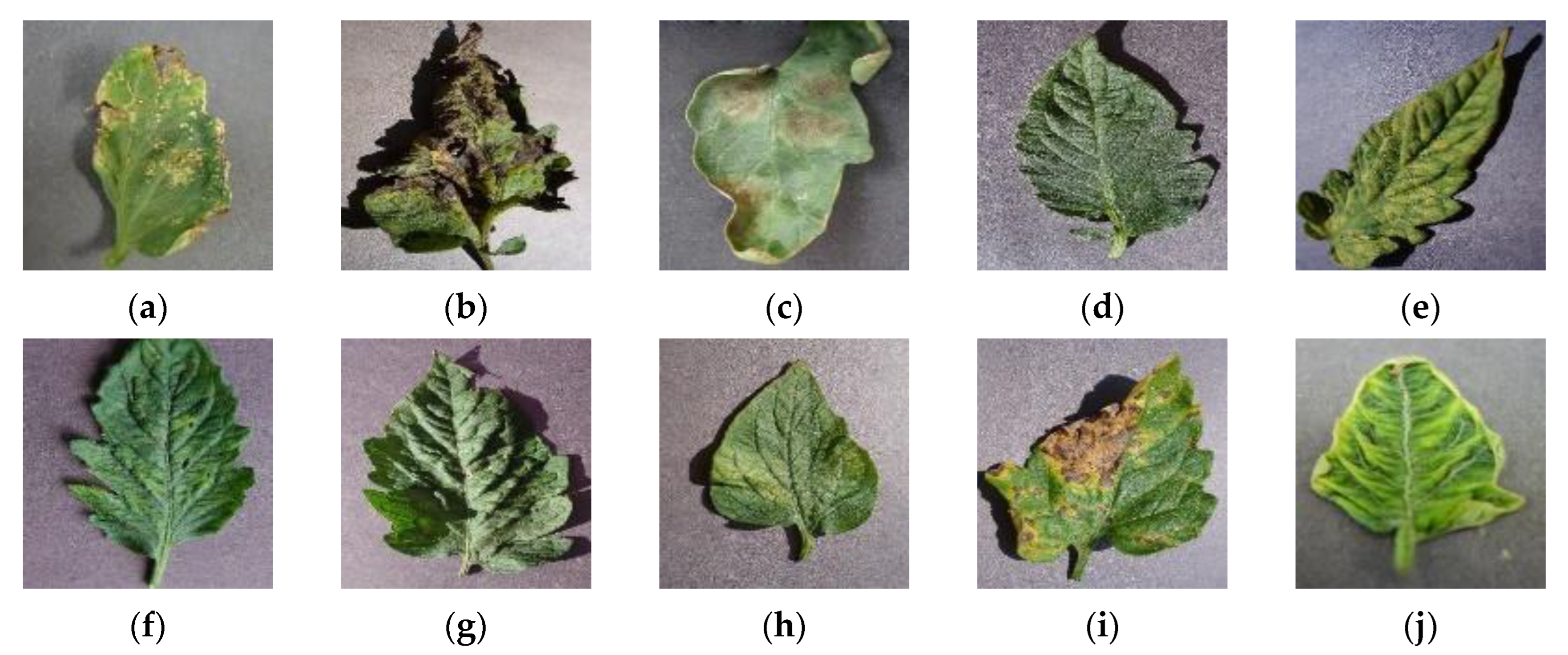
In this experiment, the PlantVillage dataset, which contained nine tomato disease leaf samples and healthy tomato leaf samples, was used, as shown in Figure 2. Table 1 depicts the distribution of samples in the dataset, with 18,834 images. The dataset was separated into three parts: training, testing, and validation, in a ratio of 8:1:1.
As the examples show, many tomato leaf diseases share similar traits, making it challenging to tell them apart from the naked eye. Furthermore, the different characteristics of tomato leaf diseases at different growth stages and the influence of external factors such as the background of the leaves, lighting, and leaf shadows when data are taken in realistic scenarios increase the difficulty of identifying tomato leaf diseases.

2.2. Data Enhancement

There is a problem with the unbalanced number of samples in the PlantVillage dataset, which reduces the recognition accuracy of the tomato leaf disease recognition model and may lead to overfitting. To resolve the issue of unbalanced samples in the dataset and achieve accurate identification and classification of the model, augmentation of samples with a small number of data is required. Data augmentation can be achieved through in-field data acquisition or the processing of existing data. In this study, the dataset’s average number of tomato leaf disease samples was 1883 per category. Data augmentation was performed using CycleGAN [24] for categories with less than 80% of the average value, augmenting early blight, leaf mold, mosaic virus, and target spot to 2000 samples and removing yellow leaf curl virus from similar samples and poor-quality samples to maintain a balance between the number of samples.
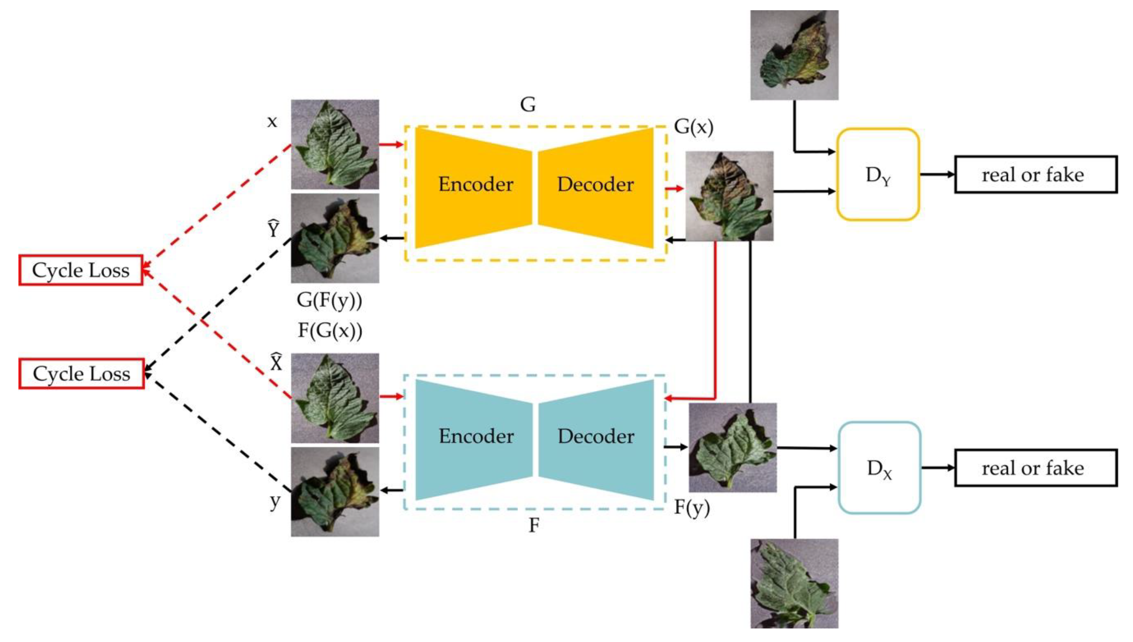
CycleGAN is a circular network model consisting of generative networks G and F and discriminators DX and DY. In this study, healthy tomato leaf data and less sample tomato leaf disease data are trained as input by CycleGAN, and the generative model can migrate the healthy tomato leaf sample style to the leaf disease tomato leaf sample style. The overall architecture of CycleGAN is shown in Figure 3.
CycleGAN maps the x domain to the target domain y via the generative network G, then restores from the target domain y via the generative network F. The y domain is mapped to the target domain x through the generative network F and then restored from the target domain x through the generative network G. The restored images are compared with the original domain images, forming a circular network. The transformation procedure from the source to the target domain is unknown if the GAN does not create a circular network, so the converted images may lose a significant number of original features and the generative networks G and F may overfit, which leads to the original domain being mapped to identical images in the target domain and the generated images being too monotonous. To retain the features of the original target domain to a greater extent, a loss function for cyclic consistency is introduced in the cyclic network, and the calculation formula is shown in (1):
L cyc ( G , F ) = E x ~ P d a t a ( x ) [ F ( G ( x ) ) x 1 ] + E y ~ P d a t a ( y ) [ G ( F ( y ) ) y 1 ]
where L cyc ( G , F ) is cyclic consistency loss function; x is x-domain image data; y is y-domain image data; P data ( x ) is x-domain image distribution; P data ( y ) is y-domain image distribution.
The discriminators’ D X and D Y can determine whether the input image is true or false. When the discriminator determines that the data generated by the input generative network is false, it releases a penalty to the generator, and the generative network learns in the direction of no penalty until the generative network generates data that the discriminator cannot determine to reach a balanced state. The calculation formula of the adversarial loss function is shown in (2):
L GAN ( G , D Y , X , Y ) = E y ~ P d a t a ( y ) [ log D Y ( y ) ] + E x ~ P d a t a ( x ) [ log ( 1 D Y ( G ( x ) ) ) ]
where L GAN ( G , D Y , X , Y ) is a one-way adversarial loss function from x to y; E y ~ P d a t a ( y ) is the expectation when y is subject to the P data ( y ) condition; E x ~ P d a t a ( x ) is the expectation when x is subject to the P data ( x ) condition.
The CycleGAN model can generate new leaf disease contour data based on healthy leaf contours and mimic disease features, enriching the generality of the training images. The number of augmented early blight, leaf mold, mosaic virus and target spot images are 2000 for each category. The results of the experiments show that the improved YOLOX detection model after CycleGAN data augmentation improves accuracy by 1.27% and provides better recognition of tomato leaf disease samples in complex situations.
The YOLOX algorithm includes the data enhancement function that performs operations on the dataset, such as random scaling, cropping, and ranking, after solving the sample balancing problem. When training, stop the data enhancement operation within the last 15 epochs. Table 1 shows the distribution of the number of samples after sample balancing and data enhancement.

2.3. Improved YOLOX Identification Method

2.3.1. Backbone Lightweighting

To reduce the model computation and improve its real-time performance, the CSPDarkNet53 is replaced by the lightweight network MobileNetV3 [25].
MobileNetV3 inherits the DSC (depthwise separable convolution) and inverted residual block proposed in MobileNetV1 and MobileNetV2 [26]. The DSC comprises depth-wise and pointwise convolution, with depthwise convolution convolving each input channel individually with independent convolution kernels. After convolution, the number of output channels equals the number of input channels. The result of the depthwise convolution is used as the input for pointwise convolution with 1 × 1 size kernel convolution again to achieve the purpose of reducing computation. Assuming a convolutional kernel of 3 × 3 size, DSC is 8–9 times less computationally intensive than normal convolution.
The nonlinear activation function can cause damage to low-latitude features. At the same time, the inverse residual structure first boosts the dimensionality with 1 × 1 convolution. Then it reduces the dimensionality with 1 × 1 convolution to decrease the damage of the nonlinear activation function to the original features and reduce the possibility of convolution kernel failure. The channel attention module SE [27] is also introduced in the inverted residual block of MobileNetV3, which improves the model learning ability for salient features.
In this paper, the YOLOX backbone is replaced with MobileNetV3-Large, whose network structure is shown in Table 2. In the table, input refers to the input size; bneck refers to the block cell in MobileNetV3; NBN refers to no batch normalization operation; exp size refers to the dimension boosted by the first layer of convolution; SE refers to whether the layer uses the SE attention mechanism; NL refers to the use of the HS (h-swish) or RE (ReLU) nonlinear activation function; s refers to the step size;—refers to the layer without the corresponding operation.

2.3.2. Loss Function Improvement

The YOLOX model is trained with the BCELoss function for category prediction and confidence prediction, and the expression of the BCELoss is shown in (3)–(4):
L i = y i log y i ( 1 y i ) l o g ( 1 y i ) = log y i y i = 1 log ( 1 y i ) y i = 0
L B C E = 1 N i = 1 N L i
where L i is the LBCE value generated at pixel i ; y i is the true label of pixel i , which takes the value of 1 for positive labels and 0 for negative labels, indicating the foreground object category and the background; y i is the predicted value of pixel i , taking values in the range [0, 1]; N is the total number of pixels in a batch.
The sample imbalance problem is usually solved by adjusting the structure of the loss function or the weights. Dice loss can improve the accuracy and reduce the imbalance between samples, but when the given data is extremely unbalanced, it can easily lead to gradient disappearance or explosion. Focal loss improves stability and robustness based on the cross-entropy loss function. However, its hyperparameters must be set and regulated according to experience, and it cannot achieve adaptive adjustment. The BCELoss function uses a category competition mechanism but cannot address the issue of data class imbalance. While tomato leaf diseases have a wide range of traits, and the characteristics of the same disease are not the same at different growth stages, there are similarities between different tomato leaf disease characteristics, which makes it difficult for the model to achieve the expected training effect.
To solve the aforementioned concerns, propose a sample adaptive penalty coefficient and design a sample adaptive cross-entropy loss function to automatically balance the weights of the loss function during model training based on the number of positive and negative samples fed in real-time without manual adjustment. The expressions of the sample adaptive penalty coefficient and the sample adaptive cross-entropy loss function are shown in (5)–(8):
α = arctan ( P + N P + δ ) y = 1 arctan ( P + N N + δ ) y = 0 , α [ 0 , π 2 ]
β = sin α , β [ 0 , 1 ]
B C E L o s s β = β y l o g y β ( 1 y ) l o g ( 1 y )
L B C E β = 1 1 + exp ( B C E L o s s β )
where β is the sample adaptive penalty coefficient; LBCE−β is the sample adaptive cross-entropy loss function; P is the total amount of positive samples for network training feedback; N is the total negative samples for network training feedback; δ is a minimal value.
The sample adaptive penalty coefficient can adaptively alter the weight of the loss function based on the number of positive and negative samples returned during model training. For example, when there is a limited quantity of positive samples, the β value of the y = 1 term increases and the β value of the y = 0 term decreases, and the positive sample’s feature loss weight grows while the negative sample’s feature loss weight drops. Conversely, when the quantity of negative samples is small, the negative sample feature loss weight is increased, and the positive sample feature loss weight is decreased. By discarding some of the gradients, the positive and negative samples are in dynamic equilibrium, and the loss function can automatically balance the positive and negative sample loss coefficient weights at all stages of the training process to iterate in its favor to achieve better training results. In addition, the sigmoid function activates the loss function to ensure that the output of the confidence loss value is within the interval [0, 1], which makes the gradient descent of the loss function more stable.

2.3.3. Improved Network Model Structure

Tomato leaf diseases have comparable characteristics among species. And the characteristics of leaf diseases are not the same at different stages, which leads to a more difficult tomato leaf disease identification task. In identifying tomato leaf disease, determining the disease category is more influenced by the background features, and knowing how to improve the extraction of disease feature location information becomes crucial. The YOLOX network, a one-stage object detection algorithm with fast detection speed, works as follows: first, the tomato leaf disease dataset is processed for data enhancement to reduce the possibility of model overfitting, and the epoch for data enhancement off can be set; second, the tomato leaf images are extracted for features by CSPDarkNet53; the extracted leaf disease features are fused with FPN and PAN to improve the learning of location and classification; and finally, to achieve classification and localization, the extracted leaf disease traits are decoupled with a decoupling head.
The YOLOX network model was employed as the core framework for detecting tomato leaf disease in this study, and the YOLOX network structure is shown in Figure 4.
The YOLOX neck network is a feature pyramid composed of two parts, FPN and PAN, which first fuse high-level characteristics with low-level characteristics by upsampling the FPN feature pyramid network and then reinforce the model’s learning ability for localization features by the PAN path aggregation network. Finally, the fused features are decoupled by the decoupling detection head, which is realized in Anchor-Free.
The YOLOHead part is the biggest improvement over the YOLO family of algorithms, with the prediction box removed from the head network and the decoupled approach to target class prediction used, enabling end-to-end detection. Similar applications are currently found in many one-stage networks, such as RetinaNet and FCOS, and this method eliminates the operation of non-maximal suppression in NMS. However, decoupling the detection head will improve the complexity of the computation and thus reduce the real-time performance of the model.
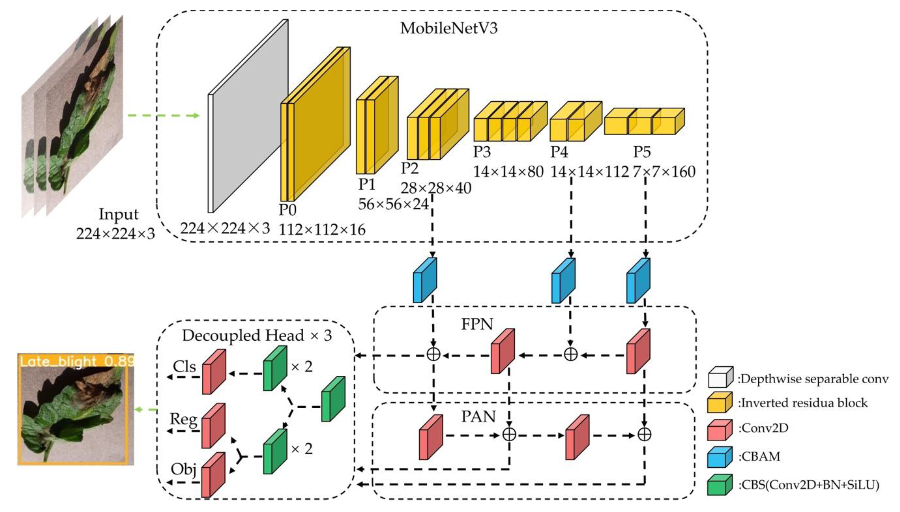
Figure 4 shows that the decoupling head has three branches, namely Cls, Reg, and Obj, where Cls is to classify the attributes in the target frame and predict the category probability. Reg is to predict the destination frame coordinate information. Finally, Obj is mostly responsible for determining if the target frame is in the foreground or background.
The overall network structure of the improved YOLOX model is shown in Figure 5. This study introduced a three-layer CBAM [28] between the backbone and the feature pyramid network. By allocating channel and spatial attention weights, background interference on feature extraction is reduced, and the model’s ability to extract tomato leaf disease features is improved. The backbone is also updated with MobileNetV3 to achieve lighter feature extraction and better real-time mobility of the model.

2.4. Model Training

2.4.1. Model Evaluation Indicators

The model evaluation metrics employ mAP (mean average precision, %) to assess the model’s correctness, FLOPs, and memory usage to evaluate the model’s usefulness, and the single-frame image recognition speed evaluates the real-time and recognition efficiency of the model.

2.4.2. Experimental Operating Platform

The model training part of this experiment will be conducted on the same computer with the following platform: CPU: 12th Gen Intel Core i5-12400F made in Chengdu, China, NVIDIA GeForce RTX 3060 GPU with 12GB of video memory and 16GB of running memory, OS: Ubuntu 20.04, Compiler tool: PyCharm, Framework: PyTorch 1.10.1 (with CUDA 11.3), Language: Python 3.7.4, Training dataset: COCO dataset, Dataset annotation tool: Eiseg 0.5.0, detection framework: MMDetection 2.0. This section may be divided into subheadings.

2.4.3. Parameter Settings

The experiments were trained in multiple batches, with the number of GPUs set to 1, the batch size set to 4, the epoch set to 30 rounds, the input image size set to 224 × 224 pixels, the image in RGB-mode JPG format, the optimizer SGD, the Learning rate set to 0.001, the weight decay factor set to 0.0005, and the momentum factor set to 0.937.

3. Results and Discussion

3.1. Analysis and Comparison of Results

3.1.1. Analysis of Identification Results

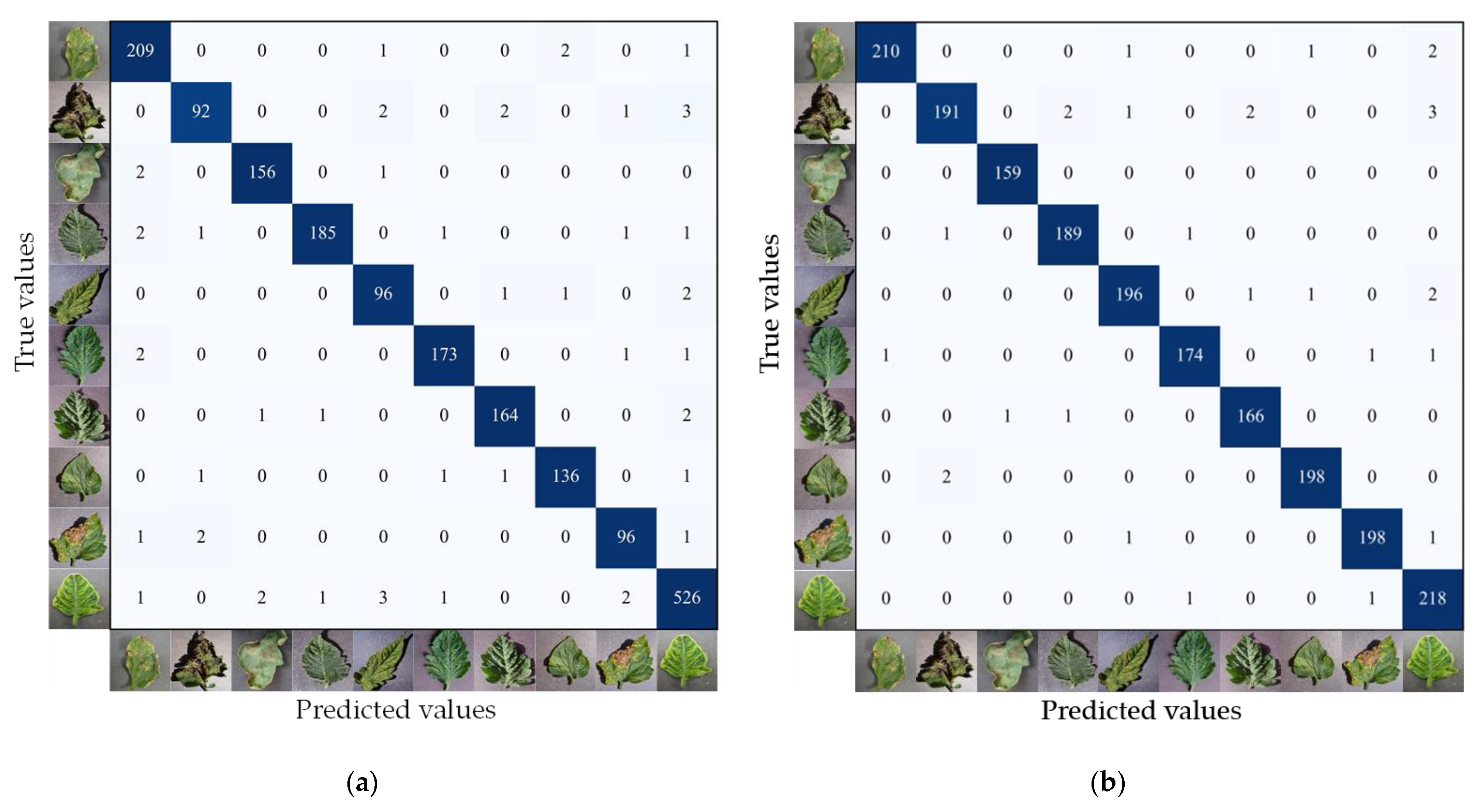
To demonstrate the results of the improved YOLOX more visually in terms of recognition accuracy and classification between samples in the tomato leaf disease dataset before and after sample balance, a confusion matrix was plotted based on the test set, as shown in Figure 6.
From the confusion matrix in Figure 6, it can be seen that the sample balanced tomato leaf disease recognition model improved the recognition accuracy of early blight by 3.98%, leaf mold by 2.00%, target spot by 1.86% and mosaic virus by 3.00% in the test set. It was demonstrated that when CycleGAN was used to enhance the dataset, it could effectively solve the problem of poor recognition accuracy of individual samples caused by unbalanced tomato leaf disease samples.
For the improved YOLOX detection model for all types of tomato diseases, recognition accuracy ranged from 95.98% to 100.00%, and the average recognition accuracy was 98.56%, which indicates that the improved detection model can perform better on the experimental data set and meet the requirements of recognition model accuracy.

3.1.2. Loss Function Comparison Experiments

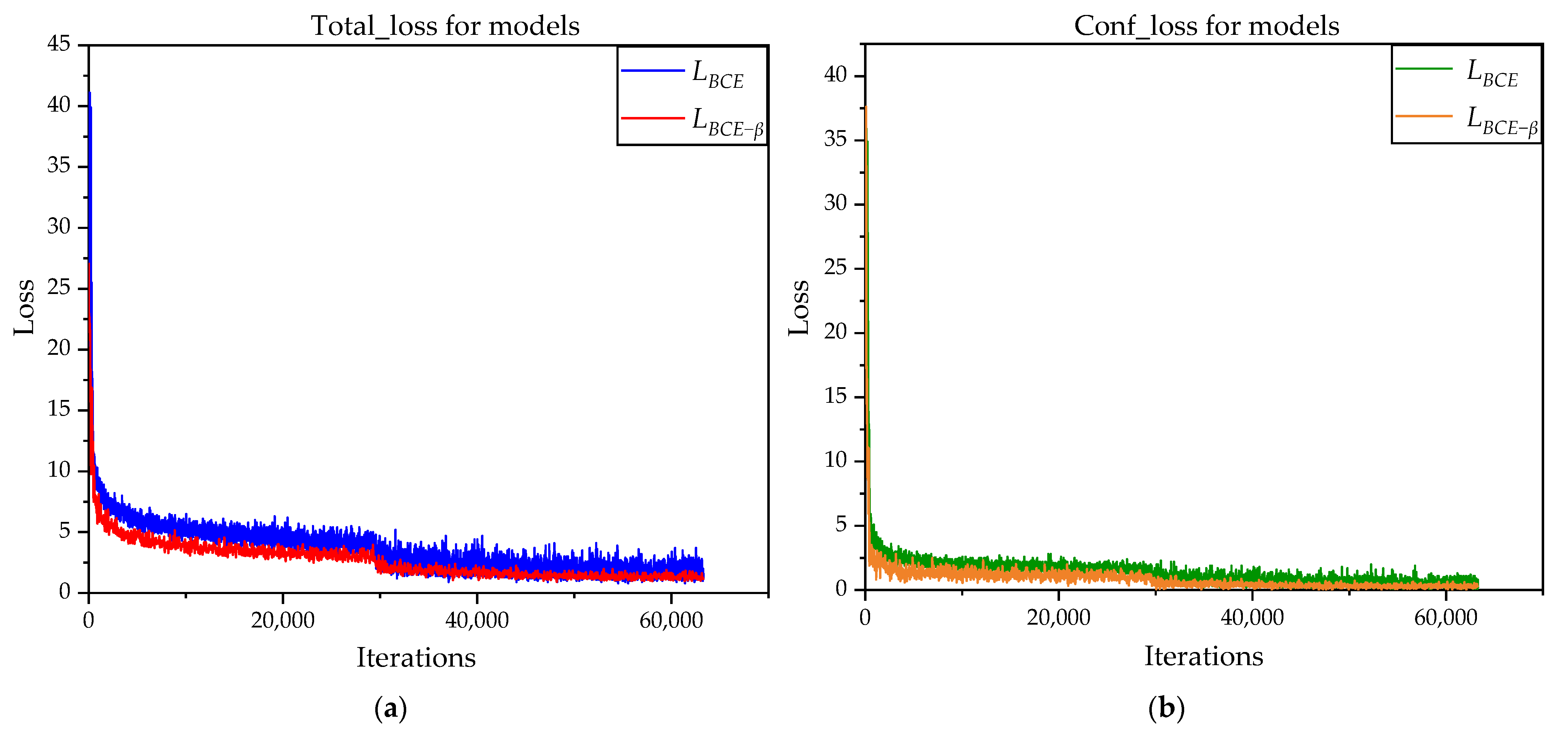
A comparison of the confidence loss function curves based on the YOLOX is shown in Figure 7. The curves compare the original YOLOX loss function LBCE with the sample adaptive loss function LBCE−β proposed in this paper.
The LBCE−β changes the positive and negative sample feature loss weights adaptively based on the number of positive and negative samples sent back during model training, and the curve converges faster than the loss function curve in the original YOLOX detection model. Furthermore, after convergence, the LBCE−β curve oscillates less than the initial loss function curve. The value of the loss function after convergence is lower than that of the original loss function, and the modified loss function is more stable after convergence, indicating that the LBCE−β can improve the model’s generalization ability.

3.1.3. Ablation Experiments

The ablation experiment verifies whether the module can improve the detection performance of the network model by keeping or removing certain network modules. This experiment verifies the effect of the CBAM attention mechanism module and the improved loss function on the model detection performance when YOLOX uses CSPDarkNet53 and MobileNetV3 as the backbone, and each performance metric is shown in Table 3.
The ablation experiment outcomes show that the introduction of the CBAM and the improved loss function have minimal influence on the FLOPS of the detection model, the memory usage, and the single-frame image recognition speed. The introduction of the CBAM increases the recognition accuracy by 0.52%. The improved loss function increases the recognition accuracy by 0.58% when using the CSPDarkNet53 backbone. The introduction of the CBAM improves the recognition accuracy by 0.86%, and the improved loss function improves the recognition accuracy by 1.71% when using the MobileNetV3 backbone network. Based on the findings of the experiments, it is clear that both the CBAM and the loss function module, with the introduction of sample adaptive penalty coefficients, have a beneficial effect on the recognition outcomes of the tomato leaf recognition model.
After replacing the YOLOX backbone with MobileNetV3, the FLOPS, memory usage, and single-frame image recognition speed are greatly improved. The results of the experiments reveal that the improved YOLOX has 35.34% less model memory, 50.20% higher model recognition speed, and 1.46% higher recognition accuracy compared to the original YOLOX, and the performance has been improved in all aspects.

3.1.4. Backbone Comparison Experiment

The improved YOLOX detection model is compared with the Faster RCNN [29] and the RetinaNet in the framework of MMDetection 2.0, and the model when using different backbone networks with the addition of the CBAM and improved loss function to the YOLOX performance is compared. Considering the need to port the model to an embedded platform in subsequent field detection work, which requires a sufficiently lightweight model, the lightweight networks GhostNet [30], EfficientNet [31], and MobileNetV3 are selected as the backbone networks of YOLOX, respectively. All three networks possess the benefits of less network settings and accelerated model inference. Table 4 shows the results of comparing YOLOX performance with various network architectures in different backbone networks.
As shown in Table 4, the Faster RCNN has the highest recognition accuracy of 98.77%, but the FLOPS and memory usage are too large, which makes the model less effective when ported to embedded devices and makes it challenging to implement field deployment applications. YOLOX-MobileNetV3 is more suitable for disease identification on tomato leaves in real-world applications, as it is 81.00% less computationally intensive, 85.95% less memory intensive and 5.23 times faster than the Faster RCNN network. However, the recognition accuracy is 0.21% less.
When YOLOX uses GhostNet as the backbone, the detection model takes up less memory. When YOLOX uses EfficientNet as the backbone, the model is less computationally intensive, but the recognition accuracy is poor. When MobileNetV3 was used as the backbone for YOLOX, the model’s accuracy was 0.74% higher than GhostNet, and the recognition speed was 28.52% faster than GhostNet, making the identification of tomato leaf diseases more accurate and efficient.

3.2. Tomato Leaf Disease Detection Effect in Embedded Devices

Traditional deep learning techniques are deployed using IPCs (industrial personal computers), but their weight and strength limit their ability to identify diseased tomato leaves in the field in real-time. The NVIDIA Jetson Nano is the most economical portable edge device, low-cost, and low-consumption for recognition tasks in the field.
The tomato leaf disease detection platform with the Jetson Nano as the master controller is shown in Figure 8. It comprises an agricultural inspection robot and a tomato leaf disease identification system. When the agricultural inspection robot performs inspection work, the tomato leaf disease detection system performs real-time identification work on the photographed tomato leaves. In addition, it retains information on the location of detected tomato leaf diseases for subsequent processing.
The Jetson Nano is used as the embedded deployment platform in this investigation. The software environment is set to TensorRT-7.1.3.0 and JetPack-4.4.1 and set the image input size to 224 by 224. TensorRT is used to quantify the correctness of the model parameters and to integrate the process so that the model runs as much as feasible on the GPU, allowing it to run faster. We tested the inference speed of YOLOX, improved YOLOX, and improved YOLOX based on TensorRT quantization on the Jetson Nano, and the results are shown in Table 5.
As can be seen in Table 5, YOLOX-MobilenetV3 runs faster than the original YOLOX on embedded devices, but both require a longer build time. The build phase consumption time is reduced by almost two times after FP32 TensorRT acceleration and almost five times after FP16 TensorRT acceleration, and the single-frame image detection time is reduced to 0.09 s, which can run at 11.1 FPS. The TensorRT-accelerated YOLOX-MobileNetV3 can address real-time demands for tomato leaf disease detection on embedded devices.
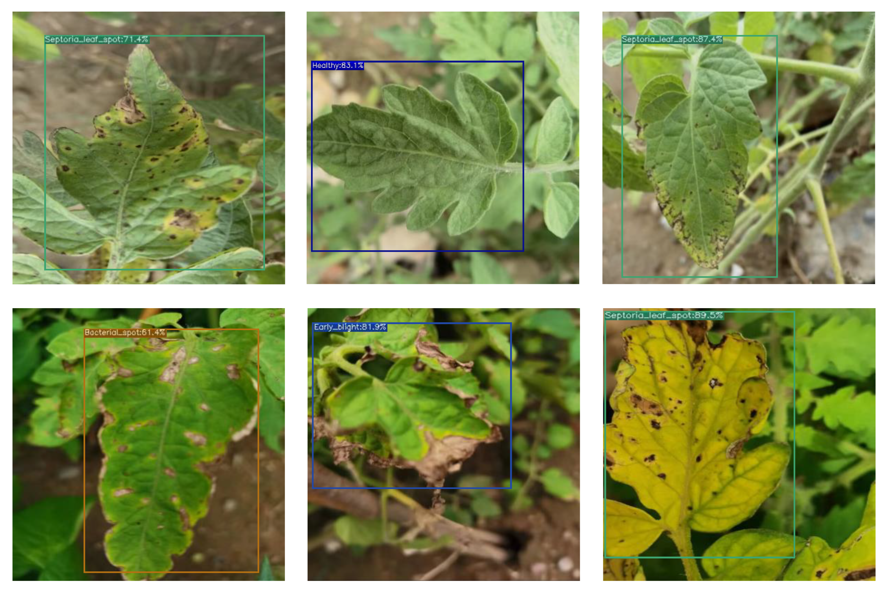
Tomato leaves collected in the field were used as the test set to validate the improved YOLOX, and the recognition results are displayed in Figure 9. The results of the recognition show that the model has good detection rates in real-life situations with complex backgrounds and is better able to meet the needs of practical applications.

4. Conclusions

This paper describes an improved YOLOX approach for identifying tomato leaf diseases to address the issue of data imbalance in tomato disease leaf samples and the need for model lightweighting in practical circumstances. To address the issue of positive and negative sample imbalance in a one-stage target detection method, we present a sample-adaptive cross-entropy loss function. We also replace the backbone of YOLOX and propose the YOLOX-MobileNetV3 target detection algorithm to achieve model feature extraction lightweighting. CBAM is used between the backbone of YOLOX and the neck network to improve the model feature extraction capability. Some dataset samples are processed by CycleGAN before model training to address the imbalanced sample size in the dataset.
After simulation experiments and physical validation, the improved YOLOX detection model has improved recognition speed, accuracy, and memory usage. The model has better detection results in the context of complex reality situations, which can better achieve the needs of applications in real life and serve as references for the identification of tomato leaf disease in greenhouses or the construction of tomato leaf disease recognition systems based on embedded platforms.

Author Contributions

Conceptualization, W.L.; methodology, W.L. and Y.Z.; software, Y.Z.; validation, Y.Z. and Y.X.; formal analysis, W.L. and Y.Z.; investigation, W.L.; resources, W.L. and Y.X.; data curation, Y.Z.; writing—original draft preparation, W.L. and Y.Z.; writing—review and editing, W.L., Y.Z. and Y.X.; visualization, W.L.; supervision, W.L. and Y.X.; project administration, W.L. and Y.Z.; funding acquisition, W.L. and Y.X. All authors have read and agreed to the published version of the manuscript.

Funding

This research was funded by the National Natural Science Foundation of China Youth Program (62203285); Shaanxi Province Natural Science Basic Research Program Funding Project (2022JQ-181).

Data Availability Statement

Conflicts of Interest

The authors declare no conflict of interest.

References

  1. Hassan, S.M.; Jasinski, M.; Leonowicz, Z.; Jasinska, E.; Maji, A.K. Plant Disease Identification Using Shallow Convolutional Neural Network. Agronomy 2021, 11, 2388. [Google Scholar] [CrossRef]
  2. Fuentes, A.; Yoon, S.; Kim, S.C.; Park, D.S. A robust deep-learning-based detector for real-time tomato plant diseases and pests recognition. Sensors 2017, 17, 2022. [Google Scholar] [CrossRef] [PubMed]
  3. Xiong, Y.; Liang, L.; Wang, L.; She, J.; Wu, M. Identification of cash crop diseases using automatic image segmentation algorithm and deep learning with expanded dataset. Comput. Electron. Agric. 2020, 177, 105712. [Google Scholar] [CrossRef]
  4. Minaee, S.; Boykov, Y.Y.; Porikli, F.; Plaza, A.J.; Kehtarnavaz, N.; Terzopoulos, D. Image segmentation using deep learning: A survey. IEEE Trans. Pattern Anal. Mach. Intell. 2021, 44, 3523–3542. [Google Scholar] [CrossRef] [PubMed]
  5. Zhao, Z.Q.; Zheng, P.; Xu, S.T.; Wu, X. Object detection with deep learning: A review. IEEE Trans. Neural Netw. Learn. Syst. 2019, 30, 3212–3232. [Google Scholar] [CrossRef]
  6. Chen, X.; Wan, M.J.; Ma, C. Recognition of small targets in remote sensing image using multi-scale feature fusion-based shot multi-box detector. Opt. Precis. Eng. 2021, 29, 2672–2682. [Google Scholar] [CrossRef]
  7. Wu, Z.; Hou, B.; Ren, B.; Ren, Z.; Wang, S.; Jiao, L. A deep detection network based on interaction of instance segmentation and object detection for SAR images. Remote Sens. 2021, 13, 2582. [Google Scholar] [CrossRef]
  8. Ghosal, S.; Blystone, D.; Singh, A.K.; Ganapathysubramanian, B.; Singh, A.; Sarkar, S. An explainable deep machine vision framework for plant stress phenotyping. Proc. Natl. Acad. Sci. USA 2018, 115, 4613–4618. [Google Scholar] [CrossRef]
  9. Liang, Y.; Qiu, R.Z.; Li, Z.P. Identification method of major rice pests based on YOLO v5 and multi-source datasets. Trans. Chin. Soc. Agric. Mach. 2022, 53, 250–258. [Google Scholar] [CrossRef]
  10. Yu, X.D.; Yang, M.J.; Zhang, H.Q. Research and application of crop ciseases cetection method based on transfer learning. Trans. Chin. Soc. Agric. Mach. 2020, 51, 252–258. [Google Scholar] [CrossRef]
  11. Ouhami, M.; Hafiane, A.; Es-Saady, Y.; Hajji, E.M.; Canals, R. Computer vision, IoT and data fusion for crop disease detection using machine learning: A survey and ongoing research. Remote Sens. 2021, 13, 2486. [Google Scholar] [CrossRef]
  12. Abbas, A.; Jain, S.; Gour, M.; Vankudothu, S. Tomato plant disease detection using transfer learning with C-GAN synthetic images. Comput. Electron. Agric. 2021, 187, 106279. [Google Scholar] [CrossRef]
  13. Zhang, K.; Wu, Q.; Chen, Y. Detecting soybean leaf disease from synthetic image using multi-feature fusion faster R-CNN. Comput. Electron. Agric. 2021, 183, 106064. [Google Scholar] [CrossRef]
  14. Saeed, A.; Abdel-Aziz, A.A.; Mossad, A.; Abdelhamid, M.A.; Alkhaled, A.Y.; Mayhoub, M. Smart Detection of Tomato Leaf Diseases Using Transfer Learning-Based Convolutional Neural Networks. Agriculture 2023, 13, 139. [Google Scholar] [CrossRef]
  15. Karthik, R.; Hariharan, M.; Anand, S.; Mathikshara, P.; Johnson, A.; Menaka, R. Attention embedded residual CNN for disease detection in tomato leaves. Appl. Soft Comput. 2020, 86, 105933. [Google Scholar] [CrossRef]
  16. Sozzi, M.; Cantalamessa, S.; Cogato, A.; Kayad, A.; Marinello, F. Automatic bunch detection in white grape varieties using YOLOv3, YOLOv4, and YOLOv5 deep learning algorithms. Agronomy 2022, 12, 319. [Google Scholar] [CrossRef]
  17. Wu, D.; Lv, S.; Jiang, M.; Song, H. Using channel pruning-based YOLO v4 deep learning algorithm for the real-time and accurate detection of apple flowers in natural environments. Comput. Electron. Agric. 2020, 178, 105742. [Google Scholar] [CrossRef]
  18. Li, R.; Wu, Y. Improved YOLO v5 Wheat Ear Detection Algorithm Based on Attention Mechanism. Electronics 2022, 11, 1673. [Google Scholar] [CrossRef]
  19. Liu, W.; Anguelov, D.; Erhan, D.; Szegedy, C.; Reed, S.; Fu, C.-Y.; Berg, A.C. SSD: Single Shot Multibox Detector. In Proceedings of the European Conference on Computer Vision, Amsterdam, The Netherlands, 11–14 October 2016; pp. 21–37. [Google Scholar]
  20. Liu, Y.; Gao, G.Q. Identification of multiple leaf diseases using improved SqueezeNet model. Trans. Chin. Soc. Agric. Eng. 2021, 37, 187–195. [Google Scholar] [CrossRef]
  21. Guo, X.Q.; Fan, T.J.; Shu, X. Tomato leaf diseases recognition based on improved Multi–Scale AlexNet. Trans. Chin. Soc. Agric. Eng. 2019, 35, 162–169. [Google Scholar] [CrossRef]
  22. Lin, T.; Goyal, P.; Girshick, R.; He, K.; Dollár, P. Focal Loss for Dense Object Detection. IEEE Trans. Pattern Anal. Mach. Intell. 2020, 42, 318–327. [Google Scholar] [CrossRef] [PubMed]
  23. Li, X.; Su, H.; Liu, G. Insulator Defect Recognition Based on Global Detection and Local Segmentation. IEEE Access 2020, 8, 59934–59946. [Google Scholar] [CrossRef]
  24. Zhu, J.; Park, T.; Isola, P.; Efros, A.A. Unpaired Image-to-Image Translation Using Cycle-Consistent Adversarial Networks. In Proceedings of the 2017 IEEE International Conference on Computer Vision (ICCV), Venice, Italy, 22–29 October 2017; pp. 2242–2251. [Google Scholar]
  25. Howard, A.; Sandler, M.; Chu, G.; Chen, L.C.; Chen, B.; Tan, M.; Wang, W.; Zhu, Y.; Pang, R.; Vasudevan, V.; et al. Searching for Mobilenetv3. In Proceedings of the IEEE/CVF International Conference on Computer Vision on Seoul, Seoul, Republic of Korea, 27 October–2 November 2019; pp. 1314–1324. [Google Scholar]
  26. Sandler, M.; Howard, A.; Zhu, M.; Zhmoginov, A.; Chen, L.C. Mobilenetv2: Inverted Residuals and Linear Bottlenecks. In Proceedings of the IEEE Conference on Computer Vision and Pattern Recognition, Salt Lake City, CA, USA, 18–23 June 2018; pp. 4510–4520. [Google Scholar]
  27. Hu, J.; Shen, L.; Sun, G. Squeeze-and-Excitation Networks. In Proceedings of the IEEE Conference on Computer Vision and Pattern Recognition, Salt Lake City, CA, USA, 18–23 June 2018; pp. 7132–7141. [Google Scholar]
  28. Woo, S.; Park, J.; Lee, J.-Y.; Kweon, I.S. CBAM: Convolutional Block Attention Module. In Proceedings of the European Conference on Computer Vision (ECCV), Munich, Germany, 8–14 September 2018; pp. 3–19. [Google Scholar]
  29. Ren, S.; He, K.; Girshick, R.; Sun, J. Faster R-CNN: Towards Real-Time Object Detection with Region Proposal Networks. IEEE Trans. Neural Netw. 2017, 39, 1137–1149. [Google Scholar] [CrossRef] [PubMed]
  30. Han, K.; Wang, Y.; Tian, Q.; Guo, J.; Xu, C.; Xu, C. GhostNet: More features from cheap operations. In Proceedings of the IEEE Computer Society Conference on Computer Vision and Pattern Recognition, Seattle, WA, USA, 14–19 June 2020; pp. 1577–1586. [Google Scholar]
  31. Tan, M.; Pang, R.; Le, Q.V. Efficientdet: Scalable and Efficient Object Detection. In Proceedings of the IEEE/CVF Conference on Computer Vision and Pattern Recognition, Seattle, WA, USA, 13–19 June 2020; pp. 10781–10790. [Google Scholar]
Figure 1. Working flow of the whole procedure.
Agronomy 13 01455 g001
Figure 2. Example of a dataset image. (a). Bacterial spot; (b). Early blight; (c). Healthy; (d). Late blight; (e). Leaf mold; (f). Septoria leaf spot; (g). Two-spotted spider mite; (h). Target spot; (i). Mosaic virus; (j). Yellow leaf curl virus.
Agronomy 13 01455 g002
Figure 3. The overall architecture of CycleGAN: The red circle indicates that x is converted to y and restored back to x. The black circle indicates that y is converted to x and restored back to y.
Agronomy 13 01455 g003
Figure 4. YOLOX network structure.
Agronomy 13 01455 g004
Figure 5. Improved YOLOX network structure.
Agronomy 13 01455 g005
Figure 6. Confusion matrix of tomato leaf disease category. (a). Confusion matrix without data augmentation; (b). Confusion matrix after data augmentation.
Agronomy 13 01455 g006
Figure 7. Comparison of loss function curves. (a). Total loss for models. (b). Confidence loss for models.
Agronomy 13 01455 g007
Figure 8. The tomato leaf disease detection platform.
Agronomy 13 01455 g008
Figure 9. Results of tomato leaf disease identification in the field.
Agronomy 13 01455 g009
Table 1. The distribution of the number of samples.
Types of Leaf DiseasesOriginal DatasetSample BalanceData Enhancement
Bacterial spot212721277445
Early blight100020007000
Healthy159015905565
Late blight190919096682
Leaf mold100020007000
Septoria leaf spot177117716199
Two-spotted spider mite167616765866
Target spot140420007000
Mosaic virus100020007000
Yellow leaf curl virus535722007700
All18,83419,27367,457
Table 2. MobileNetV3-Large structure.
InputOperatorSE#OutExp SizeSNL
2242 × 3Conv2d-16-2HS
1122 × 16bneck, 3 × 3-16161RE
1122 × 16bneck, 3 × 3-24642RE
562 × 24bneck, 3 × 3-24721RE
562 × 24bneck, 5 × 540722RE
282 × 40bneck, 5 × 5401201RE
282 × 40bneck, 3 × 3-802402HS
142 × 80bneck, 3 × 3-802001HS
142 × 80bneck, 3 × 3-801841HS
142 × 80bneck, 3 × 31124801HS
142 × 112bneck, 3 × 31126721HS
142 × 112bneck, 5 × 51606722HS
72 × 160bneck, 5 × 51609601HS
72 × 160Conv2d 1 × 1-960-1HS
72 × 960pool, 7 × 7---1-
12 × 960Conv2d 1 × 1, NBN-1280-1HS
12 × 1280Conv2d 1 × 1, NBN-k-1-
Table 3. Results of ablation experiment.
Network ModelBackboneCBAMLBCE−βmAP/%FLOPs/109Size/MbFPS
YOLOXCSPDarkNet53--97.1026.7868.5387.49
-97.6226.8269.2086.43
-97.6826.7868.5387.49
MobileNetV3--95.6114.8444.22134.77
-96.4714.8544.31129.87
-97.3214.8444.22134.76
98.5614.8544.31131.41
Table 4. Comparison of different backbone performances.
Network ModelmAP/%FLOPs/109Size/MbFPS
Faster RCNN98.7778.16315.3225.11
RetinaNet96.1383.28278.1126.87
YOLOX-GhostNet97.8213.5646.77102.25
YOLOX-EfficientNet97.0611.6347.7881.57
YOLOX-MobileNetV398.5614.8544.31131.41
Table 5. Comparison of model performance on embedded devices.
Network ModelTime Spent in the Build Phase/sFPS
YOLOX27.162.13
YOLOX-MobilenetV322.833.57
YOLOX-MobilenetV3-TensorRT(FP32)13.417.14
YOLOX-MobilenetV3-TensorRT(FP16)5.4311.11
Disclaimer/Publisher’s Note: The statements, opinions and data contained in all publications are solely those of the individual author(s) and contributor(s) and not of MDPI and/or the editor(s). MDPI and/or the editor(s) disclaim responsibility for any injury to people or property resulting from any ideas, methods, instructions or products referred to in the content.