Article

Estimating Chlorophyll Fluorescence Parameters of Rice (Oryza sativa L.) Based on Spectrum Transformation and a Joint Feature Extraction Algorithm

1
College of Agronomy, Hunan Agricultural University, Changsha 410128, China
2
Orient Science & Technology College of Hunan Agricultural University, Changsha 410128, China
*
Author to whom correspondence should be addressed.
These authors contributed equally to this work.
Agronomy 2023, 13(2), 337; https://doi.org/10.3390/agronomy13020337
Submission received: 21 December 2022 / Revised: 17 January 2023 / Accepted: 23 January 2023 / Published: 24 January 2023

Abstract

:
The chlorophyll fluorescence parameter Fv/Fm plays a significant role in indicating the photosynthetic function of plants. The existing technical methods used to measure Fv/Fm are often inefficient and cumbersome. To realize fast and non-destructive monitoring of Fv/Fm, this study took rice under different fertilizer treatments and measured the hyperspectral reflectance information and Fv/Fm data of rice leaves during the whole growth period. Five spectral transformation methods were used to pre-process the spectral data. Then, spectral characteristic wavelengths were extracted by the correlation coefficient method (CC) combined with the competitive adaptative reweighted sampling (CARS) algorithm. Finally, based on the combination of characteristic wavelengths extracted from different spectral transformations, back propagation neural network (BPNN) models were constructed and evaluated. The results showed that: (1) first derivative transform (FD), multiplicative scatter correction (MSC) and standardized normal variation (SNV) methods could effectively highlight the correlation between spectral data and Fv/Fm. The most sensitive bands with high correlation coefficients were concentrated in the range of 650–850 nm, and the absolute values of the highest correlation coefficients were 0.84, 0.73, and 0.72, respectively. (2) The CC-CARS algorithm could effectively screen the characteristic wavelengths sensitive to Fv/Fm. The number of sensitive bands extracted by FD, MSC, and SNV pre-treatment methods were 14, 13, and 16 which only accounted for 2.33%, 2.16%, and 2.66% of the total spectral wavelength (the number of full spectral bands is 601), respectively. (3) The BPNN models were established based on the above sensitive wavelengths, and it was found that MSC-CC-CARS-BPNN had the highest prediction accuracy, and its testing set R2, RMSE and RPD were 0.74, 1.88% and 2.46, respectively. The results can provide technical references for hyperspectral data pre-processing and rapid and non-destructive monitoring of chlorophyll fluorescence parameters.

1. Introduction

Chlorophyll fluorescence is the endogenous light emitted by plants themselves, which, along with photosynthesis and heat dissipation, participates in the distribution of energy acquired by plants [1,2,3]. Specifically, the residual light energy that is not consumed or converted into heat by photochemical reactions will radiate from plants in the form of fluorescence. As a result, compared to “apparent” gas exchange indicators, chlorophyll fluorescence, which reflects “internality”, is a probe for the quick and non-destructive assessment of plant photosynthetic function [4,5,6]. The pulse amplitude modulation (PAM) fluorescence measurement is known as the active fluorescence observation technique, which can obtain a large number of chlorophyll fluorescence parameters [7]. This technology plays an important role in research on plant physiological growth status, photosynthesis mechanisms, biological abiotic stress, screening of good traits, and other fields [8,9,10,11]. However, PAM fluorescence technology also has some limitations, such as a long dark adaptation time, difficult field environment measurement, single data analysis method, and other problems [12], which limit the practical application and high-throughput test efficiency of this method [13]. Therefore, it is of great significance to explore a real-time and efficient monitoring method for plant chlorophyll fluorescence parameters [13].
With the rapid development of spectral analysis technology, it has been increasingly widely used in plant physiological and ecological information research in recent years [14]. As one of the most frequently used chlorophyll fluorescence parameters, Fv/Fm is the ratio of variable fluorescence (Fv) to maximum fluorescence (Fm) and is the maximum photosynthetic efficiency of the reaction center of optical system II (PS II), which is closely related to plant photosynthesis [15,16]. The relationship between the reflectance spectrum and the chlorophyll fluorescence parameter Fv/Fm in plants has been the subject of numerous studies, and also many studies have been carried out, such as rice [17], wheat [18], potato [19], grape [20], corn [21], eggplant [22], and pepper [23]. All these studies collectively show the feasibility and importance of using spectral analysis technology to monitor the fluorescence parameter Fv/Fm.
Unfortunately, the original spectral information is often a high-dimensional and complex data signal; meanwhile, it is easily interfered with by measurement errors, random noise, external environment, and other factors in the process of spectral data acquisition [24,25], which will have a certain impact on the utilization of spectral data and the accuracy of model construction. Therefore, it is crucial to conduct effective pre-treatment of spectral data and feature wavelength screening to suppress noise interference and reduce redundancy among spectral data to improve the predictive performance of relevant models. Although most of the above studies have carried out some basic pre-processing on the collected spectral data, in general, there are relatively few studies focusing on the effect of different spectral pre-processing and characteristic wavelength screening methods on monitoring Fv/Fm.
Rice (Oryza sativa L.) is one of the most important crops and a major food in the world; therefore, it is essential for the rapid, non-destructive and accurate evaluation of its photosynthetic capacity [17]. However, the current spectral monitoring of rice chlorophyll fluorescence parameters needs to be further studied [26]. Therefore, this study selected rice, collected spectral information and Fv/Fm data of rice leaves, used five spectral pre-treatment methods, combined the correlation coefficient method (CC) with competitive adaptative reweighted sampling (CARS) to extract spectral characteristic wavelengths to construct a back propagation neural network (BPNN) model and perform model evaluation.
The purposes of this study were as follows: (1) to compare the applicability of different spectral transformation methods in the Fv/Fm monitoring of rice leaves; (2) extract the characteristic wavelengths sensitive to Fv/Fm in rice leaves by the CC, CARS and CC-CARS algorithms; and (3) compare the effectiveness of different feature extraction algorithms in selecting sensitive feature wavelengths and establishing a BPNN model to monitor the Fv/Fm in rice leaves.

2. Materials and Methods

2.1. Experimental Design

The experiment was conducted at Yanxi Base, Hunan Agricultural University, Changsha, Hunan Province, China (113°84′ E, 28°30′ N). The rice test variety was Jingliangyouhuazhan, and the previous crop was rapeseed, which was sown on May 10 (dry seed printing sowing), transplanted on June 4, and harvested on September 15. The experiment adopted large seedling machine insertion technology, and the transplanting density was 22 cm × 25 cm. Three different tillering fertilizer treatments were set up in this experiment, as shown in Table 1. Each treatment was performed in nine replicates with a plot area of 18 m2, and there were 27 plots in total. Field water management and conventional chemical treatments at normal local operating levels were used to control pests, pathogens, and weeds.

2.2. Data Collection

Rice leaves spectral reflectance were determined using a Field Spec 3 portable feature spectrometer with a spectral range of 350 to 2500 nm, and a spectral resolution of 3 nm between 350 and 1000 nm and 10 nm between 1000 and 2500 nm. (ASD, Boulder, CO, USA). Before using the spectrometer for every first time, it is necessary to preheat the instrument for 20 min and then optimize and calibrate the whiteboard. The leaf clip of the instrument and its light source were used for leaf spectrum determination. Standard whiteboard correction was carried out before and after each measurement.
Rice leaf chlorophyll fluorescence parameter Fv/Fm was determined using the Flour Pen110 hand-held chlorophyll fluorescence analyzer (PSI, Drasov, Czech Republic). Before each measurement, the leaf to be measured was clamped with the dark adaptation leaf clip (consistent with the spectral measurement position of the leaf). After 20 min of dark adaptation, the instrument probe was used to measure the chlorophyll fluorescence parameter Fv/Fm of the leaf.
Five rice leaves with uniform growth in each plot were randomly selected for data measurement, and their average values were taken as the spectral reflectance and Fv/Fm of rice leaves in the plot. All data were collected six times at the tillering (23 June), jointing (7 July), booting (22 July), heading (7 August), filling (20 August), and milky-ripe (4 September) stages of rice growth. The spectral reflectance and Fv/Fm data of 162 groups of rice leaves were collected in total.

2.3. Data Processing

The technical roadmap of this study is shown in Figure 1. Spectral data were first exported by ViewSpecPro software (ASD, Boulder, CO, USA); spectral data transformation and back propagation neural network model construction were carried out in MATLAB 2021b (MathWorks, Natick, MA, USA). MATLAB 2021b and Origin 2021 (Origin Lab Corporation, Northampton, MA, USA) are used for charting.

2.3.1. Sample Division

A total of 162 sets of data samples (leaf spectral reflectance and Fv/Fm) were collected. According to Fv/Fm, all data were arranged from low to high. One group of samples was chosen as the testing set sample (54 samples in total) at an interval of two groups, and the remaining samples were used as the training set samples (108 samples in total). As shown in Table 2, the mean value and coefficient of variation (CV) of Fv/Fm of the full sample, training set, and testing set were not very different, and the training set and testing set had good representativeness.

2.3.2. Spectral Transformation

The original spectrum is the most direct expression of crop reflection, and spectral transformation can weaken or eliminate background noise to varying degrees, which is crucial for the optimization of characteristic bands and the improvement of band sensitivity [27]. In this study, five commonly used spectral transformation methods were selected for spectral data pre-processing, including the first derivative (FD), second derivative (FD), Savitzky—Golay smoothing algorithm (SG), multiplicative scatter correction (MSC) and standard normal variation (SNV).

2.3.3. Spectral Feature Extraction

The correlation coefficient method (CC) is an effective statistical analysis method used to measure the strength and direction of the linear correlation between two variables. The correlation between variables can be expressed in numerical form, also known as the correlation coefficient [28].
Competitive adaptative reweighted sampling (CARS) imitates the principle of “survival of the fittest” in Darwin’s theory and is combined with Monte Carlo sampling (MCS) and the partial least squares (PLS) model regression coefficient used for feature variable selection [29]. With the aid of the adaptive reweighted sampling technique (ARS) and the exponential attenuation function (EDF), wavelength variables with large absolute weights of regression coefficients in the PLS model are selected to form a subset of variables, and then the root mean square error of cross-validation (RMSECV) is calculated by the cross-validation method to evaluate each subset. After N MCS samplings, N RMSECV values are obtained, and the subset of variables with the smallest RMSECV value is the optimal subset.

2.3.4. Model Construction and Accuracy Evaluation

The back propagation neural network is a multilayer feedforward neural network, which mainly includes two processes for the forward propagation of information and reverse transmission of error, with good robustness and a better nonlinear mapping ability. [30]. In this study, neurons in the input layer were composed of the extracted characteristic wavelengths, and the output layer was Fv/Fm in rice leaves. The number of nodes in the hidden layer is determined by Equation (1) and the trial-and-error method.
q = k + m + α
where k is the number of variables in the input layer, m is the element in the output layer, and α is the constant between [1,10].
The coefficient of determination (R2), see Equation (2), the root mean square error (RMSE), see Equation (3), and the relative analysis error (RPD), see Equation (4) were statistical parameters used to evaluate the accuracy of all models in this study. The higher R2 is, the smaller RMSE is, and the higher RPD is, indicating the higher estimation accuracy of the model. When RPD < 1.4, the model has no estimation ability; when 1.4 ≤ RPD < 2, the model’s estimation ability is acceptable; and when RPD ≥ 2, the model has excellent estimation ability.
R 2 = 1 i = 1 n y i y j 2 i = 1 n y i y ¯ 2
R M S E = i = 1 n y i y j 2 n
R P D = S t d v R M S E v
where yi and yj are the measured and predicted values, respectively, y ¯ is the average value, Stdv is the standard deviation of the testing set, RMSEv is the RMSE of the testing set, and n is the number of samples.

3. Results

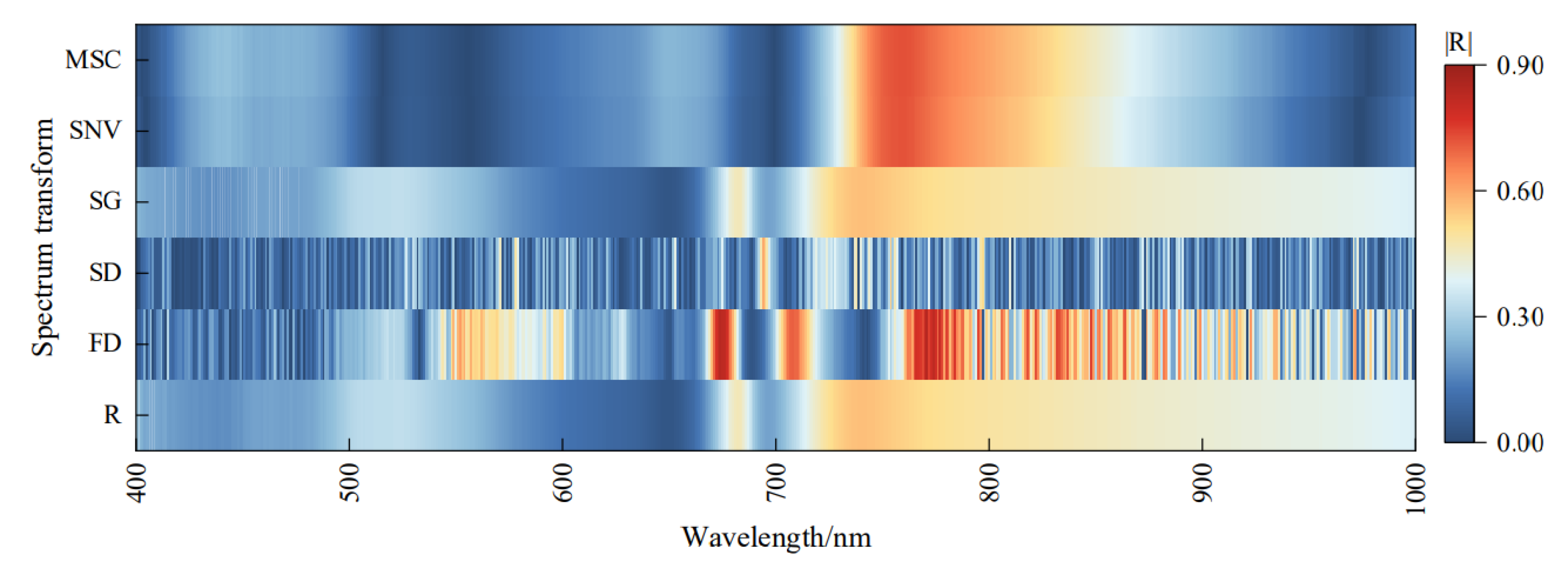
3.1. Spectral Data Transformation

Considering the influence of the instrument sampling interval, resolution, and noise, existing studies have shown that visible and near-infrared bands can reflect the physiological, biochemical and ecological status of plants [31]. This study finally selected the 400~1000 nm band, for a total of 601 bands for analysis. The original spectral reflectance of rice leaves and the spectral reflectance obtained through different spectral transformations are shown in Figure 2. From Figure 2a, it can be seen that the original spectral reflectance of rice leaves had the common characteristics of green plants. According to Figure 2b,c, the spectral shape after FD and SD transformation was completely different from the original spectrum, and the spectral features (absorption valley and reflection peak) were more prominent than the original spectrum. As shown in Figure 2d–f, the shape of the spectral curve after SG, MSC, and SNV transformation was still consistent with the original spectrum.
Since it is difficult to determine the influence and degree of spectral transformation on data based only on the change in spectral shape, correlation analysis of Fv/Fm with the original spectrum and the reflectance of the five transform spectra was first conducted. As shown in Figure 3, the correlation coefficients were higher in the range of 720–850 nm, and the maximum absolute value of the correlation coefficient (|R|) was 0.56, located at 740 nm. The correlation coefficients of the SG transformed spectrum were basically unchanged compared with the original spectra, and the maximum value of |R| and its corresponding wavelength both remained the same as the original spectra. After the SD transform spectrum, while some parts of the wavelengths’ correlation coefficients increased slightly (the maximum value of |R| was 0.60), overall, most of the correlation coefficients with the original spectrally sensitive wavelengths were reduced instead. Nevertheless, after the FD, MSC, and SNV spectra were transformed, the correlation between the spectral data and Fv/Fm significantly increased, the correlation coefficient-sensitive wave band was mostly concentrated in the 650~850 nm band range, and the maximum value of |R| reached 0.84, 0.73, and 0.72, respectively.
Then, the wavelength corresponding to the maximum absolute value of the correlation coefficient after each spectrum transformation was used to construct the linear, exponential, logarithmic, and quadratic polynomial equations with Fv/Fm, and the results are shown in Table 3. It can be seen from Table 3 that compared with the other three forms, the accuracy of the model constructed by FD, MSC, and SNV was improved to some extent, among which the quadratic polynomial equation constructed by the FD method had the best performance, with the R2, RMSE, and RPD of the testing set being 0.66, 2.66%, and 1.75, respectively, which reached the level of rough evaluation of Fv/Fm. The above results showed that FD, MSC, and SNV could mine the potential spectral feature information related to Fv/Fm, and simultaneously affect the accuracy of the model to a certain extent. Therefore, the three spectral transform methods were selected as the spectral pre-processing methods for the subsequent spectral feature extraction and model construction.

3.2. Spectral Feature Extraction Based on the CC and CARS Methods

Firstly, the CARS method was used to select the feature wavelengths of the full-spectrum data after FD, MSC and SNV spectral transformation. Taking MSC as an example, MCS times were set as 50, and the sampling times were iterated repeatedly. The selection process of the characteristic variables of the CARS algorithm is shown in Figure 4.
Figure 4a illustrates that with the continuous iteration of sampling times, the number of retained variables gradually decreased, and due to the effect of the EDF, the reduction speed of the number of variables decreased from fast to slow, indicating that there were two stages of “rough selection” and “fine selection” in the variable selection process of the CARS algorithm. Figure 4b shows that the RMSECV of the PLS model decreased first and then increased with increasing sampling times. In 1–25 iterations, RMSECV gradually decreased, indicating that information or noise unrelated to Fv/Fm in the spectral data was removed, while RMSECV gradually rose after 25 iterations, which showed that the important variables related to Fv/Fm in the spectral data were eliminated, and the information loss affected the performance of the model. The variation trend of the regression coefficients of all variables in each sampling process is shown in Figure 4c. According to Figure 4, the RMSECV value was the minimum when the number of runs was 25, that is, the selected subset of characteristic variables was optimal, which contained 37 characteristic variables, accounting for 6.16% of the total number of spectral variables. Table 4 shows that the characteristic bands screened by the CARS algorithm based on the spectral transformation of FD, MSC, and SNV accounted for 6.82%, 6.16%, and 4.33% of the total number of bands, respectively. The selected characteristic wavelengths were mainly located in the blue, red, and near-infrared regions.
However, the direct use of a variable selection algorithm to screen full-spectrum data easily causes low efficiency and information loss, while the combined use of different algorithms can take advantage of the complementarity between algorithms [32]. Therefore, the joint feature extraction method was used to extract the feature wavelength again. First, the sensitive wavelength whose correlation coefficient was in the top 1% based on the CC method was selected as the candidate feature wavelength subset, and then it was used as the input variable of the CARS method for the final spectral feature extraction, as shown in Table 4. As seen from Table 4, the characteristic bands screened by the CC-CARS algorithm based on the spectral transformation of FD, MSC, and SNV only accounted for 2.33%, 2.16%, and 2.66% of the total number of bands, which were reduced by 4.49%, 4%, and 1.67%, respectively, compared with the CARS method alone. At the same time, the selected feature wavelength was more concentrated in the red edge and near-infrared region.

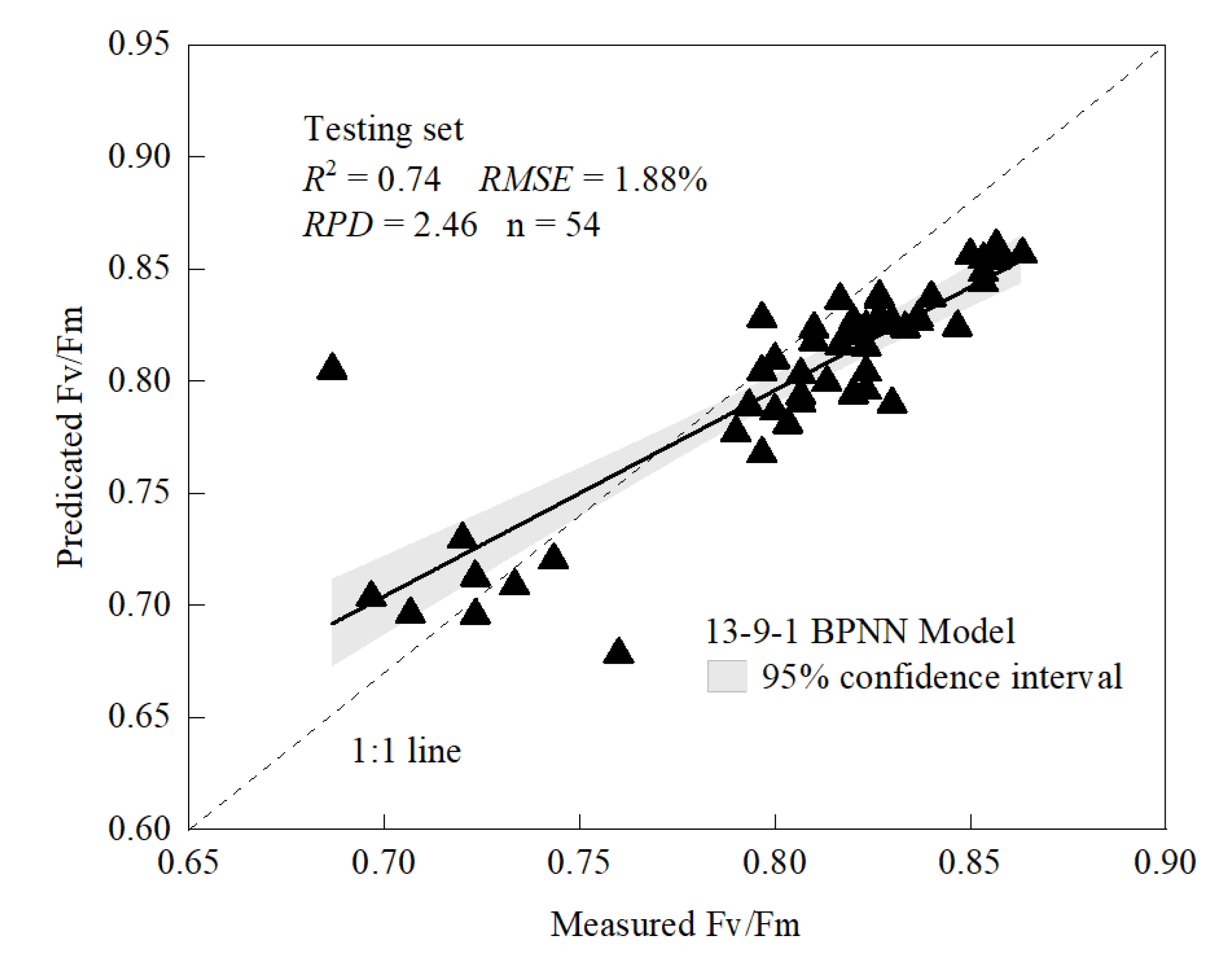
3.3. BPNN Model Construction and Accuracy Evaluation

Characteristic wavelengths screened by the CC, CARS, and CC-CARS algorithms were constructed as BPNN models and evaluated for model accuracy, and the results are shown in Table 5. Due to the strong nonlinear fitting ability of machine learning, the accuracy of the BPNN model based on the combination of different feature wavelengths was significantly improved. The R2 of the training sets all reached above 0.8, and the RPDs of the testing sets all reached the level of basic prediction evaluation of Fv/Fm. Among all the results, the characteristic wavelength optimized by MSC pre-treatment, and the CC-CARS algorithm was used as the input layer of the model, and the constructed 13-9-1 BPNN model had better robustness and generalization ability than the other models. Its testing set R2 was 0.74, RMSE was 1.88%, and RPD was 2.46, as shown in Figure 5.

4. Discussion

Spectral transformation can attenuate or eliminate spectral noise to varying degrees, extract weak spectral changes, and highlight useful spectral features, which has a great impact on the predictive performance of the model [33]. Although some studies have been conducted on the effects of different spectral transformation methods on the accuracy of monitoring Fv/Fm models [22,23], relatively few have been applied to monitor the rice leaf fluorescence parameters Fv/Fm. Based on this situation, the applicability of five spectral transformation methods (FD, SD, SG, MSC, and SNV) in the Fv/Fm monitoring of rice leaves was compared and analyzed in this study. The results of the correlation analysis and univariate model are shown in Figure 3 and Table 3. The data show that FD, MSC, and SNV transformations can more obviously highlight the correlation between spectral data and Fv/Fm, and it can be found that the sensitive bands with high correlation coefficients were mostly concentrated in the wavelength range of the chlorophyll fluorescence spectrum (650–800 nm) [34], consistent with the physiological basis of chlorophyll fluorescence. However, only a few methods commonly used in spectral data pre-processing were selected in this study. Therefore, in subsequent research, multiple spectral transformations, such as continuum removal [35], fractional differentiation [36], and continuous wavelet transform [18,19,26], should be used for comparison, and the combination of multiple spectral pre-treatment methods should also be tried.
The CC method can retain most of the objective and reasonable wavelength range to a certain extent and reduce the selection of characteristic variables. However, it is often difficult to determine a clear number of variables when completely relying on the CC method for selection. The CARS method can make maximum use of the existing sample set information to better analyze the combination effect among spectral variables [28]. The results of this study showed that the accuracy of the rice leaf Fv/Fm monitoring model constructed by using the characteristic wavelength selected by the CC-CARS method was better than that of the single CC method or CARS method (Table 5). Among them, the MSC-CC-CARS-BPNN model had the highest prediction accuracy, and the R2, RMSE and RPD of its testing set were 0.74, 1.88% and 2.46, respectively. Meanwhile, compared with the traditional vegetation index and independent feature extraction methods, the combined feature extraction method can improve the accuracy of the model to a certain extent [18]. This indicates that the combination of the CC method, which is a filtering method, and the CARS method, which is a packaging method, can make full use of the advantages of both, accurately select important feature wavelengths, reduce the difficulty of model learning, improve the prediction effect of the model, and enhance the generalization ability of the model [37].
Simultaneously, the characteristic wavelengths screened by the CC-CARS method accounted for only 2.16 to 2.66% of the full spectrum. In addition, compared to the CARS method alone, the wavelengths in the regions related to the absorption of photosynthetic pigments, such as plant chlorophyll a, chlorophyll b, and carotenoids, were more obviously excluded [23], and the characteristic wavelengths in the red and shortwave near-infrared regions were mainly retained. Since Fv/Fm is a key parameter of chlorophyll excitation fluorescence, the mechanism interpretation of keeping this part of the band as the characteristic wavelength of Fv/Fm parameter monitoring is relatively stronger. Existing studies have shown that there is a close relationship between chlorophyll excitation fluorescence and fluorescence of natural light [38,39]. Meanwhile, some scholars have carried out collaborative studies on the remote sensing of reflectivity and chlorophyll fluorescence [16,40,41], which indicates that passive remote sensing technology can be used to better assist the in-depth exploration of fluorescence active and passive joint observation in the future. However, this study only collected spectral reflectance at the leaf scale. If the study scale is extended to the canopy scale, the fluorescence signal will be affected by plant canopy structure, canopy heterogeneity, atmospheric action and other factors [18]. Therefore, multiscale comprehensive observations should be carried out in subsequent studies. To provide data and technical support for large-scale remote sensing monitoring of chlorophyll fluorescence parameters.
In this study, only the spectral monitoring of the chlorophyll fluorescence parameter Fv/Fm was evaluated. However, photochemical quenching (PQ) and non-photochemical quenching (NPQ), which are important components of the plant carbon fixation mechanism, will also affect the photosynthetic performance of plants [1], and there is a high degree of autocorrelation among massive fluorescence parameters [42]. Therefore, further comprehensive analysis and exploration should be carried out for the monitoring of other fluorescence parameters. At the same time, since this study was only conducted on rice, a large number of studies need to be carried out to verify the application of the research results on other plants. On the other hand, with the continuous development of machine learning, deep learning and other new technologies, there is a greater possibility for improving the accuracy and robustness of relevant monitoring models. Therefore, further exploration can be made on modelling methods in future studies to improve the accuracy of model prediction.

5. Conclusions

By comparison in this study, the BPNN model based on the characteristic wavelength extraction of MSC spectral pre-treatment and the CC-CARS method had the best monitoring effect on the Fv/Fm in rice leaves. Its testing set’s R2, RMSE, and RPD were 0.74, 1.88%, and 2.46, respectively. This study can provide a reference for the rapid non-destructive monitoring of chlorophyll fluorescence parameters by using spectral analysis technology.

Author Contributions

Conceptualization, J.L. and Z.G.; data curation, S.W., N.S. and Q.G.; formal analysis, S.W.; funding acquisition, Z.G.; investigation, S.W., N.S. and Q.G.; methodology, J.L.; project administration, Z.G.; resources, Q.G. and H.Y.; supervision, J.L.; validation, H.Y.; visualization, S.W.; writing—original draft, S.W.; writing—review and editing, J.L. All authors have read and agreed to the published version of the manuscript.

Funding

This study was funded by the National Key Research and Development Program of China (Gao Zhiqiang, 2018YFD0301006).

Institutional Review Board Statement

Not applicable.

Informed Consent Statement

Not applicable.

Data Availability Statement

Not applicable.

Conflicts of Interest

The authors declare no conflict of interest.

References

  1. Porcar-Castell, A.; Tyystjärvi, E.; Atherton, J.; van der Tol, C.; Flexas, J.; Pfündel, E.E.; Moreno, J.; Frankenberg, C.; Berry, J.A. Linking chlorophyll a fluorescence to photosynthesis for remote sensing applications: Mechanisms and challenges. J. Exp. Bot. 2014, 65, 4065–4095. [Google Scholar] [CrossRef] [PubMed] [Green Version]
  2. Tan, C.W.; Wang, D.L.; Zhou, J.; Du, Y.; Luo, M.; Zhang, Y.J.; Guo, W.S. Assessment of Fv/Fm absorbed by wheat canopies employing in situ hyperspectral vegetation indexes. Sci. Rep. 2018, 8, 9525. [Google Scholar] [CrossRef] [PubMed] [Green Version]
  3. Zheng, W.; Lu, X.; Li, Y.; Li, S.; Zhang, Y.Z. Hyperspectral identification of chlorophyll fluorescence parameters of Suaeda salsa in coastal wetlands. Remote Sens. 2021, 13, 2066. [Google Scholar] [CrossRef]
  4. Schreiber, U. Chlorophyll fluorescence as a tool in plant physiology I. The measuring systems. Photosynth. Res. 1983, 4, 361–373. [Google Scholar] [CrossRef] [PubMed]
  5. Bolhar-Nordenkampf, H.R.; Long, S.P.; Baker, N.R.; Oquist, G.; Schreiber, U.; Lechner, E.G. Chlorophyll fluorescence as a probe of the photosynthetic competence of leaves in the field: A review of current instrumentation. Funct. Ecol. 1989, 3, 497–514. [Google Scholar] [CrossRef]
  6. Kalaji, H.M.; Schansker, G.; Brestic, M.; Bussoyyi, F.; Calatyud, A.; Ferroni, L.; Goltsev, V.; Guidi, L.; Jajoo, A.; Li, P.; et al. Frequently asked questions about chlorophyll fluorescence, the sequel. Photosynth. Res. 2017, 132, 13–66, Erratum in Photosynth. Res. 2017, 132, 67–68. [Google Scholar] [CrossRef] [Green Version]
  7. Schreiber, U.; Bilger, W.; Neubauer, C. Chlorophyll fluorescence as a nonintrusive indicator for rapid assessment of in vivo photosynthesis. In Ecophysiology of Photosynthesis; Schulze, E.-D., Caldwell, M.M., Eds.; Springer: Berlin, Germany, 1995; pp. 49–70. [Google Scholar] [CrossRef]
  8. Ni, Z.Y.; Lu, Q.F.; Huo, H.Y.; Zhang, H.L. Estimation of chlorophyll fluorescence at different scales: A review. Sensors 2019, 19, 3000. [Google Scholar] [CrossRef] [Green Version]
  9. Yu, W.J.; Korner, O.; Schmidt, U. Crop photosynthetic performance monitoring based on a combined system of measured and modelled chloroplast electron transport rate in greenhouse tomato. Front. Plant Sci. 2020, 11, 1038. [Google Scholar] [CrossRef]
  10. Feng, W.; He, L.; Zhang, H.Y.; Guo, B.B.; Zhu, Y.J.; Wang, C.Y.; Guo, T.C. Assessment of plant nitrogen status using chlorophyll fluorescence parameters of the upper leaves in winter wheat. Eur. J. Agron. 2015, 64, 78–87. [Google Scholar] [CrossRef]
  11. Hazrati, S.; Sarvestani, Z.T.; Modarres-Sanavy, S.A.M.; Mokhtassi-Bidgoli, A.; Nicola, S. Effects of water stress and light intensity on chlorophyll fluorescence parameters and pigments of Aloe vera L. Plant Physiol. Biochem. 2016, 106, 141–148. [Google Scholar] [CrossRef]
  12. Cen, H.Y.; Yao, J.N.; Weng, H.Y.; Xu, H.X.; Zhu, Y.M.; He, Y. Applications of chlorophyll fluorescence in plant phenotyping: A review. Spectrosc. Spectr. Anal. 2018, 38, 3773–3779. [Google Scholar] [CrossRef]
  13. Zhao, R.M.; Xing, Z.Z.; Ma, X.Y.; Song, D.; Li, M.Z.; Sun, H. Correlation analysis and detection of photochemical absorption and reflectance spectra of potato leaves. Trans. Chin. Soc. Agric. Mac. 2020, 51, 375–381. [Google Scholar] [CrossRef]
  14. Xue, Z.C.; Gao, H.Y.; Peng, T.; Yao, G. Application of spectral reflectance on research of plant eco-physiology. Plant Physiol. J. 2011, 47, 313–320. [Google Scholar] [CrossRef]
  15. Butler, W.L.; Kitajima, M. Fluorescence quenching in photosystem II of chloroplasts. Biochim. Biophys. Acta 1975, 376, 116–125. [Google Scholar] [CrossRef]
  16. Hikosaka, K.; Tsujimoto, K. Linking remote sensing parameters to CO2 assimilation rates at a leaf scale. J. Plant Res. 2021, 134, 695–711. [Google Scholar] [CrossRef]
  17. Zhang, H.; Zhu, L.F.; Hu, H.; Zheng, K.F.; Jin, Q.Y. Monitoring leaf chlorophyll fluorescence with spectral reflectance in Rice (Oryza sativa L.). Procedia Eng. 2011, 15, 4403–4408. [Google Scholar] [CrossRef] [Green Version]
  18. Jia, M.; Li, D.; Colombo, R.; Wang, Y.; Wang, X.; Cheng, T.; Zhu, Y.; Yao, X.; Xu, C.; Ouer, G.; et al. Quantifying chlorophyll fluorescence parameters from hyperspectral reflectance at the leaf scale under various nitrogen treatment regimes in winter wheat. Remote Sens. 2019, 11, 2838. [Google Scholar] [CrossRef] [Green Version]
  19. Zhao, R.; An, L.; Song, D.; Li, M.; Qiao, L.; Liu, N.; Sun, H. Detection of chlorophyll fluorescence parameters of potato leaves based on continuous wavelet transform and spectral analysis. Spectrochim. Acta Pt. A Mol. Biomol. Spectrosc. 2021, 259, 119768. [Google Scholar] [CrossRef]
  20. Yang, Z.F.; Tian, J.C.; Feng, K.P.; Gong, X.; Liu, J.B. Application of a hyperspectral imaging system to quantify leaf-scale chlorophyll, nitrogen and chlorophyll fluorescence parameters in grapevine. Plant Physiol. Biochem. 2021, 166, 723–737. [Google Scholar] [CrossRef]
  21. Tan, C.W.; Huang, W.J.; Jin, X.L.; Wang, J.C.; Tong, L.; Wang, J.H.; Guo, W.S. Monitoring the chlorophyll fluorescence parameter Fv/Fm in compact corn based on different hyperspectral vegetation indices. Spectrosc. Spectr. Anal. 2012, 32, 1287–1291. [Google Scholar] [CrossRef]
  22. Li, B.; Gao, P.; Feng, P.; Chen, D.Y.; Zhang, H.H.; Hu, J. Prediction of eggplant leaf Fv/Fm based on Vis-NIR spectroscopy. Spectrosc. Spectr. Anal. 2020, 40, 2834–2839. [Google Scholar] [CrossRef]
  23. Wang, D.; Shen, K.C.; Fan, Y.M.; Long, B.W. Prediction method of chlorophyll fluorescence Fv/Fm image based on hyperspectral image. Trans. Chin. Soc. Agric. Mac. 2022, 53, 192–198. [Google Scholar] [CrossRef]
  24. Mohammadi-Moghaddam, T.; Razavi, S.M.A.; Taghizadeh, M.; Pradhan, B.; Sazgarnia, A.; Shaker-Ardekani, A. Hyperspectral imaging as an effective tool for prediction the moisture content and textural characteristics of roasted pistachio kernels. J. Food Measure. Characteriz. 2018, 12, 1493–1502. [Google Scholar] [CrossRef]
  25. Shen, L.Z.; Gao, M.F.; Yan, J.W.; Li, Z.L.; Leng, P.; Yang, Q.; Duan, S.B. Hyperspectral estimation of soil organic matter content using different spectral preprocessing techniques and PLSR method. Remote Sens. 2020, 12, 1206. [Google Scholar] [CrossRef] [Green Version]
  26. Wen, S.Y.; Shi, N.; Lu, J.W.; Gao, Q.W.; Hu, W.R.; Cao, Z.D.Y.; Lu, J.X.; Yang, H.B.; Gao, Z.Q. Continuous wavelet transform and back propagation neural network for condition monitoring chlorophyll fluorescence parameters Fv/Fm of rice leaves. Agriculture 2022, 12, 1197. [Google Scholar] [CrossRef]
  27. Cui, S.C.; Zhou, K.F.; Ding, R.F.; Zhao, J.; Du, X.S.H. Comparing the effects of different spectral transformations on the estimation of the copper content of Seriphidium terrae-Albae. J. Appl. Remote Sens. 2018, 12, 036003. [Google Scholar] [CrossRef]
  28. Jing, X.; Yan, J.M.; Zou, Q.; Li, B.Y.; Du, K.Q. Remote sensing monitoring of wheat stripe rust based on CC-MPA feature optimization algorithm. Trans. Chin. Soc. Agric. Mac. 2022, 53, 217–225+304. [Google Scholar] [CrossRef]
  29. Li, H.D.; Liang, Y.Z.; Xu, Q.S.; Cao, D.S. Key wavelengths screening using competitive adaptive reweighted sampling method for multivariate calibration. Anal. Chim. Acta 2009, 648, 77–84. [Google Scholar] [CrossRef]
  30. Zhang, Y.; Bai, L.C.; Qi, Y.; Huang, H.S.; Lu, X.Y.; Xiao, J.Q.; Lan, Y.B.; Lin, M.H.; Deng, J.Z. Detection of rice spikelet flowering for hybrid rice seed production using hyperspectral technique and machine learning. Agriculture 2022, 12, 755. [Google Scholar] [CrossRef]
  31. Peñuelas, J.; Filella, I. Visible and near-infrared reflectance techniques for diagnosing plant physiological status. Trends Plant Sci. 1998, 3, 151–156. [Google Scholar] [CrossRef]
  32. Song, X.Z.; Tang, G.; Zhang, L.D.; Xiong, Y.M.; Min, S.G. Research advance of variable selection algorithms in near infrared spectroscopy analysis. Spectrosc. Spectr. Anal. 2017, 37, 1048–1052. [Google Scholar] [CrossRef]
  33. Xiao, Q.L.; Tang, W.T.; Zhang, C.; Zhou, L.; Feng, L.; Shen, J.X.; Yan, T.Y.; Gao, R.; He, Y.; Wu, N. Spectral preprocessing combined with deep transfer learning to evaluate chlorophyll content in cotton leaves. Plant Phenom. 2022, 2022, 9813841. [Google Scholar] [CrossRef]
  34. Meroni, M.; Rossini, M.; Guanter, L.; Alonso, L.; Rascher, U.; Colombo, R.; Moreno, J. Remote sensing of solar-induced chlorophyll fluorescence: Review of methods and applications. Remote Sens. Environ. 2009, 113, 2037–2051. [Google Scholar] [CrossRef]
  35. Huang, Z.; Turner, B.J.; Dury, S.J.; Wallis, I.R.; Fole, W.J. Estimating foliage nitrogen concentration from HYMAP data using continuum removal analysis. Remote Sens. Environ. 2004, 93, 18–29. [Google Scholar] [CrossRef]
  36. Hong, Y.S.; Shen, R.L.; Cheng, H.; Chen, Y.Y.; Zhang, Y.; Liu, Y.L.; Zhou, M.; Yu, L.; Liu, Y.; Liu, Y.F. Estimating lead and zinc concentrations in peri-urban agricultural soils through reflectance spectroscopy: Effects of fractional-order derivative and random forest. Sci. Total Environ. 2019, 651, 1969–1982. [Google Scholar] [CrossRef]
  37. Feng, Z.H.; Li, X.; Duan, J.Z.; Gao, F.; He, L.; Yang, T.C.; Rong, Y.S.; Song, L.; Yin, F.; Feng, W. Hyperspectral remote sensing monitoring of wheat powdery mildew based on feature band selection and machine learning. Acta Agron. Sin. 2022, 48, 2300–2314. [Google Scholar] [CrossRef]
  38. Marrs, J.K.; Reblin, J.S.; Logan, B.A.; Allen, D.W.; Reinmann, A.B.; Bombard, D.M.; Tabachnik, D.; Hutyra, L.R. Solar-induced fluorescence does not track photosynthetic carbon assimilation following induced stomatal closure. Geophys. Res. Lett. 2020, 47, e2020GL087956. [Google Scholar] [CrossRef]
  39. Magney, T.S.; Frankenberg, C.; Fisher, J.B.; Sun, Y.; North, G.B.; Davis, T.S.; Kornfeld, A.; Siebke, K. Connecting active to passive fluorescence with photosynthesis: A method for evaluating remote sensing measurements of Chl fluorescence. New Phytol. 2017, 215, 1594–1608. [Google Scholar] [CrossRef] [Green Version]
  40. Kohzuma, K. Evaluation of photosynthetic behaviors by simultaneous measurements of leaf reflectance and chlorophyll fluorescence analyses. J. Vis. Exp. 2019, 150, e59838. [Google Scholar] [CrossRef]
  41. Tsujimoto, K.; Hikosaka, K. Estimating leaf photosynthesis of C3 plants grown under different environments from pigment index, photochemical reflectance index, and chlorophyll fluorescence. Photosynth. Res. 2021, 148, 33–46. [Google Scholar] [CrossRef]
  42. Ding, J.X.; Zhou, L.; Wang, Y.L.; Zhuang, J.; Chen, J.J.; Zhou, W.; Zhao, N.; Song, J.; Chi, Y.G. Application prospects for combining active and passive observations of chlorophyll fluorescence. Chin. J. Plant Ecol. 2021, 45, 105–118. [Google Scholar] [CrossRef]
Figure 1. Technology roadmap.
Agronomy 13 00337 g001
Figure 2. Different spectral data transformations.
Agronomy 13 00337 g002
Figure 3. |R| between Fv/Fm and spectral reflectance under different spectrum transforms.
Agronomy 13 00337 g003
Figure 4. Process of the CARS characteristic variable selection. (a) Variable retention rate; (b) change in RMSECV; (c) the trend of the variable regression coefficient.
Agronomy 13 00337 g004
Figure 5. The 1:1 relationship between the measured and predicted values of Fv/Fm.
Agronomy 13 00337 g005
Table 1. Fertilizer treatments in the experiment.
TreatmentsN1N2N3
Base fertilizer (kg/hm2)15–15–15 compound fertilizer300300300
lime600600600
Tillering fertilizer (kg/hm2)15–15–15 compound fertilizer3001500
urea22515075
Panicle fertilizer (kg/hm2)15–15–15 compound fertilizer757575
KCI454545
Table 2. Fv/Fm statistical characteristics of the different sample sets.
Sample SetSizeMax.Min.MeanCV (%)
All1620.860.660.815.54
Training set1080.860.660.815.64
Testing set540.860.690.815.34
Table 3. Performance of the Fv/Fm univariate model in the training and testing sets.
Spectrum TransformTraining SetTesting Set
RC2RMSEC (%)RV2RMSEV (%)RPD
Linear equationOR0.323.720.193.900.49
FD0.702.490.642.861.42
SD0.363.490.283.620.66
SG0.323.710.193.890.49
MSC0.533.240.473.101.03
SNV0.523.230.473.091.02
Exponential equationOR0.323.740.193.930.50
FD0.692.560.632.961.40
SD0.353.530.283.660.67
SG0.323.740.193.920.50
MSC0.523.300.463.171.05
SNV0.513.280.463.161.04
Logarithmic equationOR0.323.690.203.880.48
FD-----
SD0.373.450.283.600.68
SG0.323.680.203.870.48
MSC0.533.230.483.081.03
SNV0.533.210.483.051.03
Quadratic polynomial equationOR0.323.710.193.900.49
FD0.752.260.662.661.75
SD0.3711.40.2710.90.35
SG0.323.720.193.900.49
MSC0.582.950.552.681.12
SNV0.562.990.542.721.09
“-” indicates that part of the data is negative and cannot be calculated.
Table 4. Results of the CARS and CC-CARS characteristic variable selection.
Spectrum TransformNumber of VariablesWavelength Selection (nm)
CARSFD41463, 477, 482, 485–486, 495, 511, 513, 527, 529–530, 600, 642–643, 684, 699, 706–707, 750
762–763, 771, 775, 795, 851, 859, 863, 877–878, 912, 917, 944, 957, 965, 969, 983, 990–992, 994, 997
MSC37400, 404–406, 408–410, 412, 417–418, 421, 423, 427, 430, 436, 442–444, 452, 463, 499
554–555, 583, 659–661, 691–692, 704–705, 727, 907, 911, 930, 984, 998
SNV26403, 405, 408–410, 418, 421, 423, 430, 436, 442–444, 452–453
463, 671–672, 691–692, 702–703, 724, 911, 930, 998
CC-CARSFD14678–679, 707–710, 774–795, 832, 835 837, 864, 882, 889
MSC13742–743, 747, 753, 758, 773, 775, 785–786, 788, 794, 795, 800
SNV16744, 746, 749, 753, 767, 773, 775, 785–786, 788, 790, 794–797, 800
Table 5. Model construction and evaluation.
Spectrum TransformTraining SetTesting Set
RC2RMSEC (%)RV2RMSEV (%)RPD
CCFD0.901.440.692.071.92
MSC0.861.500.701.912.26
SNV0.831.870.692.101.94
CARSFD0.901.270.702.241.94
MSC0.841.770.682.471.83
SNV0.841.640.652.231.71
CC-CARSFD0.911.200.722.241.98
MSC0.861.500.741.882.46
SNV0.851.540.721.912.39
Disclaimer/Publisher’s Note: The statements, opinions and data contained in all publications are solely those of the individual author(s) and contributor(s) and not of MDPI and/or the editor(s). MDPI and/or the editor(s) disclaim responsibility for any injury to people or property resulting from any ideas, methods, instructions or products referred to in the content.

