Integration of Vis–NIR Spectroscopy and Machine Learning Techniques to Predict Eight Soil Parameters in Alpine Regions

Abstract

Visible and near-infrared spectroscopy (Vis–NIR, 350–1100 nm) has great potential for predicting soil properties. However, current research on the hyperspectral prediction of soil parameters in agricultural areas of alpine regions and the types of parameters included is limited, and optimal spectral treatments and predictive models applicable to different parameters have not been sufficiently investigated. Therefore, we evaluated the accuracy of predicting total nitrogen (TN), phosphorus pentoxide (TP₂O₅), total potassium oxide (TK₂O), alkali-hydrolyzable nitrogen (AHN), effective phosphorus (AP), effective potassium (AK), soil organic matter (SOM), and pH in the Qinghai–Tibet Plateau using the Vis–NIR technique in combination with spectral transformations, correlation analysis, feature selection, and machine learning. The results show that spectral transformations improve the correlation between spectra and parameters but are dependent on the parameter type and the method used. Continuum removal (CR), logarithmic first-order differential (FDL), and inverse first-order differential (FDR) had the most significant effects. The feature bands were extracted using the SPA and modeled using partial least squares (PLSR), random forest (RF), support vector machine (SVM), extreme gradient boosting (XGBoost), and backpropagation neural networks (BPNNs). The accuracy was evaluated based on R², RMSE, RPD, and RPIQ. We found that the PLSR model only enables the prediction of SOM and pH with lower accuracy than the remaining models. XGBoost can predict all of the parameters but only for AHN; the prediction performance is better than other methods (R² = 0.776, RMSE = 0.043 g/kg, and RPIQ = 2.88). The RF, SVM, and BPNN models cannot predict AK, AP, and AHN, respectively. In addition, TP₂O₅, AP, and pH are best suited for modeling using RF (RPIQ = 2.776, 3.011, and 3.198); TN, AK, and SOM are best suited for modeling using BPNN (RPIQ = 2.851, 2.394, and 3.085); and AHN and TK₂O are best suited for XGBoost and SVM, respectively (RPIQ = 2.880 and 3.217). Therefore, this study can provide technical and data support for the accurate and efficient acquisition of soil parameters in alpine agriculture.

1. Introduction

Soil is an important part of terrestrial ecosystems, and the cycles of its internal materials play an essential role in connecting the biosphere, atmosphere, and hydrosphere [1]. Changes in soil parameters have considerable impacts on soil quality [2] and directly affect the living environment of animals and plants, as well as the surrounding ecological conditions. This impact is more pronounced in ecologically fragile regions and areas sensitive to climate changes [3]. The Qinghai–Tibet Plateau, known as the “Roof of the World”, is an essential ecological security barrier and a vital water conservation area for China and even Asia [4]. It is also one of the major pastoral and forage-growing areas. The soil types on the Qinghai–Tibet Plateau are mainly alpine meadow soil and alpine steppe soil. The extensive alpine grasslands play a prominent role in mitigating global warming and are highly sensitive to global environmental changes [5,6,7]. In recent decades, the region has experienced a growing influence from climate change, human activities, engineering construction, and an escalation in rodent populations, resulting in significant issues such as alpine meadow degradation, land desertification, and soil erosion [8,9,10,11,12]. Research has indicated that a significant reduction in vegetation is the primary direct factor contributing to the degradation of the ecological environment on the Qinghai–Tibet Plateau. It also indirectly leads to reduced yields in agricultural production. The decline in vegetation results in soil degradation and animal migration [9,12]. Additionally, the soil environment is crucial for agriculture and animal husbandry. The physical and chemical properties of the soil, as well as the activity of microorganisms and enzymes, directly influence crop growth and animal survival. Diverse soil properties can directly indicate the soil’s fertility and quality, thereby serving as indicators for monitoring degradation. Therefore, the accurate, rapid, and nondestructive acquisition of soil properties is essential for precision agricultural and pastoral production, ecological monitoring, and management [13].

Total nitrogen (TN), total phosphorus pentoxide (TP₂O₅), total potassium oxide (TK₂O), alkali-hydrolysable nitrogen (AHN), available phosphorus (AP), available kalium (AK), soil organic matter (SOM), and pH value are essential parameters that reflect soil quality, and they are vital for the growth of crops [14,15,16]. For example, Sardans et al. [17] and Wu et al. [11] showed that C, N, and P are the major building blocks of soil nutrients and are essential for all biological processes and that vegetation growth and composition depend on the concentration of available nutrients in the soil. These parameters can be determined through laboratory chemical experiments. Although this method offers the advantage of high precision, it is burdened by the disadvantages of being time-consuming, potentially causing detrimental pollution, and leading to delayed outcomes [18]. Recently, continuously evolving visible and near-infrared technology (Vis–NIR) has gained extensive usage in classification and quantitative analyses owing to its advantages of high spectral resolution, strong wavelength continuity, and nondestructive nature [19]. Vis–NIR can reflect the overtones and combinations of basic molecular vibrations, such as clear responses to functional groups like C=O, N=H, and O=H. Many scholars have explored the prediction of soil parameters using Vis–NIR technology and achieved good results [20,21,22], for instance, the physical and chemical properties of soil and the composition of minerals, including TN [23], SOM [14], soil moisture [24], organic carbon [25], soil exchangeable cations [26], and the soil adsorption coefficient of glyphosate [27]. However, there are differences in Vis–NIR prediction models in different regions due to regional differences in soil types and physicochemical properties, surface cover, and climate. Prediction of the same soil parameter may involve different treatments and models, leading to differences in prediction accuracy [28]. For example, Conforti et al. found that soil grain size, sand content, and phyllosilicates can significantly change the soil spectral shape and greatly impact the estimation of soil properties. EI-Sayed et al. [29] used Vis–NIR to estimate the pH and salinity in arid agricultural areas of Egypt and found PLSR’s to be the optimal model, while Wang [30] et al. found that the limit learning machine performed the best in the study of lime-cured black soil. Similarly, there are often differences in preprocessing and modeling methods for the hyperspectral prediction of the same parameters (SOM [31,32], TN [33,34], and quick nutrients [34,35]) due to differences in soil properties, environments, etc. In addition, because of the extremely high spectral resolution of hyperspectral data, the acquired data often suffer from covariance, spectral band overlap, and interactions [36,37]. Full-band modeling typically includes a lot of data that do not contain critical information, which increases the model complexity while degrading the model performance [36,38]. It is therefore necessary to perform dimensionality reduction or feature selection on hyperspectral data in order to remove uninformative variables and reduce the model complexity. In chemometric analysis studies of NIR spectra, the commonly used feature selection methods are the successive projection algorithm (SPA), uninformative variable elimination (UVE), competitive adaptive reweighted sampling (CARS), and recursive feature elimination (RFE). Among them, SPA can extract the variables with the least amount of redundant information from the spectral data, maximize the covariance reduction problem, and is one of the most commonly used feature extraction methods in the chemometric analysis of soil spectra [36,37,38,39].

Currently, research on predicting soil parameters using Vis–NIR technology is mainly focused on plains agricultural areas, forested areas [35], black soil regions [40,41], mining areas [42], and wetlands [43]. For instance, Kawamura et al. [35,44] used Vis–NIR technology, machine learning, and deep learning methods to predict the total carbon and phosphorus content in the soils of rice paddies and forested areas in Madagascar. Pudełko et al. [42] used hyperspectral imaging technology and Fourier-transform near-infrared spectroscopy combined with machine learning techniques to predict soil nitrogen and organic carbon content in mining areas. They found that hyperspectral imaging could predict organic carbon content more accurately, but its accuracy in predicting nitrogen content was similar to other methods. Similarly, Peng et al. [45] employed Vis–NIR combined with PLSR, BPNN, and GA-BPNN methods to predict TP, TN, and TK in cultivated soils, and they found that GA-BPNN and BPNN performed better than PLSR in predicting soil nutrients, and GA-BPNN was the best. Meanwhile, predictive studies have been carried out for the organic matter, TS, TK, and heavy metal content of soils in these areas, and the R² values of the predictive models ranged from 0.6 to 0.95 [46,47]. However, different modeling methods and parameters have different accuracies. In general, the modeling accuracy is deep learning models > machine learning models > linear models but may vary depending on the parameters or region [27,48,49]. Deep learning often requires a large amount of training data to improve the accuracy and robustness of the model, and a small amount of data suffers from many problems, such as difficulty in convergence and overfitting. Therefore, machine learning is the main method used in prediction studies and performs well with small samples [50,51]. Kawamura et al. [35,44] found that the machine learning model showed higher accuracy than the traditional linear model (e.g., multiple linear stepwise regression and partial least squares) when predicting soil parameters (e.g., N and P) using Vis–NIR. Previous research in their study on predicting soil TN using Vis–NIR technology combined with support vector machines, random forests, extreme gradient boosting (XGBoost), and backpropagation neural networks discovered that all machine learning methods could achieve accurate TN predictions, with the model accuracy ranking as follows: RF > BPNN > SVM [37,45,52,53]. XGBoost’s performance may be higher or somewhere in between. Therefore, it can be observed that machine learning methods are better at utilizing spectral information to predict soil properties. Most of the above research did not involve studies in alpine agricultural areas and involved a few types of soil parameters. In addition, in terms of modeling methods, most of them used only one or a few spectral transforms and machine learning methods without a general comparative analysis and the optimal treatment and modeling methods for different soil parameters in alpine agricultural areas are not given.

Therefore, this paper aimed to conduct a prediction study of TN, TP₂O₅, TK₂O, AHN, AP, AK, SOM, and pH contents in agricultural soils (pasture-growing areas) on the Tibetan Plateau using visible-near-infrared (Vis–NIR) technology to establish the optimal spectral prediction model for eight parameters. Meanwhile, the optimal spectral processing and modeling methods for the prediction of eight soil parameters in alpine agricultural areas are further clarified. Finally, an optimal hyperspectral prediction model for eight parameters of alpine agricultural soils is developed, and the optimal spectral treatments for different parameters is determined.

2. Materials and Methods

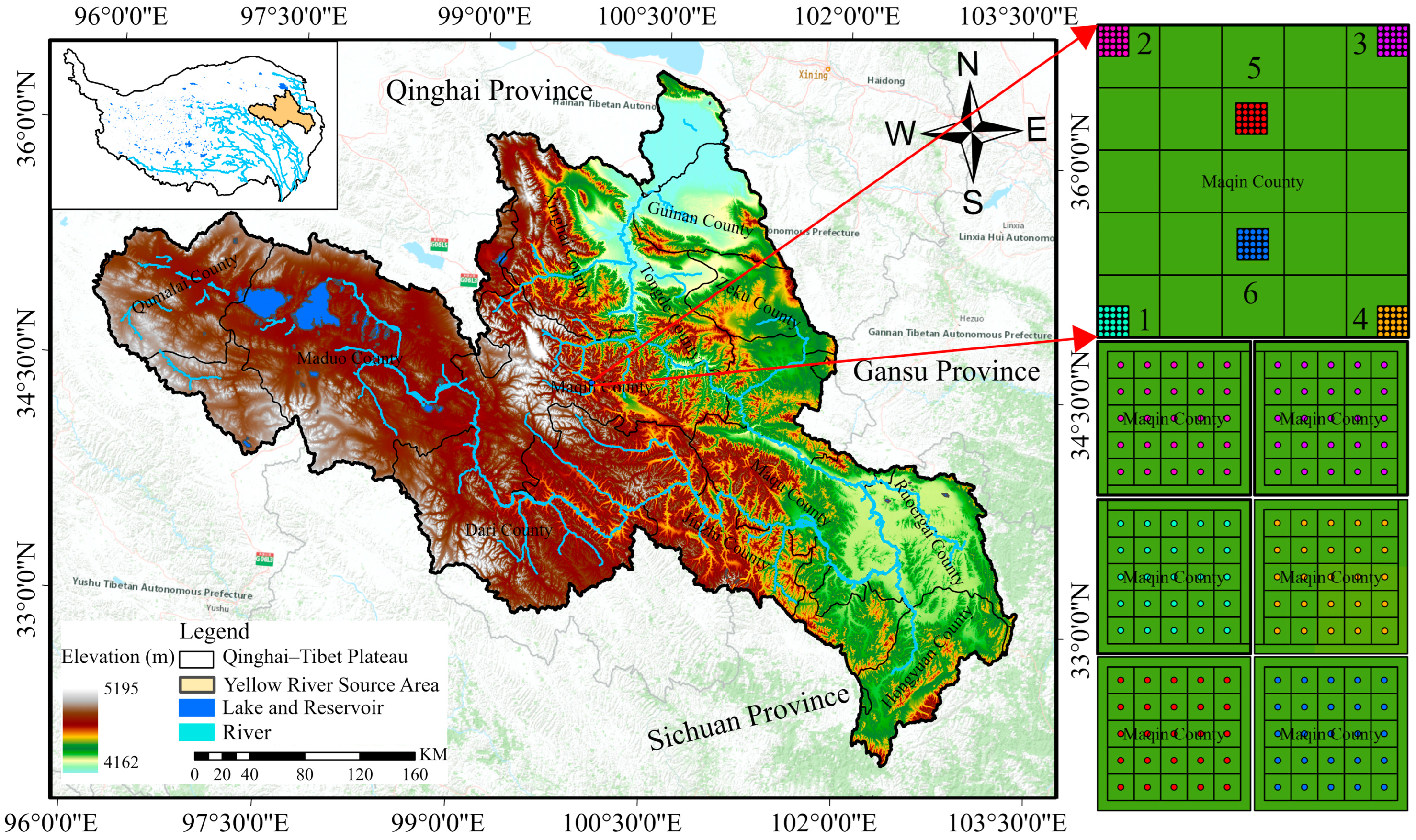
2.1. Study Area and Soil Sample Collection

The source area of the Yellow River is located in the northeast of the Tibetan Plateau (32°12′ N–36°36′ N, 95°54′ E–103°24′ E), which involves Qinghai, Gansu, and Sichuan provinces, with a total area of 13.2 × 104 km², and accounts for approximately 16% of the total area of Yellow River Basin [5,54,55]. The elevation of the study area ranges from 2457 m to 6254 m and experiences sub-cold semi-arid and semi-humid climate, with no clearly defined seasons. The annual average temperature is approximately 0.0 °C, with the average temperature of the coldest month reaching –10.6 °C and the annual average precipitation ranges between 300 mm and 700 mm [56]. The vegetation types are rich and widely distributed. Alpine meadows, alpine grassland, and alpine shrubs account for about 75% of the total area, with alpine meadows taking up the largest proportion [57]. The sampling area was located in the pasture-growing area of Dawu town, Maqin county, in the middle of the source region of the Yellow River. This region is characterized by shallow soil thickness, coarse soil texture, and limited water retention [58]. Figure 1 shows the location of the six sampling plots and the elevation of the study area.

Soil samples were obtained from the Yellow River source area in July 2023 and August 2023, with the sampling points covering the original alpine meadow, restoration area, and degradation area (Figure 1). A 200 × 200 m sample plot was set up in the central area of the Yellow River source, and then a 20 × 20 m sample square was set up at each of the four corners and the center of the sample plot. Subsequently, the sample square was evenly divided into 5 × 5 squares, and soil samples were collected in the center of each square. We established the soil sampling depth at 5–10 cm, considering that the root system of alpine meadow vegetation is primarily concentrated in the surface layer of 0–20 cm, thereby minimizing the damage to the alpine meadow [59,60,61]. Soil samples were collected using a cutting ring at a depth of 5–10 cm in the surface soil, and interference objects such as weeds were removed. One hundred and fifty soil samples were collected.

2.2. Data Collection and Processing

The soil samples collected were placed in an aluminum box and subjected to baking in a constant temperature oven at 105 ± 2 °C for 12 h. After baking, they were removed, covered, and transferred to a desiccator to cool to room temperature (for 30 min). The dried soil samples were ground (through a 2 mm sieve) using a grinder. Each soil sample was divided into two equal parts: one measurement of its AHN, AK, AP, SOM, TN, TK₂O, TP₂O₅, and pH values, and the other was used for soil spectral reflectance measurements. The PSR-1100F (AZUP Scientific Co., Limited, Beijing, China) portable ground-object spectrometer with a range of 320–1100 nm and a spectral interval of 1 nm (resolution = 3 nm) was used to measure the spectral reflectance; the light source was a 50 W halogen lamp, the light source zenith angle was 45°, and the optical fiber probe was about 5 cm away from the sample. The instrument was preheated for 30 min before measurement, and then the whiteboard was measured for instrument calibration. The soil samples were loaded into glass Petri dishes and flattened on the surface, followed by data collection using a PSR-1100F spectrometer. The spectral data were collected at six different locations on the surface of each soil sample. Each sample was repeated three times, and the average value was taken as the final result. The instrument must be calibrated with a whiteboard before measuring each sample. The collected spectral data require preprocessing because the measured data have some noise from the instrument’s factors and external environment interference. Firstly, the spectral data were smoothed with Savitzky–Golay (S–G) filtering (first derivative filter: bandwidth = 5; polynomial fitting order = 2). In addition, because of the instrument itself, the edge band of the low signal-to-noise ratio (320–399 nm) was removed before filtering. The contents of TN, SOM, TP₂O₅, AHN, AP, and TK₂O of the soil samples were measured using the semi-micro Kjeldahl method; the external heating with potassium dichromate method; the molybdate colorimetric method after the perchloric acid digestion; and the alkalotic-diffusion method, sodium hydrogen carbonate solution-Mo-Sb anti spectrophotometric method, and the flame photometry method after melting with sodium hydroxide [62]. The content of AK was obtained by leaching the soil with NH₄OAc, and the soil leaching solution was obtained and then measured directly with the flame photometer. The pH values of the soil samples were measured using the potentiometry method.

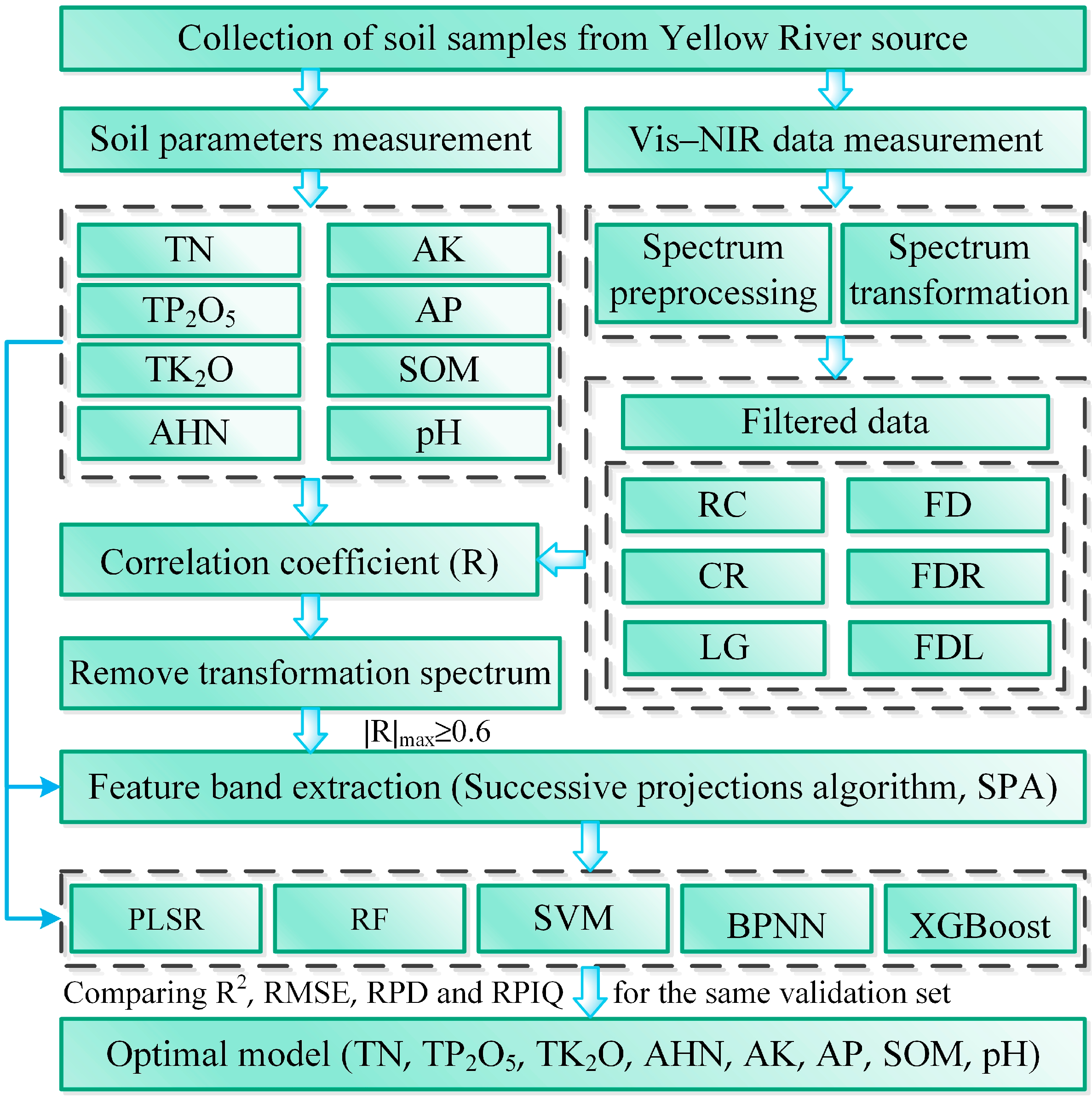
2.3. Research Methodology and Development of Models

Soil samples and hyperspectral data from the sample plot were collected during fieldwork. The spectral reflectance (R) was subjected to Savitzky–Golay (S–G) smoothing and reciprocal (RC), logarithmic (LG), continuum removal (CR), first derivative (FD), first derivative of reciprocal (FDR), and first derivative of logarithmic (FDL) transformations. The correlation coefficient between the transformed spectral data and soil parameters was calculated. The level of correlation between the spectral data and soil parameters can reflect the response characteristics of each band to soil parameters. It can be used to extract the feature bands of the spectrum. Therefore, we removed the transformed spectra whose maximum absolute value was less than 0.6 to construct a high-performance model more effectively and reduce unnecessary data processing. Then, the feature bands of the remaining spectra were screened using the successive projection algorithm (SPA). Modeling was performed using partial least squares (PLS), random forests (RFs), support vector machines (SVMs), Extreme gradient boosting (XGBoost), and back propagation neural networks (BPNNs). The model hyperparameters were searched using random grid optimization, and the mean values of R², RMSE, RPIQ, and RPD of the model were calculated with 5-fold cross-validation. The validation sample verified the established model’s accuracy. Figure 2 shows the technical roadmap for the present work.

2.3.1. Pearson Correlation

The effect of the transformation methods was analyzed by calculating the Pearson correlation coefficients between different transformation spectra and soil parameters, and the threshold value of the correlation coefficient was set to decide whether a certain transformation method could be used in the subsequent prediction model. The Pearson correlation coefficient was calculated using Equation (1) [28].

$$r_i=\frac{{\displaystyle \sum _{n=1}^N(X_{ni}-{\overline{X}}_i)(Y_n-\overline{Y})}}{\sqrt{{\displaystyle \sum _{n=1}^N{(X_{ni}-{\overline{X}}_i)}^2{\displaystyle \sum _{n=1}^N{(Y_n-\overline{Y})}^2}}}}$$

(1)

where $r_i$ is the correlation coefficient between the soil parameter $Y$ and spectral reflectance $X$, $i$ is the band number, $X_n$ is the spectral reflectance of the $n$-th soil sample in the $i$ band, ${\overline{X}}_i$ is the mean value of the $N$ spectral reflectance in the i band, $Y_n$ is the soil parameters of the $n$-th soil sample, $\overline{Y}$ is the mean value of the $N$ soil sample parameters, and $N$ is the number of samples.

2.3.2. Feature Selection Algorithm

Hyperspectral data have a very high spectral resolution, enabling them to capture abundant information about the target object. However, an excessive spectral resolution can lead to strong correlations between adjacent bands, resulting in information redundancy and, consequently, unstable convergence of multivariate prediction models. Therefore, using fewer bands can build more stable models and make it easier to carry out subsequent analysis and processing [63].

The successive projection algorithm (SPA) is a technique for reducing dimensionality based on variable information. It employs vector projection analysis to identify variable combinations that carry minimal redundant information. The SPA can efficiently alleviate collinearity, singularity, and spectral band instability, leading to the reduction of collinearity among vectors and a decrease in the number of variables used in modeling. This reduction in variables contributes to the reduction of model complexity [64]. Its fundamental principle is as follows [65]:

First, define the spectral matrix as X_n×m (n is the number of samples, and m is the number of spectral variables); then, set the number of variables to be selected, H, and perform the following steps:

• Let t₀ = 1, choose any column vector in X_n×m as x_k(0), k(0) is the initial position of the selected variable x (j = k(0), 1 ≤ j ≤ m), the set of other remaining variable positions is defined as s:

  $$s=\left\{j,1\le j\le m,j\notin \left\{k(0),\cdots ,k(H-1)\right\}\right\}$$

  (2)
• Compute the projection of the remaining column vector x_j$(j\in s)$ onto the orthogonal vector space formed by the selected vector x_k(t−1):

  $$P=I-\frac{x_{k(t-1)}{(x_{k(t-1)})}^T}{{(x_{k(t-1)})}^T{x}_{k(t-1)}}$$

  (3)

  $$x_j=P{x}_j$$

  (4)

  where I is the unit matrix, and P is the projection operator;
• Select the maximum projection value variable $\arg \left[\max \left(‖P{x}_i‖\right)\right],j\in s$ to add to the set of selected variables;
• Let t = t + 1, if t < H, then return to step (2) for circular calculation.

When the loop ends, the set $\left\{x_{k\left(0\right)},x_{k\left(1\right)},\cdots ,x_{k\left(H\right)}\right\}$ of selection variables is obtained. Because x_k(0) is randomly selected, each column in the spectral matrix needs to be iterated as x_k(0) to obtain n candidate vector sets $X={\left\{X_1,X_2,\cdots ,X_n\right\}}^T$ containing H variables. Then PLS is used to cross-validate each variable set in X. The corresponding variable combination with the smallest root mean square error of cross-validation (RMSECV) is selected, and the final selection of feature bands is obtained

2.3.3. Regression Model

All samples were randomly divided into training and validation sets in the ratio of 8:2, 120 training samples 30 independent validation samples (split using train_test_split in Sklearn 1.3.0 library). In addition, to improve the performance of the PLSR, RF, SVM, and BPNN models, as well as to assess the accuracy of the model predictions, we performed nested 5-fold cross-validation in the training set to optimize the hyperparameters and to assess the performance of the models. The outer loop of the cross-validation was used for testing the model performance, while the inner loop was utilized to optimize the hyperparameters of PLSR, SVM, RF, and BPNN. For the BPNN, we employed one of the internal folds to determine when to halt the training process.

• PLSR model

PLSR is a linear regression model constructed by projecting predictor and observable variables onto a new space. It is well suited for analyzing high-dimensional datasets (e.g., hyperspectral data and Vis–NIR data) and is a widely used linear regression method. PLSR combines information from all available bands without the problem of multicollinearity. PLSR treats each band as an independent explanatory variable that is used to estimate the response variable for the target component (soil parameter in this study). Here, a randomized grid search (5-fold cross-validation) was used to determine the optimal number of PLS factors to include in the model.

2.

RF model

Random forest (RF), proposed by Breiman et al. [66], is an integrated learning algorithm that uses multiple decision trees to solve classification and regression problems and is part of an integrated learning algorithm in which there is no dependency between weak learners. Its advantage is reflected in parallelized operation, so there is little correlation between randomly selected decision trees, improving the model’s accuracy [67]. It also has obvious advantages in terms of parameter optimization, variable ranking, and subsequent variable analysis and interpretation and is able to make full use of sample data [68].

For the random forest (RF) model, three hyperparameters were optimized: number of decision trees (n_estimators), maximum depth (max_depth), and minimum number of samples per leaf (min_samples_leaf). The parameter n_estimators was explored across 50 evenly spaced values between 50 and 500; max_depth was examined with 50 values ranging from 10 to 500; min_samples_leaf was searched among the values 1, 2, 3, and 8.

3.

SVM model

Support vector machine (SVM) is a machine learning algorithm based on statistical learning theory, which takes statistical learning theory as its system and pursues optimal results under the condition of limited information by seeking to minimize structural risk and has the advantage of applying to high-dimensional feature spaces, small sample statistical learning, and strong resistance to noise influence in data processing [69,70,71]. It has the advantages of being suitable for high-dimensional feature space, small sample statistical learning, and resistance to noise. Soil spectra are affected by many factors such as organic matter and moisture, which is a complex process, and the number of samples is limited, so the study chose a more suitable support vector machine model for prediction. The key to SVM modeling is the selection of the parameters (penalty cost and radius of kernel function gamma) and the kernel function. Cost and gamma are obtained by cross-validation, and the widely used radial basis (RBF) function is selected as the kernel function based on the obtained cost and gamma.

The support vector machine (SVM) model employed the radial basis function (RBF) as its kernel, and the penalty parameters C, gamma, and epsilon were searched across 50 increasing values from 1 × 10⁻⁵ to 100.

4.

BPNN model

The BPNN consists of input, hidden, and output layers and is learned using an error back propagation algorithm. The BPNN model error is back propagated to the hidden layer each time and, subsequently, back propagated to the input layer at each iteration. Then, the weights connecting the input neurons (processing elements in the neural network) and the hidden neurons are randomly varied to establish a better correlation between the input neurons and the actual outputs, which is suitable for analyzing a variety of nonlinear relationships. In this study, the input layer is the spectral data of the soil, and the output layer is the data of each soil parameter [47].

For the backpropagation neural network (BPNN), optimization was carried out using the stochastic gradient descent (SGD) optimizer. Activation functions were explored among “logistic”, “tanh”, and “relu”. Learning rates were searched within the values of 0.0001, 0.0005, 0.001, 0.005, 0.01, and 0.1. The number of hidden layers was 3, and the number of neurons in each layer was searched among 16, 32, 64, 128, and 256.

5.

XGBoost model

Extreme gradient boosting (XGBoost) is a scalable end-to-end tree enhancement algorithm [72]. XGBoost not only utilizes the first-order derivatives of the loss function but also performs a second-order Taylor expansion of the loss function by taking into account the second-order derivative information. This study uses the root mean square error (RMSE) as the loss function to evaluate the optimal objective function [37]. The model’s generalization ability, as well as the prevention of overfitting, is improved by incorporating regularization.

The hyperparameters of the XGBoost model were tuned as follows: the maximum depth of the tree was searched in 3, 5, 7, and 9; the learning rate was searched in 0.01, 0.015, 0.025, 0.05, 0.1, and 0.2; and the gamma was searched in 0, 0.05, 0.1, 0.3, and 0.5.

All models and optimization algorithms were implemented using the “sklearn 1.3.0” and “keras 2.8.0” libraries [73,74].

2.3.4. Evaluation of Model Accuracy

The model was applied to the validation sets, and the accuracy of the hyperspectral inversion models of the soil parameters was measured using the determination coefficient (R²), root mean square error (RMSE), residual prediction deviation (RPD), and performance to interquartile distance (RPIQ) (5-fold cross-validation). The calculation method was as follows [35,75]:

$$R^2=1-\frac{{\displaystyle \sum _{i=1}^n{\left(y_i-Y_i\right)}^2}}{{\displaystyle \sum _{i=1}^n{\left(y_i-{\overline{y}}_i\right)}^2}}$$

(5)

$$RMSE=\sqrt{\frac{1}{n}{\displaystyle \sum _{i=1}^n{(Y_i-y_i)}^2}}$$

(6)

$$RPD=\frac{SD}{RMSE}=\sqrt{\frac{\raisebox{1ex}{$1$}\!\left/ \!\raisebox{-1ex}{$n-1$}\right.{\displaystyle \sum _{i=1}^n{(y_i-\overline{y})}^2}}{\raisebox{1ex}{$1$}\!\left/ \!\raisebox{-1ex}{$n$}\right.{\displaystyle \sum _{i=1}^n{(Y_i-y_i)}^2}}}$$

(7)

$$RPIQ=\frac{Q_3-Q_1}{RMSE}$$

(8)

where $Y_i$ is the predicted value, $y_i$ is the observed value, $\overline{y}$ is the average value of $y_i$, and n is the sample number; Q₁ and Q₃ are the values below which we can find 25% and 75% of the samples (in ascending order). A larger $R^2$ and a smaller $RMSE$ indicates a better fitting effect of the model; an $RPD$ greater than 1.4 indicates good prediction capacity, and a value larger than 2 suggests excellent prediction performance [46]; RPIQ is unitless and based on quartiles, and the bigger the value, the better.

3. Results and Analysis

3.1. Soil Parameters and Spectrum Feature Analysis

The statistical results of the measurements for various soil parameters are shown in

Table 1. Statistical results of the parameters of the soil samples.

Soil Parameters	Minimum Value (g/kg)	Maximum Value (g/kg)	Mean Value (g/kg)	Standard Deviation (g/kg)	Coefficient of Variation
TN	0.450	4.510	2.372	0.942	0.397
TP2O5	1.020	5.920	1.539	0.815	0.529
TK2O	13.790	22.480	19.225	1.956	0.101
AHN	0.045	0.317	0.183	0.076	0.415
AP	0.003	0.050	0.008	0.007	0.918
AK	0.040	0.360	0.162	0.071	0.441
SOM	4.070	92.190	41.660	20.443	0.490
pH	6.300	9.060	7.794	0.714	0.091

Note that pH has no units in the table.

. Table 1 shows that the soil SOM and TK₂O contents in the alpine agricultural area where the sample was located were more than the other parameters, with maximum values of 92.190 and 22.480, respectively. The content of efficient nutrients was the lowest. The coefficient of variation shows that the fluctuation of the AP content was the largest, followed by TP₂O₅, SOM, and AK, indicating that the AP content varied the most among different sampling sites.

After S–G filtering of the original soil spectral reflectance data, RC, CR, LG, FD, FDR, and FDL transformations were performed, as shown in Figure 3. It was found that the reflectance of each soil sample ranged from 0 to 100%, the spectral curve of each sample was similar to each other after S–G filtering, the overall trend was gentle, and the reflectivity decreased first (400–420 nm) and then increased (420–1100 nm); the various spectral transformations, especially the CR and FDL transformations, considerably amplified the original spectral characteristics.

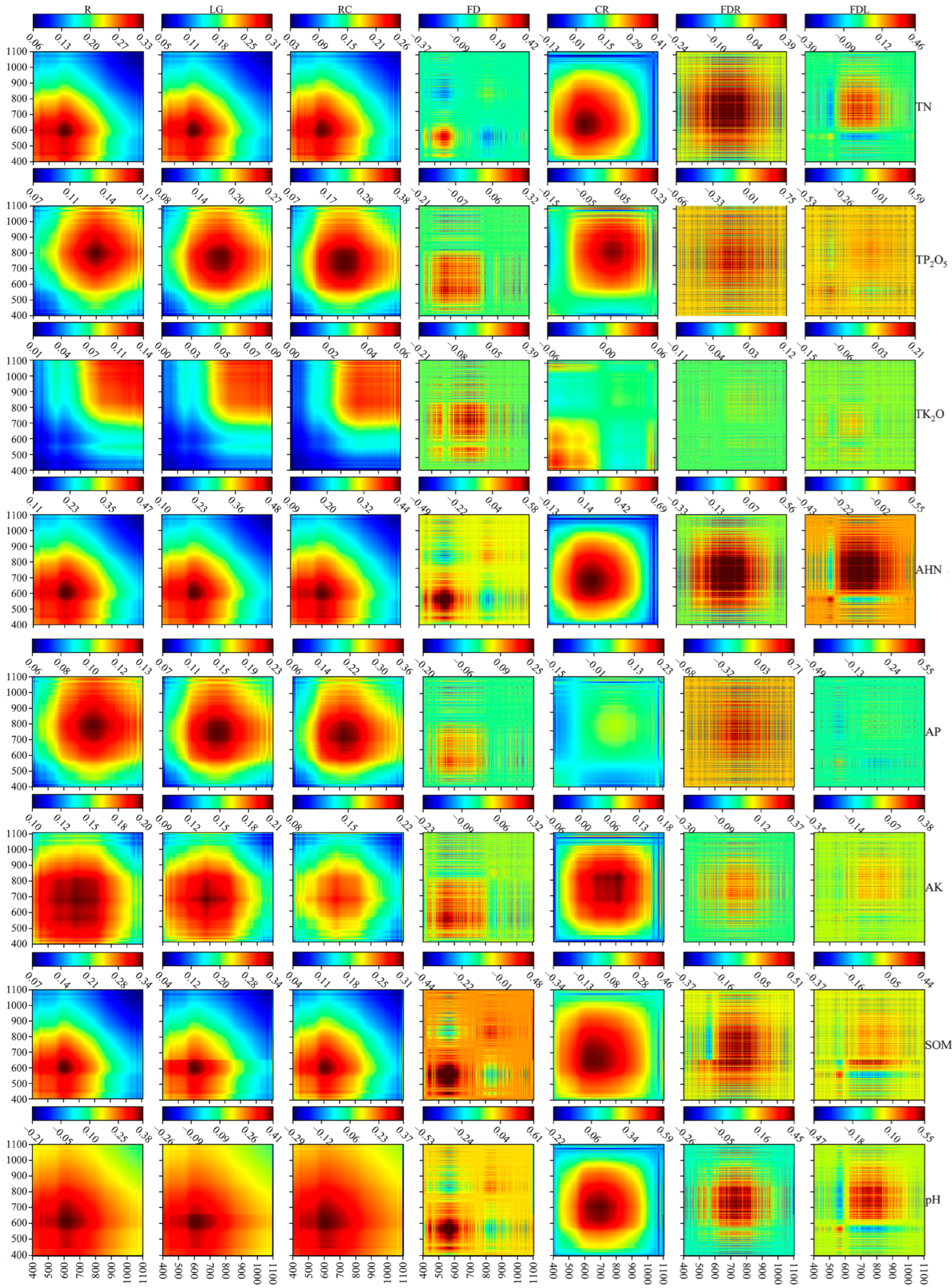
3.2. Correlation Analysis

The correlation coefficients were calculated for each of the eight soil parameters with seven forms of spectra (Equation (1)), and a total of 150 correlation coefficient vectors of size (701 × 1) were obtained r_i (i = 1, 2, …, 150). The maximum absolute correlation coefficients of each parameter with the corresponding spectrum are presented in

Table 2. Maximum absolute values of correlation coefficients between soil parameters and spectra.

Soil Parameters	Spectral Transformation Type
	S–G	RC	LG	CR	FD	FDR	FDL
TN	−0.58 **	0.51 **	−0.56 **	−0.64 **	−0.65 **	−0.62 **	0.68 **
TP2O5	−0.42 **	0.62 *	−0.52 *	−0.48	−0.57	−0.86 *	−0.77
TK2O	−0.37	0.24	−0.30	−0.25	−0.620 *	0.35	−0.46
AHN	−0.68 **	0.66 **	−0.69 **	−0.83 **	−0.76 **	−0.75 **	0.74 **
AP	−0.37 **	0.60 *	−0.48 *	−0.47	−0.50	−0.84 *	−0.75 *
AK	−0.45 **	0.45 **	−0.45 *	−0.42 **	−0.57 **	−0.60 **	0.61 **
SOM	−0.58 **	0.56 **	−0.58 **	−0.68 **	−0.69 **	−0.68 **	0.72 **
pH	0.62 **	−0.61 **	0.63 **	0.77 **	0.78 **	0.67 **	−0.74 **

*, ** Significantly correlated at the 0.05 and 0.01 levels (bilateral), respectively.

. From Table 2, it is evident that the correlation coefficients for AP and TP₂O₅, utilizing the FDR-transformed spectral data, and that of TK₂O with the FD-transformed spectral data, witnessed the most significant improvements, which increased by 168.4%, 207.7%, and 230.0%, respectively. TN, AK, and SOM had the highest correlation coefficients, with FDL-transformed spectra being 0.68, 0.61, and −0.74, respectively. AHN demonstrated the highest correlation coefficient, notably −0.83 after CR transformation. pH had the highest correlation coefficient, with FD-transformed spectra being 0.78. However, some transformations reduced the correlation of spectra with soil parameters, such as TN with RC and LG, TK₂O with RC, LG, CR, and FDR. Therefore, although the mathematical transformation of soil spectral data can effectively improve its correlation with soil parameters, the transformation methods need to be selected, and the best transformation methods are different for different soil parameters.

In addition, the one-dimensional correlation coefficients were visualized in two dimensions to facilitate the analysis of the correlation between the spectral reflectance and soil parameters at different wavelengths. That is, $r_i^{\prime }=r_i\times r_i^T$, where $r_i^{\prime }$ is the matrix of the correlation coefficients after two-dimensionalization with a size of 701 × 701. The results are shown in Figure 4.

Figure 4 shows that the LG and RC transformations did not change the sensitive bands of the soil spectrum, and the high values of the correlation coefficients were relatively concentrated. The high values of the correlation coefficients of TN, AHN, SOM, and pH with the S–G, LG, and RC spectra were concentrated in the range of 400–800 nm; the high values of the correlation coefficients of TP₂O₅ and AP with the S–G, LG, and RC spectra were concentrated in the range of 600–1000 nm, while AK was in the range of 400–900 nm. In addition, the high-value region of the correlation coefficients of TK₂O with the S–G, LG, and RC spectra was concentrated between 800 and 1100 nm; the high-value region of the correlation coefficients of the CR spectra with TN, TP₂O₅, AHN, AK, SOM, and pH shifted backward compared with the original spectra and was concentrated between 500 and 900 nm. On the other hand, the FD, FDR, and FDL transformations significantly improved the correlation coefficients of spectral and soil parameters and were different from the LG, RC, and CR transformations. The high correlation bands of FD, FDR, and FDL are more dispersed, showing the characteristics of spaced linear distribution, but the distribution range was the same as that of the others.

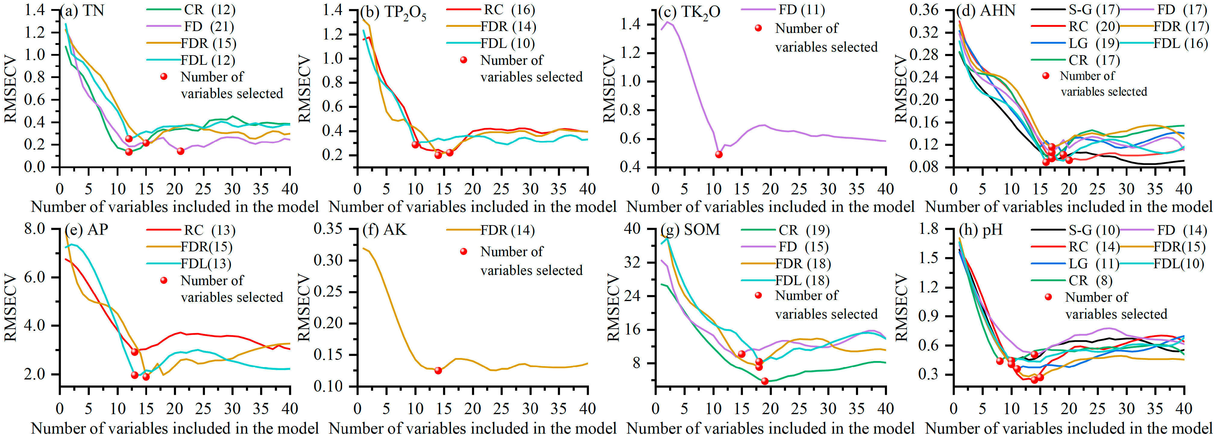
3.3. Feature Band Extraction

It can be seen from Section 3.2 that the enhancement of the correlation coefficients varies among different spectral transformation methods, and there is a negative enhancement. Therefore, combined with Table 1, the transformation methods with the maximum value of the absolute value of the correlation coefficient less than 0.6 were removed, and then the SPA was used to select the feature bands of the remaining spectra for modeling. The results of the SPA are shown in Figure 5 and Figure 6. Figure 5 shows the variation of the RMSECV with the increase in the number of variables during the screening of the feature bands, the number of variables finally selected, and the corresponding RMSECV. Figure 6 shows the location of the final screened feature bands. As seen from Figure 5, the RMSECV first decreased rapidly with the number of variables and then increased and stabilized during the SPA’s selection of the feature bands. The number of feature bands of the final different spectra ranged from 8 to 21, accounting for 1.14–3.0% of the full-band spectral data. From Figure 6 and Figure 4, it can be seen that the feature bands screened using the SPA are mainly concentrated in the region with high correlation, and the feature bands at this time have a good correlation with soil parameters and are suitable for subsequent modeling.

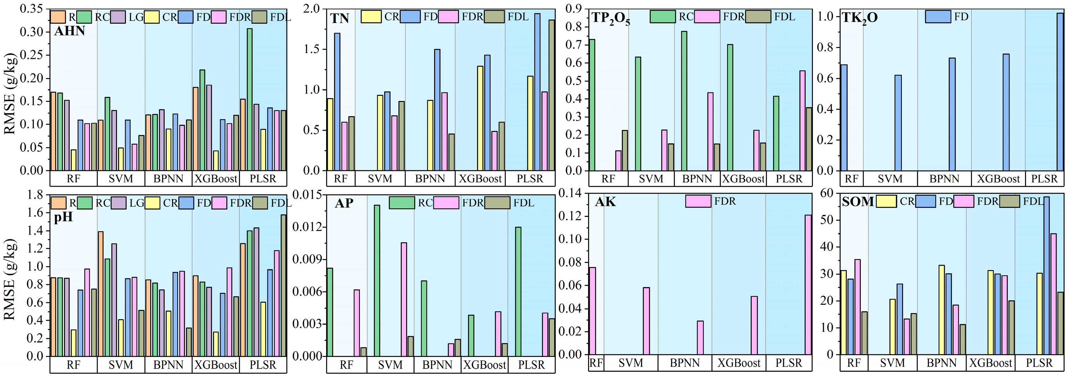
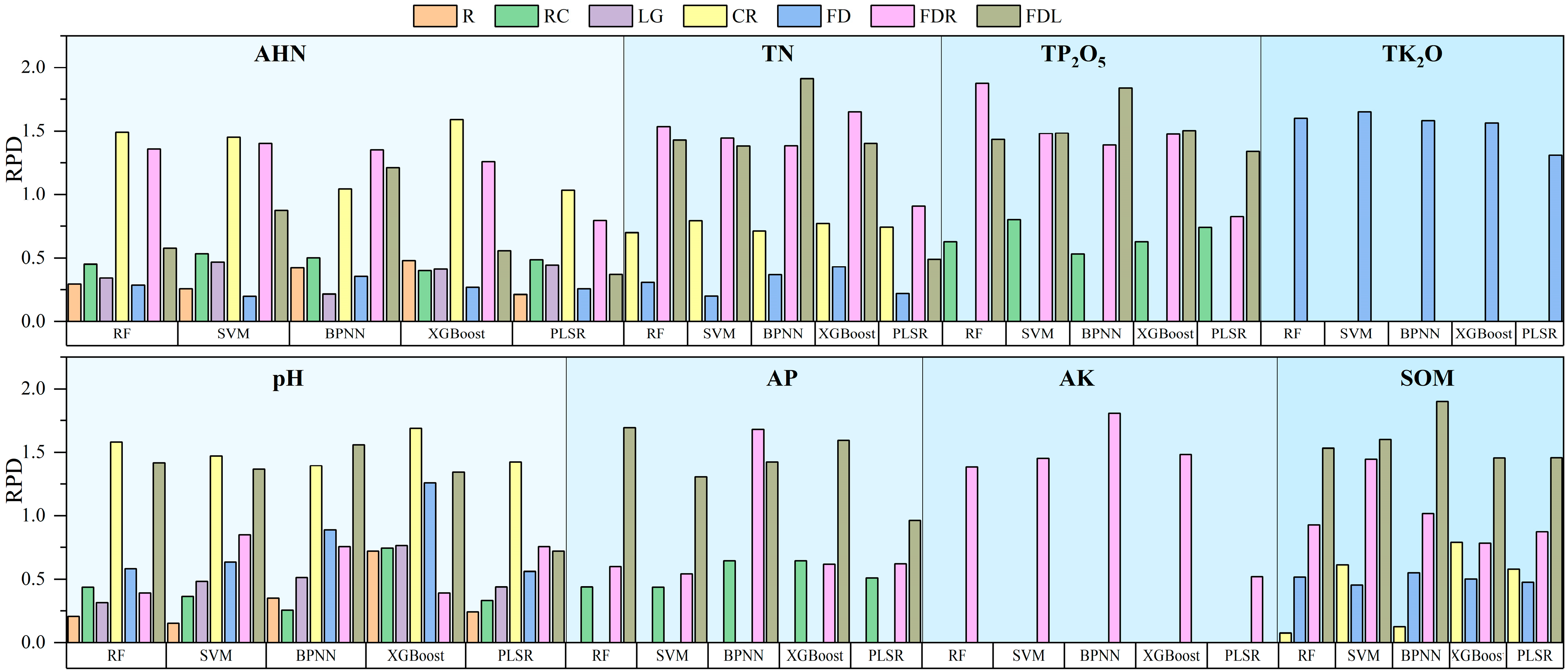
3.4. Model Performance Comparison

To enhance the model accuracy and compare the performance of the different models, this study used a random grid optimization search (5-fold cross-validation) to determine the optimal parameters within specified ranges for PLSR, RF, SVM, XGBoost, and BPNN. Subsequently, a total of 90 models were constructed using these optimal parameters. Detailed model hyperparameters are provided in the Supplementary Materials (Tables S1–S5). The evaluation of the model performance encompassed the calculation of R², RMSE, RPIQ, and RPD using 5-fold cross-validation on both the training and validation datasets. The results of the independent validation set are shown in Figure 7, Figure 8, Figure 9 and Figure 10.

As can be seen in Figure 7, Figure 8, Figure 9 and Figure 10, the PLSR model had the worst performance and could only achieve the prediction of SOM and pH (RPD and RPIQ > 1.4). Among the PLSR models predicting SOM and pH, the PLSR model built with SOM and FDL spectra had the highest accuracy (RPD = 1.458, RPIQ = 1.488), and the PLSR model built with pH and CR spectra had the best accuracy (RPD = 1.425, RPIQ = 1.570). The RF model can predict TN, AHN, SOM, pH, TP₂O₅, AP, and TK₂O. The SVM model has the ability to predict TN, AHN, SOM, pH, TP₂O₅, TK₂O, and AK. The XGBoost model can predict all parameters. Additionally, the BPNN model can predict TN, SOM, pH, TP₂O₅, AP, TK₂O, and AK (RPD > 1.4, RPIQ > 1.4). Among the soil TN prediction models, the order of the model accuracy is BPNN > XGBoost > RF > SVM, with the BPNN model utilizing the FDL transformation method. The validation set R² is 0.826, RMSE is 0.453 g/kg, RPD is 1.912, and RPIQ is 2.851. For AHN predictions, the order is XGBoost > RF > SVM > BPNN, with the XGBoost model utilizing the CR spectral transformation method. The validation set R² is 0.776, RMSE is 0.043 g/kg, RPD is 1.591, and RPIQ is 2.880, although BPNN is unable to predict AHN. In the case of SOM and AK prediction models, the model accuracy order is BPNN > SVM > RF > XGBoost and BPNN > XGBoost > SVM > RF, respectively, with validation RPD and RPIQ of 1.898, 3.085 and 1.806, 2.394, respectively. The RF model had the highest accuracy among all of the pH, AP, and TP₂O₅ prediction models, corresponding to RPDs of 1.58, 1.69, and 1.876 and RPIQs of 3.198, 3.011, and 2.776, respectively. In addition, SVM showed the best performance only in the prediction of TK₂O, and the worst was the BPNN model. Therefore, the above analysis reveals that in terms of the ability to predict the eight parameters, XGBoost can predict all of the parameters using soil spectra but only shows the best performance in the prediction of AHN. Therefore, XGBoost is the most universally applicable model. However, in terms of performance, RF had the highest accuracy in the prediction of three parameters—TP₂O₅, AP, and pH—and BPNN had the highest accuracy in the prediction of three parameters—TN, AK, and SOM—and they were the best models for these parameters. XGBoost and SVM performed best in predicting AHN and TK₂O, respectively. Finally, we statistically analyzed the prediction results of the best model for each parameter, which contains the maximum, minimum, mean, standard deviation, and coefficient of variation of the prediction set (Table S6). It also contains a boxplot of the prediction results (Figure S1). Therefore, when using soil spectral data to estimate soil parameters, the prediction performance of the same model for different parameters often has large differences, and it is necessary to choose the appropriate method according to the type of soil parameters [45].

Further analysis of the spectral transformation methods reveals that FDL and FDR transformations exhibited significant advantages over several other methods. These transformations improved the modeling and validation accuracy of the model effectively, while the FD and CR transformations also showed the potential to improve the model accuracy to some extent. However, the applicability of the different transformation methods varies because of the different soil parameters and models. For instance, while an RF model established using FDR spectral data can achieve TN prediction, the BPNN model cannot. As a result, the choice of spectral transformation methods needs to be tailored to different soil parameters and modeling approaches.

4. Discussion

Currently, despite some research progress in hyperspectral inversion of soil parameters in typical agricultural areas, forests, and industrial mining areas, there is a scarcity of studies on soil parameters in alpine meadows in ecologically fragile areas of the Qinghai–Tibet Plateau, and only a limited range of soil parameters have been involved [28,40,41,46,47,76,77,78]. The inversion models are mainly divided into linear and intelligent algorithm-based models, which apply to different regions. For example, Gao et al. [79] used MLSR, PLSR, and BPNN models to perform hyperspectral inversion of soil parameters in the Sanjiangyuan area in Qinghai province, China, but only a limited range of soil properties were involved (SOM and TN). Zhang et al. [80] studied the feasibility of Vis–NIR for predicting seven soil properties (SOM, TN, pH, CEC, clay, silt, and sand) with different variable screening methods. The results indicated that the model predicted these seven soil properties successfully, with SOM (R² = 0.81), TN (R² = 0.84), and pH (R² = 0.76) demonstrating the best prediction effect. The precision of SOM and pH is lower than our results (R² = 0.858, R² = 0.805) and the precision of TN is higher than ours (R² = 0.826). The results of Yang et al. [81], which are similar to those of Zhang et al.’s [80] studies conducted in small regions in other countries (e.g., the United States [82], Germany [25], and Thailand [83], have also found that the accuracy of SOM estimation is usually better than other parameters. In a large-scale survey (involving 23 EU member states) utilizing land use/land cover area frame survey (LUCAS) data, it was found that the pH estimation accuracy was generally higher than for organic carbon and cation exchange capacity [33]. In addition, studies on predictive models have found that more complex and intelligent algorithms have better results, e.g., utilizing deep learning algorithms is more effective than machine learning methods when there are sufficient samples [23,33,35,48,62]. On the other hand, deep learning algorithms often achieve the desired results without excessive data preprocessing steps.

SOM is the soil parameter with the highest prediction accuracy of Vis–NIR, and its overtones and combination bands in the Vis–NIR region are determined by the stretching and bending of N=H, C=H, and C=O groups [84]. Since TN is highly correlated with SOM and has a direct spectral response, it can be predicted by Vis–NIR. In addition, although AHN, TP₂O₅, and pH do not have apparent spectral response characteristics, they can still be predicted by Vis–NIR due to their correlation with SOM, TN, and some predictable properties, which is also confirmed in this study (Figure 7, Figure 8, Figure 9 and Figure 10). In addition, although the model can predict TK₂O, AP, and AK, the accuracy is poor. At the same time, the correct model and processing method need to be used, making prediction difficult. For the modeling methods, the overall ranking of model performance is as follows: RF > BPNN > SVM > PLSR, which is consistent with the findings of previous studies, but the order of XGBoost is usually not fixed [37,45,52,53]. The prediction of different soil parameters is different for different data preprocessing methods and modeling approaches. For example, the BPNN model constructed with FDL spectra predicts TN best, while the RF model constructed with FDR spectra predicts TP₂O₅ best. The difference between the same soil parameter and the different models built with the corresponding spectrum is usually not very large. For the same soil parameter, the difference in the prediction ability of different modeling methods may be due to the limitations of the model’s structure, parameter content, and data volume [23,81,85]. Further research and discussion are needed to understand the reasons for the difference in performance of different algorithms on the same soil parameter. This is also one of our future research goals.

The feature bands usually differ for different parameters, and different preprocessing methods and feature selection methods have different results. The results of the feature bands extracted in this study are shown in Figure 6. From the figure, we find that the different spectral transformation methods do not drastically change the feature bands of the soil parameters. Although the characteristic bands of the different transformed spectra corresponding to the same soil parameter vary, they tend to occur in similar ranges. This is because molecules and chemical bonds determine the spectral response to specific properties [36]. For soil TN, the characteristic bands screened were mainly focused on 450–850 nm, especially at around 550 nm, and 700–800 nm, similar to other studies’ findings. However, most of these studies used full-band spectra, and the final number of bands selected was higher [86,87,88]. In addition, for AP and AK, it was found that the featured bands of these parameters are mostly concentrated around 500 nm and 700–1000 nm, but there are some differences among different studies. For instance, Yu et al. [31] extracted the feature bands of AP and AK between 400–1100 nm using the SPA as 499, 516, 542, 745, and 770 nm and 556, 574, 595, 991, and 1013 nm, respectively, which are close to the findings of this study. Ren et al. [34] used the SPA to extract the bands of AP concentrated at 300–550 nm and AK near 250–600 nm, which was different from this and other studies. This may be due to the fact that their study was conducted on wetland soils, which are more different in nature from terrestrial soils. Studies using Vis–NIR to estimate SOM and pH found [30,81] that in the 400–1100 nm range, the characteristic bands of SOM were predominantly in the vicinity of 500–800 nm and 1000 nm, and pH in the vicinity of 700 nm and 1000 nm, which is also extremely close to the findings of the present study. However, there are few reports on selecting the feature bands of TP2O5 TK₂O, and AHN, which may be due to their similarities with TN, AK, and AP. Although they contain the same elements as TN, AK, and AP, they end up with differences in their characteristic bands due to the differences in some properties (e.g., content and chemical bonding).

The research area of this study was the alpine meadow in the source area of the Yellow River, but the area involved was mainly six sample plots in this area, and the scope of the study was limited. Therefore, because of constraints such as the limited number of samples used in the present work and challenges like large-scale monitoring and high altitude, the model’s applicability to other unsampled areas in the Yellow River source area still need to be verified. The spectral preprocessing methods we used were mostly simple mathematical transformations, which could not dig deeper into the deep information, as well as remove the influence of the background in the spectra, and the performance improvement of the model was limited. For the feature selection algorithm, we only used SPA without further comparative analysis of other methods, such as optimization algorithms, dimensionality reduction algorithms, and other screening algorithms. In future works, more advanced and sophisticated methods can be employed and compared, such as the standard normal transform, multivariate scattering correction, wavelet transform, and detrending, as well as their combined usage. An increased number of soil samples can be collected from a wider area to enhance the model’s applicability, and the optimization of feature band extraction and modeling methods can be pursued to heighten the model accuracy. Meanwhile, more complex and multivariate models should be selected, for example, one-dimensional convolutional neural networks, deep neural networks, and recurrent neural networks in deep learning models [35,48,49,62]; extreme learning machine, Gaussian process regression, etc., in machine learning. The parameters and structure of these models can also be optimized for better results. Additionally, the inversion of multiple parameters of alpine meadow soils can be investigated by combining hyperspectral imaging and unmanned aerial vehicles (UAVs) to obtain the spatial distribution of soil nutrients on a large scale. This approach can offer technical and data support for the monitoring and restoration of degradation, as well as for agricultural and livestock production, within alpine meadows in the Yellow River source area.

5. Conclusions

This study investigated the predictability and accuracy of Vis–NIR in predicting AHN, AK, AP, SOM, TN, TK₂O, TP₂O₅, and pH contents in alpine meadow soils. We improved the correlation between the spectrum and different parameters by applying the mathematical transformation to the spectrum and eliminating the transformation methods whose correlation was lower than the threshold. Then, the SPA was employed to screen the characteristic bands of the remaining spectra, and the PLSR, RF, SVM, XGBoost, and BPNN algorithms were utilized to model. The results revealed that mathematical transformation can enhance spectral characteristics and improve the correlation between spectral data and soil parameters. However, the effect on different parameters varies. The effect of the CR, DF, FDR, and FDL transforms is superior to that of other transformation methods. The PLSR, RF, SVM, XGBoost, and BPNN methods were used to construct the prediction model and optimize its hyperparameters. Finally, the model’s accuracy was evaluated using 5-fold cross-validation. It was observed that the PLSR model only enables the prediction of SOM and pH with lower accuracy than the remaining four models. XGBoost has the ability to predict all parameters. The RF model could predict seven out of eight parameters, excluding AK. The SVM model could predict parameters, excluding AP, and the BPNN model could predict parameters, excluding AHN. However, the RF model demonstrated a higher accuracy in predicting TP₂O₅, AP, and pH compared with the other four methods. The BPNN model showed the highest accuracy in predicting TN, AK, and SOM. SVM exhibited higher accuracy only in predicting TK₂O and XGBoost in AHN. Using the correlation coefficient threshold method to remove transformation modes with low correlation is beneficial for efficient modeling. Additionally, the feature selection algorithm can effectively select the information-rich spectral bands, diminish the spectral data dimension, and establish a more comprehensive model.

In summary, this study showcased the feasibility and accuracy of employing Vis–NIR to predict the contents of AHN, AK, AP, SOM, TN, TK₂O, TP₂O₅, and pH within alpine meadow soil. This outcome lays a foundation for the monitoring and management of alpine meadow soil status.

References

1. Adhikari, K.; Hartemink, A.E. Linking soils to ecosystem services—A global review. Geoderma 2016, 262, 101–111. [Google Scholar] [CrossRef]
2. Yang, Z.J.; Chen, X.M.; Jing, F.; Guo, B.L.; Lin, G.Z. Spatial variability of nutrients and heavy metals in paddy field soils based on GIS and Geostatistics. Ying Yong Sheng Tai Xue Bao J. Appl. Ecol. 2018, 29, 1893–1901. [Google Scholar]
3. Man, Z.H. Monitoring Study on Alpine Meadow Response to Freezing-Thawing Events in the Nagqu River Basin. Master’s Thesis, Hebei University of Engineering, Handan, China, 2020. [Google Scholar]
4. Qiu, J. China: The third pole. Nature 2008, 454, 393–396. [Google Scholar] [CrossRef] [PubMed]
5. Qin, Q.T.; Chen, J.J.; Yang, Y.P.; Zhao, X.Y.; Zhou, G.Q.; You, H.T.; Han, X.W. Spatiotemporal variations of vegetation and its response to topography and climate in the source region of the Yellow River. China Environ. Sci. 2021, 41, 3832–3841. [Google Scholar]
6. Li, C.Y.; Zhang, W.J.; Lai, Z.M.; Peng, F.; Chen, X.J.; Xue, X.; Wang, T.; You, Q.G.; Du, H.Q. Plant productivity, species diversity, soil properties, and their relationships in an alpine steppe under different degradation degress at the source of the Yellow River. Acta Evologica Sin. 2021, 41, 4541–4551. [Google Scholar]
7. Zhao, J.; Jiang, C.; Ding, Y.; Peng, J. Alpine vegetation coverage mutation and its attribution analysis based on AVHRR NDVI data. In Proceedings of the Fourth International Conference on Geoscience and Remote Sensing Mapping (GRSM 2022), Changchun, China, 21–23 October 2022; p. 125512X. [Google Scholar]
8. Chen, H.; Ju, P.; Zhu, Q.; Xu, X.; Wu, N.; Gao, Y.; Feng, X.; Tian, J.; Niu, S.; Zhang, Y.; et al. Carbon and nitrogen cycling on the Qinghai–Tibetan Plateau. Nat. Rev. Earth Environ. 2022, 3, 701–716. [Google Scholar] [CrossRef]
9. Xu, Y.-d.; Dong, S.-k.; Shen, H.; Xiao, J.-n.; Li, S.; Gao, X.-x.; Wu, S.-n. Degradation significantly decreased the ecosystem multifunctionality of three alpine grasslands: Evidences from a large-scale survey on the Qinghai-Tibetan Plateau. J. Mt. Sci. 2021, 18, 357–366. [Google Scholar] [CrossRef]
10. Li, H.; Qiu, Y.; Yao, T.; Han, D.; Gao, Y.; Zhang, J.; Ma, Y.; Zhang, H.; Yang, X. Nutrients available in the soil regulate the changes of soil microbial community alongside degradation of alpine meadows in the northeast of the Qinghai-Tibet Plateau. Sci. Total Environ. 2021, 792, 148363. [Google Scholar] [CrossRef] [PubMed]
11. Wu, J.; Wang, H.; Li, G.; Ma, W.; Wu, J.; Gong, Y.; Xu, G. Vegetation degradation impacts soil nutrients and enzyme activities in wet meadow on the Qinghai-Tibet Plateau. Sci. Rep. 2020, 10, 21271. [Google Scholar] [CrossRef] [PubMed]
12. Zhang, W.; Xue, X.; Peng, F.; You, Q.; Hao, A. Meta-analysis of the effects of grassland degradation on plant and soil properties in the alpine meadows of the Qinghai-Tibetan Plateau. Glob. Ecol. Conserv. 2019, 20, e00774. [Google Scholar] [CrossRef]
13. Jianyun, Z.; Chuanli, J.; Wenhui, L.; Yuanyuan, D.; Guorong, L. Pika disturbance intensity observation system via multidimensional stereoscopic surveying for monitoring alpine meadow. J. Appl. Remote Sens. 2022, 16, 044524. [Google Scholar]
14. Xie, S.; Ding, F.; Chen, S.; Wang, X.; Li, Y.; Ma, K. Prediction of soil organic matter content based on characteristic band selection method. Spectrochim. Acta Part A Mol. Biomol. Spectrosc. 2022, 273, 120949. [Google Scholar] [CrossRef] [PubMed]
15. Hayashi, K. Nitrogen cycling and management focusing on the central role of soils: A review. Soil Sci. Plant Nutr. 2022, 68, 514–525. [Google Scholar] [CrossRef]
16. Devianti; Sufardi; Bulan, R.; Sitorus, A. Vis-NIR spectra combined with machine learning for predicting soil nutrients in cropland from Aceh Province, Indonesia. Case Stud. Chem. Environ. Eng. 2022, 6, 100268. [Google Scholar] [CrossRef]
17. Sardans, J.; Bartrons, M.; Margalef, O.; Gargallo-Garriga, A.; Janssens, I.A.; Ciais, P.; Obersteiner, M.; Sigurdsson, B.D.; Chen, H.Y.H.; Peñuelas, J. Plant invasion is associated with higher plant–soil nutrient concentrations in nutrient-poor environments. Glob. Chang. Biol. 2017, 23, 1282–1291. [Google Scholar] [CrossRef]
18. Wang, Y.C.; Yang, X.F.; Zhao, Q.C.; Gu, X.H.; Guo, C.; Liu, Y.P. Quantitative inversion of soil organic matter content in northern alluvial soil based on binary wavelet transform. Spectrosc. Spectr. Anal. 2019, 39, 2855–2861. [Google Scholar]
19. Zhong, H.; Li, X.C.; Zhai, H.R.; Zhou, Y. Hyperspectral indirect estimation model of soil organic matter content in plough layer. J. Geomat. Sci. Technol. 2019, 36, 74–78+85. [Google Scholar]
20. Zhang, C.; Xie, Z. Object-based vegetation mapping in the Kissimmee River watershed using HyMap data and machine learning techniques. Wetlands 2013, 33, 233–244. [Google Scholar] [CrossRef]
21. Selige, T.; Böhner, J.; Schmidhalter, U. High resolution topsoil mapping using hyperspectral image and field data in multivariate regression modeling procedures. Geoderma 2006, 136, 235–244. [Google Scholar] [CrossRef]
22. Jiang, Y.L.; Wang, R.H.; Li, Y.; Li, C.; Peng, Q.; Wu, X.Q. Hypersperctral retrieval of soil nutrient content of various land-cover types in Ebinur Lake Basin. Chin. J. Eco-Agric. 2016, 24, 1555–1564. [Google Scholar]
23. Wang, Y.; Li, M.; Ji, R.; Wang, M.; Zheng, L. Comparison of Soil Total Nitrogen Content Prediction Models Based on Vis-NIR Spectroscopy. Sensors 2020, 20, 7078. [Google Scholar] [CrossRef]
24. Zhou, P.; Zhang, Y.; Yang, W.; Li, M.; Liu, Z.; Liu, X. Development and performance test of an in-situ soil total nitrogen-soil moisture detector based on near-infrared spectroscopy. Comput. Electron. Agric. 2019, 160, 51–58. [Google Scholar] [CrossRef]
25. Morellos, A.; Pantazi, X.-E.; Moshou, D.; Alexandridis, T.; Whetton, R.; Tziotzios, G.; Wiebensohn, J.; Bill, R.; Mouazen, A.M. Machine learning based prediction of soil total nitrogen, organic carbon and moisture content by using VIS-NIR spectroscopy. Biosyst. Eng. 2016, 152, 104–116. [Google Scholar] [CrossRef]
26. Peng, Y.; Wang, T.; Xie, S.; Liu, Z.; Lin, C.; Hu, Y.; Wang, J.; Mao, X. Estimation of Soil Cations Based on Visible and Near-Infrared Spectroscopy and Machine Learning. Agriculture 2023, 13, 1237. [Google Scholar] [CrossRef]
27. Akter, S.; de Jonge, L.W.; Møldrup, P.; Greve, M.H.; Nørgaard, T.; Weber, P.L.; Hermansen, C.; Mouazen, A.M.; Knadel, M. Visible Near-Infrared Spectroscopy and Pedotransfer Function Well Predict Soil Sorption Coefficient of Glyphosate. Remote Sens. 2023, 15, 1712. [Google Scholar] [CrossRef]
28. Juanjuan, Z.; Qinqin, W.; Shuping, X.; Lei, S.; Xinming, M.; Pan, D.; Jianbiao, G. A spectral parameter for the estimation of soil total nitrogen and nitrate nitrogen of winter wheat growth period. Soil Use Manag. 2020, 37, 698–711. [Google Scholar]
29. El-Sayed, M.A.; Abd-Elazem, A.H.; Moursy, A.R.A.; Mohamed, E.S.; Kucher, D.E.; Fadl, M.E. Integration Vis-NIR Spectroscopy and Artificial Intelligence to Predict Some Soil Parameters in Arid Region: A Case Study of Wadi Elkobaneyya, South Egypt. Agronomy 2023, 13, 935. [Google Scholar] [CrossRef]
30. Wang, L.; Wang, R. Determination of soil pH from Vis-NIR spectroscopy by extreme learning machine and variable selection: A case study in lime concretion black soil. Spectrochim. Acta Part A Mol. Biomol. Spectrosc. 2022, 283, 121707. [Google Scholar] [CrossRef]
31. Yu, B.; Yan, C.; Yuan, J.; Ding, N.; Chen, Z. Prediction of soil properties based on characteristic wavelengths with optimal spectral resolution by using Vis-NIR spectroscopy. Spectrochim. Acta Part A Mol. Biomol. Spectrosc. 2023, 293, 122452. [Google Scholar] [CrossRef]
32. Zhou, P.; Sudduth, K.A.; Veum, K.S.; Li, M. Extraction of reflectance spectra features for estimation of surface, subsurface, and profile soil properties. Comput. Electron. Agric. 2022, 196, 106845. [Google Scholar] [CrossRef]
33. Yang, J.; Wang, X.; Wang, R.; Wang, H. Combination of Convolutional Neural Networks and Recurrent Neural Networks for predicting soil properties using Vis–NIR spectroscopy. Geoderma 2020, 380, 114616. [Google Scholar] [CrossRef]
34. Ren, G.X.; Wei, Z.Q.; Fan, P.P.; Wang, X.Y. Visible/near infrared spectroscopy method applied research in wetland soil nutrients rapid test. IOP Conf. Ser. Earth Environ. Sci. 2019, 344, 012123. [Google Scholar] [CrossRef]
35. Kawamura, K.; Nishigaki, T.; Andriamananjara, A.; Rakotonindrina, H.; Tsujimoto, Y.; Moritsuka, N.; Rabenarivo, M.; Razafimbelo, T. Using a One-Dimensional Convolutional Neural Network on Visible and Near-Infrared Spectroscopy to Improve Soil Phosphorus Prediction in Madagascar. Remote Sens. 2021, 13, 1519. [Google Scholar] [CrossRef]
36. Xiaobo, Z.; Jiewen, Z.; Povey, M.J.W.; Holmes, M.; Hanpin, M. Variables selection methods in near-infrared spectroscopy. Anal. Chim. Acta 2010, 667, 14–32. [Google Scholar] [CrossRef]
37. Liu, L.; Ji, M.; Dong, Y.; Zhang, R.; Buchroithner, M. Quantitative Retrieval of Organic Soil Properties from Visible Near-Infrared Shortwave Infrared (Vis-NIR-SWIR) Spectroscopy Using Fractal-Based Feature Extraction. Remote Sens. 2016, 8, 1035. [Google Scholar] [CrossRef]
38. Li, J.; Zhang, H.; Zhan, B.; Zhang, Y.; Li, R.; Li, J. Nondestructive firmness measurement of the multiple cultivars of pears by Vis-NIR spectroscopy coupled with multivariate calibration analysis and MC-UVE-SPA method. Infrared Phys. Technol. 2020, 104, 103154. [Google Scholar]
39. Jiang, C.L.; Zhao, J.Y.; Ding, Y.Y.; Zhao, Q.H.; Ma, H.Y. Study on Soil Water Retrieval Technology of Yellow River Source Based on SPA Algorithm and Machine Learning. Spectrosc. Spectr. Anal. 2023, 43, 1961–1967. [Google Scholar]
40. Zhang, C.; Liu, Y.M.; Sun, Y.N.; Wang, L.; Liu, J.H. Hyperspectral prediction model of soil nutrient content in the loess hilly-gully region, China. Chin. J. Appl. Ecol. 2018, 29, 2835–2842. [Google Scholar]
41. Lin, N.; Liu, H.Q.; Yang, J.J.; Wu, M.H.; Liu, H.L. Hyperspectral estimation of soil nutrient content in the black soil region based on BA-Adaboost. Spectrosc. Spectr. Anal. 2020, 40, 3825–3831. [Google Scholar]
42. Pudełko, A.; Chodak, M.; Roemer, J.; Uhl, T. Application of FT-NIR spectroscopy and NIR hyperspectral imaging to predict nitrogen and organic carbon contents in mine soils. Measurement 2020, 164, 108117. [Google Scholar] [CrossRef]
43. Yang, R.-M. Characterization of the salt marsh soils and visible-near-infrared spectroscopy along a chronosequence of Spartina alterniflora invasion in a coastal wetland of eastern China. Geoderma 2020, 362, 114138. [Google Scholar] [CrossRef]
44. Kawamura, K.; Nishigaki, T.; Tsujimoto, Y.; Andriamananjara, A.; Rabenaribo, M.; Asai, H.; Rakotoson, T.; Razafimbelo, T. Exploring relevant wavelength regions for estimating soil total carbon contents of rice fields in Madagascar from Vis-NIR spectra with sequential application of backward interval PLS. Plant Prod. Sci. 2021, 24, 1–14. [Google Scholar] [CrossRef]
45. Peng, Y.; Zhao, L.; Hu, Y.; Wang, G.; Wang, L.; Liu, Z. Prediction of Soil Nutrient Contents Using Visible and Near-Infrared Reflectance Spectroscopy. ISPRS Int. J. Geo-Inf. 2019, 8, 437. [Google Scholar] [CrossRef]
46. Xie, W. Study on Spectral Characteristics and Estimation Models of Different Nutrient Contents in Forest Soils Based on Hyperspectral Techonlogy. Ph.D. Thesis, Jiangxi Agricultural University, Nanchang, China, 2017. [Google Scholar]
47. Yang, Y.C.; Zhao, Y.J.; Qin, K.; Zhao, N.B.; Yang, C.; Zhang, D.H.; Cui, X. Prediction of black soil nutrient content based on airborne hyperspectral remote sensing. Trans. Chin. Soc. Agric. Eng. 2019, 35, 94–101. [Google Scholar]
48. Blazhko, U.; Shapaval, V.; Kovalev, V.; Kohler, A. Comparison of augmentation and pre-processing for deep learning and chemometric classification of infrared spectra. Chemom. Intell. Lab. Syst. 2021, 215, 104367. [Google Scholar] [CrossRef]
49. Sun, J.; Wang, G.; Zhang, H.; Xia, L.; Zhao, W.; Guo, Y.; Sun, X. Detection of fat content in peanut kernels based on chemometrics and hyperspectral imaging technology. Infrared Phys. Technol. 2020, 105, 103226. [Google Scholar] [CrossRef]
50. Alkesaiberi, A.; Harrou, F.; Sun, Y. Efficient Wind Power Prediction Using Machine Learning Methods: A Comparative Study. Energies 2022, 15, 2327. [Google Scholar] [CrossRef]
51. Pan, Q.; Harrou, F.; Sun, Y. A comparison of machine learning methods for ozone pollution prediction. J. Big Data 2023, 10, 63. [Google Scholar] [CrossRef]
52. Chen, S.; Lou, F.; Tuo, Y.; Tan, S.; Peng, K.; Zhang, S.; Wang, Q. Prediction of Soil Water Content Based on Hyperspectral Reflectance Combined with Competitive Adaptive Reweighted Sampling and Random Frog Feature Extraction and the Back-Propagation Artificial Neural Network Method. Water 2023, 15, 935. [Google Scholar] [CrossRef]
53. Tan, B.; You, W.; Tian, S.; Xiao, T.; Wang, M.; Zheng, B.; Luo, L. Soil Nitrogen Content Detection Based on Near-Infrared Spectroscopy. Sensors 2022, 22, 8013. [Google Scholar] [CrossRef]
54. Zhao, J.Y.; Ding, Y.Y.; Du, M.; Liu, W.H.; Zhu, H.L.; Li, G.R.; Yang, J. Vegetation coverage inversion of alpine grassland in the source of the Yellow River based on unmanned aerial vehicle and machine learning. Sci. Technol. Eng. 2021, 21, 10209–10214. [Google Scholar]
55. Zhen, Z.Y.; Lv, M.X.; Ma, Z.G. Climate, hydrology, and vegetation coverage changes in source region of Yellow River and countermeasures for challenges. Bull. Chin. Acad. Sci. 2020, 35, 61–72. [Google Scholar]
56. Wu, X.F.; Li, G.X.; Pan, X.P.; Wang, Y.F.; Zhang, S.; Liu, F.G.; Shen, Y.J. Response of vegetation cover to temperature and precipitation in the source region of the Yellow River. Resour. Sci. 2015, 37, 512–521. [Google Scholar]
57. Yang, R.R. Spatio-Temporal Variation of Vegetation Coverage and Its Response to Climate Change in the Source Region of the Yellow River from 2000 to 2017. Master’s Thesis, Chengdu University of Technology, Chengdu, China, 2019. [Google Scholar]
58. Shi, D.D.; Yand, T.; Hu, J.M.; Gu, Z.J.; Jia, H.F. Spatio-temporal variation of NDVI-based wegetation during the growing-season and its relation with climatic factiors in the Yellow River Source Region. Mt. Res. 2018, 36, 184–193. [Google Scholar]
59. Wan, B.; Mei, X.; Hu, Z.; Guo, H.; Chen, X.; Griffiths, B.S.; Liu, M. Moderate grazing increases the structural complexity of soil micro-food webs by promoting root quantity and quality in a Tibetan alpine meadow. Appl. Soil Ecol. 2021, 168, 104161. [Google Scholar] [CrossRef]
60. Li, X.; Zhang, X.; Wu, J.; Shen, Z.; Zhang, Y.; Xu, X.; Fan, Y.; Zhao, Y.; Yan, W. Root biomass distribution in alpine ecosystems of the northern Tibetan Plateau. Environ. Earth Sci. 2011, 64, 1911–1919. [Google Scholar] [CrossRef]
61. Su, P.; Zhou, Z.; Shi, R.; Xie, T. Variation in basic properties and carbon sequestration capacity of an alpine sod layer along moisture and elevation gradients. Acta Ecol. Sin. 2018, 38, 1040–1052. [Google Scholar]
62. Jiang, C.; Zhao, J.; Ding, Y.; Li, G. Vis-NIR Spectroscopy Combined with GAN Data Augmentation for Predicting Soil Nutrients in Degraded Alpine Meadows on the Qinghai-Tibet Plateau. Sensors 2023, 23, 3686. [Google Scholar] [CrossRef]
63. Zhu, H.; Chu, B.; Zhang, C.; Liu, F.; Jiang, L.; He, Y. Hyperspectral Imaging for Presymptomatic Detection of Tobacco Disease with Successive Projections Algorithm and Machine-learning Classifiers. Sci. Rep. 2017, 7, 4125. [Google Scholar] [CrossRef]
64. Kamruzzaman, M.; Kalita, D.; Ahmed, M.T.; ElMasry, G.; Makino, Y. Effect of variable selection algorithms on model performance for predicting moisture content in biological materials using spectral data. Anal. Chim. Acta 2022, 1202, 339390. [Google Scholar] [CrossRef] [PubMed]
65. Soares, S.F.C.; Gomes, A.A.; Araujo, M.C.U.; Filho, A.R.G.; Galvão, R.K.H. The successive projections algorithm. TrAC Trends Anal. Chem. 2013, 42, 84–98. [Google Scholar] [CrossRef]
66. Breiman, L. Random Forests. Mach. Learn. 2001, 45, 5–32. [Google Scholar] [CrossRef]
67. Dai, L.; Ge, J.; Wang, L.; Zhang, Q.; Liang, T.; Bolan, N.; Lischeid, G.; Rinklebe, J. Influence of soil properties, topography, and land cover on soil organic carbon and total nitrogen concentration: A case study in Qinghai-Tibet plateau based on random forest regression and structural equation modeling. Sci. Total Environ. 2022, 821, 153440. [Google Scholar] [CrossRef] [PubMed]
68. Xiao, T.; Segoni, S.; Liang, X.; Yin, K.; Casagli, N. Generating soil thickness maps by means of geomorphological-empirical approach and random forest algorithm in Wanzhou County, Three Gorges Reservoir. Geosci. Front. 2023, 14, 101514. [Google Scholar] [CrossRef]
69. Bansal, M.; Goyal, A.; Choudhary, A. A comparative analysis of K-Nearest Neighbor, Genetic, Support Vector Machine, Decision Tree, and Long Short Term Memory algorithms in machine learning. Decis. Anal. J. 2022, 3, 100071. [Google Scholar] [CrossRef]
70. He, B.; Jia, B.; Zhao, Y.; Wang, X.; Wei, M.; Dietzel, R. Estimate soil moisture of maize by combining support vector machine and chaotic whale optimization algorithm. Agric. Water Manag. 2022, 267, 107618. [Google Scholar] [CrossRef]
71. Zhu, Q.; Wang, Y.; Luo, Y. Improvement of multi-layer soil moisture prediction using support vector machines and ensemble Kalman filter coupled with remote sensing soil moisture datasets over an agriculture dominant basin in China. Hydrol. Process. 2021, 35, e14154. [Google Scholar] [CrossRef]
72. Friedman, J.H. Greedy Function Approximation: A Gradient Boosting Machine. Ann. Stat. 2001, 29, 1189–1232. [Google Scholar] [CrossRef]
73. Chollet, F. Keras. 2015. Available online: https://github.com/keras-team/keras (accessed on 15 August 2023).
74. Pedregosa, F.; Varoquaux, G.; Gramfort, A.; Michel, V.; Thirion, B.; Grisel, O. Scikit-Learn: Machine Learning in Python. Available online: https://github.com/scikit-learn/scikit-learn (accessed on 15 August 2023).
75. Liu, J.; Han, J.; Xie, J.; Wang, H.; Tong, W.; Ba, Y. Assessing heavy metal concentrations in earth-cumulic-orthic-anthrosols soils using Vis-NIR spectroscopy transform coupled with chemometrics. Spectrochim. Acta Part A Mol. Biomol. Spectrosc. 2020, 226, 117639. [Google Scholar] [CrossRef]
76. Zhang, D.H.; Zhao, Y.J.; Qin, K. A new model for predicting black soil nutrient content by spectral parameters. Spectrosc. Spectr. Anal. 2018, 38, 2932–2936. [Google Scholar]
77. Zhang, D.H.; Qin, K.; Zhao, Y.J.; Zhao, N.B.; Yang, Y.C. Influence of spectral transformation methods on nutrient content inversion accuracy by hyperspectral remote sensing in black soil. Trans. Chin. Soc. Agric. Eng. 2018, 34, 141–147. [Google Scholar]
78. Cheng, X.F.; Song, T.T.; Chen, Y.; Wei, Y.M.; Shen, J.X.; Qi, W.F. Retrieval and analysis of heavy metal content in soil based on measured spectrain the Lanping Zn-Pb mining area, western Yunnan Province. Acta Petrol. Et Mineral. 2017, 36, 60–69. [Google Scholar]
79. Gao, X.; Yang, Y.; Zhang, W.; Jia, W.; Li, J.; Tian, C.; Zhang, Y.; He, L. Visible-near infrared reflectance spectroscopy for estimating soil total nitrogen contents in the Sanjiang Yuan Regions, China: A case study of Yushu County and Maduo County, Qinghai province. In Proceedings of the SPIE Asia-Pacific Remote Sensing, Beijing, China, 13–16 October 2014; p. 92631O. [Google Scholar]
80. Zhang, X.; Xue, J.; Xiao, Y.; Shi, Z.; Chen, S. Towards Optimal Variable Selection Methods for Soil Property Prediction Using a Regional Soil Vis-NIR Spectral Library. Remote Sens. 2023, 15, 465. [Google Scholar] [CrossRef]
81. Yang, M.; Xu, D.; Chen, S.; Li, H.; Shi, Z. Evaluation of Machine Learning Approaches to Predict Soil Organic Matter and pH Using vis-NIR Spectra. Sensors 2019, 19, 263. [Google Scholar] [CrossRef] [PubMed]
82. Dhawale, N.M.; Adamchuk, V.I.; Prasher, S.O.; Viscarra Rossel, R.A. Evaluating the Precision and Accuracy of Proximal Soil vis–NIR Sensors for Estimating Soil Organic Matter and Texture. Soil Syst. 2021, 5, 48. [Google Scholar] [CrossRef]
83. Nawar, S.; Buddenbaum, H.; Hill, J.; Kozak, J.; Mouazen, A.M. Estimating the soil clay content and organic matter by means of different calibration methods of vis-NIR diffuse reflectance spectroscopy. Soil Tillage Res. 2016, 155, 510–522. [Google Scholar] [CrossRef]
84. Stenberg, B.; Viscarra Rossel, R.A.; Mouazen, A.M.; Wetterlind, J. Chapter Five—Visible and Near Infrared Spectroscopy in Soil Science. Adv. Agron. 2010, 107, 163–215. [Google Scholar]
85. Zhao, D.; Arshad, M.; Wang, J.; Triantafilis, J. Soil exchangeable cations estimation using Vis-NIR spectroscopy in different depths: Effects of multiple calibration models and spiking. Comput. Electron. Agric. 2021, 182, 105990. [Google Scholar] [CrossRef]
86. Cheng, H.; Wang, J.; Du, Y. Combining multivariate method and spectral variable selection for soil total nitrogen estimation by Vis–NIR spectroscopy. Arch. Agron. Soil Sci. 2021, 67, 1665–1678. [Google Scholar] [CrossRef]
87. Chen, Z.; Ren, S.; Qin, R.; Nie, P. Rapid Detection of Different Types of Soil Nitrogen Using Near-Infrared Hyperspectral Imaging. Molecules 2022, 27, 2017. [Google Scholar] [CrossRef]
88. Kawamura, K.; Tsujimoto, Y.; Rabenarivo, M.; Asai, H.; Andriamananjara, A.; Rakotoson, T. Vis-NIR Spectroscopy and PLS Regression with Waveband Selection for Estimating the Total C and N of Paddy Soils in Madagascar. Remote Sens. 2017, 9, 1081. [Google Scholar] [CrossRef]
Figure 1. Geographical location, elevation, and sampling area distribution of the study area.
Agronomy 13 02816 g001
Figure 2. Technical roadmap of the research.
Agronomy 13 02816 g002
Figure 3. Soil Vis–NIR spectrum and its transformation.
Agronomy 13 02816 g003
Figure 4. Heat map of the correlation coefficients between the soil parameters and spectra of different transformation forms. The correlation coefficients of soil TN, TP2O5, TK2O, AHN, AP, AK, SOM, and pH with the corresponding spectra (from left to right, S–G, LG, RC, FD, CR, FDR, FDL) are shown from top to bottom.
Agronomy 13 02816 g004
Figure 5. Variation of the RMSECV with the number of variables in the SPA band selection process.
Agronomy 13 02816 g005
Figure 6. SPA results of selected feature band.
Agronomy 13 02816 g006
Figure 7. R2 on independent validation sets for all models.
Agronomy 13 02816 g007
Figure 8. RMSE on independent validation sets for all models. Note that pH has no units.
Agronomy 13 02816 g008
Figure 9. RPD on independent validation sets for all models.
Agronomy 13 02816 g009
Figure 10. RPIQ on independent validation sets for all models.
Agronomy 13 02816 g010