Abstract
Due to the heavy computation load of closed-loop simulations, optimal control of greenhouse climate is usually simulated in an open-loop form to produce control strategies and profit indicators. Open-loop simulations assume the model, measurements, and predictions to be perfect, resulting in too-idealistic indicators. The method of two-time-scale decomposition reduces the computation load, thus facilitating the online implementation of optimal control algorithms. However, the computation time of nonlinear dynamic programming is seldom considered in closed-loop simulations. This paper develops a two-time-scale decomposed closed-loop optimal control algorithm that involves the computation time. The obtained simulation results are closer to reality since it considers the time delay in the implementation. With this algorithm, optimal control of Venlo greenhouse lettuce cultivation is investigated in Lhasa. Results show that compared with open-loop simulations, the corrections in yield and profit indicators can be up to 2.38 kg m−2 and 11.01 CNY m−2, respectively, through closed-loop simulations without considering the computation time. When involving the time delay caused by the computation time, further corrections in yield and profit indicators can be up to 0.1 kg m−2 and 0.87 CNY m−2, respectively. These conservative indicators help investors make wiser decisions before cultivation. Moreover, control inputs and greenhouse climate states are within their bounds most of the time during closed-loop simulations. This verifies that the developed algorithm can be implemented in real time.
1. Introduction
The greenhouse system involves the interaction between climate and crop [1]. Thus, climate control is the fundamental way to guarantee crop yield and quality. The usual method of climate control is to determine the climate setpoints based on growers’ experience, and then track the setpoints through feedback control [2]. However, manual settings cannot ensure meeting the requirements of crop growth and energy reduction. Optimal control realizes the maximization or minimization of the control objective based on the system dynamic model. However, there are two time-scales in the greenhouse system. Crop growth operates at the “day” level, while greenhouse climate operates at the “minute” level [3]. Thus, optimal control of greenhouse climate usually employs the strategy of hierarchical control, dividing the control system into “optimal-level” and “control-level”. Setpoint trajectories are optimized at the “optimal-level”, while setpoint trajectories are tracked at the “control-level” [4]. However, setpoint trajectories are determined by the long-term weather predictions, which are different from the real weather data in the implementation [5]. Thus, tracking setpoint trajectories optimized with the long-term weather predictions leads to high energy costs. To handle this problem, Van Henten and Bontsema [3] introduced the method of two-time-scale decomposition, which uses the crop state trajectory and costate trajectory optimized at the “optimal-level” as parts of the control objective at the “control-level”. In this way, the control performance loss caused by long-term weather prediction errors is reduced through more accurate short-term weather predictions at the “control-level”. This realizes the decomposition of “optimal-level” and “control-level”.
Open-loop simulations at the “optimal-level” compute only once, costing a relatively short computation time. Thus, current research on optimal control of greenhouse climate usually produces control strategies through open-loop simulations to guide cultivation. Due to the problem of two time-scales, most research minimized the energy cost based on the greenhouse climate deterministic model [6]. Van Beveren et al. [7] produced the open-loop optimal control strategies of the combined heat and power device based on the greenhouse heating and cooling requirements, resulting in a reduction of 29% in energy costs. Lin et al. [8] produced open-loop optimal control strategies for greenhouse climate under four different control objectives, which are minimization of energy costs, water costs, CO2 costs, and total costs. Seginer et al. [9] produced open-loop climate control strategies based on the greenhouse climate—tomato growth mechanistic model. Results showed that the profit was increased by 3.4 EUR m−2 y−1 when the control objective was maximizing the total profit. However, the profit was decreased by 11.5 EUR m−2 y−1 when the control objective was minimizing the energy cost. Thus, minimizing the energy cost cannot guarantee a high total profit. Revenues brought by increasing the crop yield and quality should also be considered.
Closed-loop optimal control at the “control-level” usually employs the form of receding horizon control [10]. Model prediction control is widely researched with the aim of tracking setpoints optimized at the “optimal-level” [11,12,13,14]. Ren et al. [15] proposed an economic model predictive control (EMPC) method for a greenhouse to manage the energy–water–carbon–food nexus for cleaner production and sustainable development. Chen et al. [16] proposed a novel nonlinear model predictive control (NMPC) framework for greenhouse climate control to minimize the total control cost mainly coming from energy use. Su et al. [17] developed an online optimization algorithm for the daily mean temperature according to different tomato growth stages at the “control-level”. However, model prediction control cannot guarantee a maximum profit because of the influence of long-term weather prediction errors.
The method of two-time-scale decomposition [3] mitigates the influence of external weather on the setpoints. Tap [18] investigated the control performance loss caused by “lazy-man” short-term weather predictions, which assume the external weather to be the same as measured during the control horizon. Comparisons showed that the performance loss of optimal control is limited with the “lazy-man” predictions when the control horizon is within 1 h. This facilitates the online implementation of optimal control algorithms. Xu et al. [19] researched the profitability of Chinese solar greenhouse lettuce cultivation based on closed-loop simulations and the method of “lazy-man” short-term weather prediction. The optimal control strategy of the thermal blanket is achieved with the aim of maximizing profit. Xu et al. [20] also quantified the profit increase through a double closed-loop framework that can correct long-term prediction errors by repeatedly solving the optimization problem at the “optimal-level”. The real-time implementations are validated through the CPU time. However, the CPU time increases drastically when the model becomes more complex.
As one of the cities with the highest altitudes (3650 m) in the world, Lhasa (29°65′ N, 91°13′ E) is characterized by high solar radiation resources (about 3100 h annual sunshine duration and 6700 MJ m−2 annual global solar radiation) and low temperature (1.6 °C average temperature of the coldest month) throughout the year [21]. Because of the barren soil caused by the special weather pattern, protected horticulture acts as a supplement to provide fresh vegetables to residents. Although optimal control can realize the maximum profit of greenhouse cultivation in mild climates such as the Netherlands [1], whether introducing this advanced technology into the high-altitude area brings profits remains a question. Without the government subsidy, the quantification of earned profit is a way to evaluate the sustainability of greenhouse cultivation. Closed-loop optimal control simulations are closer to real implementations, but the computation time of nonlinear dynamic programming at the “control-level” is seldom considered. In this paper, a two-time-scale decomposed closed-loop optimal control algorithm that incorporates the time delay is simulated in Lhasa for a feasibility study. The main contributions of this paper are as follows: 1. The difference between open-loop and closed-loop simulations is quantified and illustrated. 2. The influence of the time delay on the performance of the closed-loop algorithm is analyzed. 3. The special optimal control patterns in Lhasa are explained and further suggestions are given for better greenhouse cultivation.
2. Materials and Methods
2.1. Greenhouse Climate—Lettuce Growth Mechanistic Model
The accuracy of a dynamic mechanistic model is important for the performance of the optimal control algorithm [22]. To achieve a better balance between crop harvest and climate control, the model has to be calibrated with the measured data of both crop harvest and greenhouse climate [23]. To achieve a good performance with the optimal control algorithm in Lhasa, a calibrated greenhouse climate—crop growth model was chosen for the feasibility study.
Venlo greenhouses are usually thought to be high-tech and have been researched intensively with respect to the optimal control algorithm [24,25] because of massive investigations into its dynamic modelling [26]. Lettuce is a typical greenhouse vegetable with a short growing period and a high nutrient value. For the feasibility study this paper investigates the optimal control of Venlo greenhouse lettuce cultivation in Lhasa. The structure of a Venlo greenhouse in Lhasa is assumed to remain the same as that in the Netherlands. Thus, the greenhouse climate dynamics can be simulated properly given the same greenhouse structure and collected external weather data in Lhasa. The mechanistic model of greenhouse climate—lettuce growth follows one that has been calibrated in the Netherlands [27].
The structure of the model is shown in Equations (1)–(4). Lettuce dry mass is relevant with photosynthesis and respiration . Internal CO2 concentration is relevant with photosynthesis , respiration , CO2 supply , and ventilation . Internal temperature is relevant with heating supply , ventilation , and solar radiation . Internal humidity is relevant with transpiration and ventilation . The values, units, and physical meanings of parameters, as well as detailed descriptions of the elements in Equations (1)–(4), can be found in reference [27].
The state space mapping (state , control input , external input ) of the control system is shown in Equation (5), with meanings and units shown in Table 1. Note that the unit of ventilation rate m3 m−2 s−1 is derived from the volume of ventilated air per square meter of greenhouse area per second.

Table 1.
Physical meanings and units in the state space mapping.
Due to the input load of control actuators, there should be upper and lower bounds on the control inputs, as shown in Table 2. These bounds follow reference [3].
Table 2.
Bounds of control inputs.
2.2. Control Objective
The control objective is the performance to be minimized or maximized by the optimal control algorithm. In this paper, the control objective is the profit to be maximized in the control process, as shown in Equation (6). Harvesting the lettuce with a certain weight would turn the optimal control problem into one with a free final time that can also be solved. However, scheduling arrangements concerning the delivery of lettuce to sellers or customers generally demand a fixed harvest time. Moreover, vegetables are mostly sold by weight in China while their size may vary greatly [19]. Thus, a fixed harvest time is set in the control objective. Through market investigation, parameters of the control objective are specified based on the local cost in Lhasa. is the price of lettuce fresh weight (¥ kg[FW]−1). is the ratio of lettuce fresh weight to dry mass [24]. is the price of CO2 supply (¥ kg−1). is the price of the heating supply (¥ kWh−1). The cost associated with natural ventilation is assumed to be negligible.
Extreme greenhouse climate might lead to diseases that damage the quality of the lettuce. However, it is difficult to quantify the profit loss caused by this damage. Thus, there should be bounds on greenhouse climate, as shown in Table 3 [3].
Table 3.
Bounds of greenhouse climate.
2.3. Control Algorithm
The framework of optimal control of greenhouse cultivation based on two-time-scale decomposition is shown in Figure 1. Open-loop optimal control is solved only once to produce the rough control strategy. In simulations of the open-loop optimal control, the greenhouse climate state is not fed back into the control system. In simulations of the closed-loop optimal control, the greenhouse climate state is fed back repeatedly into the receding horizon optimal controller.
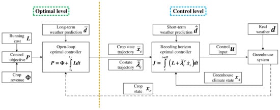
Figure 1.
Closed-loop optimal control of greenhouse climate based on two-time-scale decomposition.
The open-loop optimal control is solved with the control objective of maximizing the profit as shown in Equation (6). is the start of the growing period and specified to be 0 s. As the growing period is 50 days, is specified to be 4.32 × 10⁶ s. Long-term weather prediction is taken from the smoothed weather data. The method of quasi-steady state is used to reduce the computation load. This method assumes the greenhouse climate state to be static, which means in Equations (2)–(4). Then, the greenhouse climate state , the long-term weather prediction , the bounds on greenhouse climate as shown in Table 3, and the bounds on control inputs as shown in Table 2 are expressed in algebraic form in the lettuce growth model as shown in Equation (1). Details of the quasi-steady state computations are shown in [28]. In this way, the number of states in the greenhouse system model is reduced to 1, which is the lettuce state . Then, the pseudo-spectral algorithm is used to solve the open-loop optimal control problem with the software Tomlab. To increase the computing speed, the greenhouse system state and the control input should be scaled so that their maximal value equals 1. In addition, the number of collocation points should be gradually increased to 600. Since the growing period is 50 days, on average there is one collocation point each 2 h. The average sampling interval of 2 h in 50 days cannot be shorter in the current simulations because the computation load increases with the number of collocation points. On the other hand, the maximum number of collocation points in Tomlab is 608 [29].
In the method of two-time-scale decomposition [3], the crop state trajectory and the costate trajectory computed from the “optimal-level” are transferred to the “control-level” as parts of the control objective as shown in Equation (7). Optimal control at the “control-level” only concerns the greenhouse climate model as shown in Equations (2)–(4). In this way, the optimal control of the whole problem is decomposed into a slow subproblem dealing with crop dynamics at the slow time-scale and a fast subproblem dealing with greenhouse climate dynamics at the fast time-scale. In closed-loop simulations, the fast subproblem is repeatedly solved with the measured data.
Due to unavoidable model deficiencies and sensor errors, the optimal control algorithm is usually implemented in a closed-loop form. Receding horizon optimal control (RHOC) is used in this research with the control horizon being 1 h. The method of “lazy-man” is used for the short-term weather prediction [18]. The update interval of the receding horizon optimal controller is set to 10 min to match the variance frequency of the external weather in China. A longer update interval will lead to heavier greenhouse climate bound (shown in Table 3) violations due to short-term weather prediction errors. Moreover, the profit losses due to these violations are difficult to quantify in the control objective (6). That is also why these bounds are treated as hard constraints in the optimal control algorithm. The sampling interval of the control input in the control horizon is set to 20 min to increase the sensitivity of the control objective to control inputs in the first sampling interval [30].
Since the control inputs in this closed-loop optimal controller are piecewise constant, optimal control in this controller is first solved quickly with the pseudo-spectral algorithm in Tomlab. Then, the results are further improved in a digital optimal control algorithm that uses a nonlinear dynamic programming function “fmincon” in Matlab. This speeds up the solving of the digital optimal control problem [31]. Since the technology of online feedback of the crop state is not matured [32], this paper will not research the strategy of double-closed-loop optimal control [20]. The flow chart of the optimal control algorithm is shown in Figure 2. The computation time is considered in this research so that the closed-loop optimal control algorithm is closer to real implementations. When the computation time of the pseudo-spectral algorithm and the digital optimal control algorithm is within 10 min, the time delay of implementing the control equals the computation time. When the computation time is over 10 min, control inputs remain the same as those at the previous update instant. The investigation of computation time was performed on a commercial PC (CPU: i5-10500 @3.1 GHz, RAM: 8 GB).
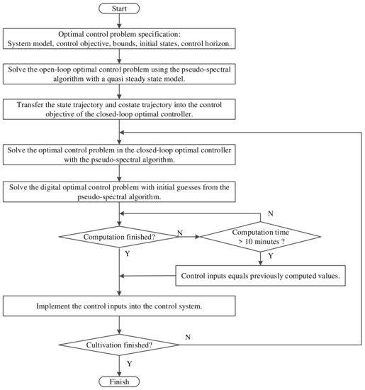
Figure 2.
Flow chart of the optimal control algorithm.
3. Results and Discussion
3.1. External Weather
The external weather data in Lhasa were collected every 10 min during the first 50 days of the year 2022, as shown in Figure 3. Note that in open-loop simulations the weather data are smoothed at each 2 h to cut down on computation load, while in closed-loop simulations the weather data are those collected every 10 min. From boxplots of the external weather, we can see that the selected period is cold (with a median of −2.7 °C for temperature) and dry (with a median of 25.2% for relative humidity). The solar radiation during the day can be as high as 1154 W m−2, although the median is 0 W m−2 because the dark period is longer than the light period.
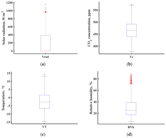
Figure 3.
External weather in Lhasa. (a) External solar radiation, (b) External CO2 concentration, (c) External temperature, (d) External relative humidity.
The growing period of lettuce grown in a greenhouse without LED lighting can last for 40 to 60 days. In winter the lettuce’s growing period can be up to 60 days, but in an optimally controlled greenhouse the lettuce can grow faster [24]. Therefore, 50 days of data were chosen to simulate the optimally controlled greenhouse in winter. The selected period covers the coldest days in Lhasa when the highest energy is spent on heating. Verification during this period is a guarantee of feasibility for the rest of the year. The choice of 50 days matches the reality of lettuce growth and is also adopted in relevant simulation research [19,20,24,27,28].
3.2. Open-Loop Simulations
Based on the order-reduced model through the method of quasi-steady state, open-loop optimal control is solved with the pseudo-spectral algorithm. Only the crop state trajectory and the costate trajectory are used in the control objective of the closed-loop optimal controller, as shown in Figure 2. The crop state trajectory and costate trajectory are shown in Figure 4. The costate trajectory represents the sensitivity of the control objective in the open-loop optimal control to the lettuce state . We can see that the costate is very high in the beginning and gradually increases in the later stage. This indicates that the increase in lettuce state in the early stage is very important for the profit of the whole growing period. The slow increase in the latter part indicates that it is gradually becoming more important to increase the lettuce state for a higher profit.
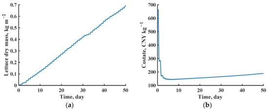
Figure 4.
Crop state trajectory and costate trajectory. (a) Crop state trajectory, (b) Costate trajectory.
The yield and profit indicators obtained from open-loop simulations are 14.49 kg [FW] m−2 and 13.72 CNY m−2 respectively. One should note that these indicators are obtained with the assumption that the model perfectly describes the behavior of the greenhouse–lettuce system. However, due to the performance loss caused by a shorter control horizon and short-term weather prediction errors in the closed-loop simulations, these indicators might be too idealistic and need to be corrected through closed-loop simulations. In closed-loop simulations, the performance loss caused by shorter sampling intervals, short-term weather predictions, and the computation time will be considered.
3.3. Closed-Loop Simulations
The closed-loop simulations involving the time delay caused by the computation process of nonlinear dynamic programming are performed over the whole growing period. The unavoidable shorter control horizon and the use of “lazy-man” short-term weather predictions lead to certain performance losses in the closed-loop simulations because of inadequate capture of the climate dynamics [19]. The inadequate capture of the climate dynamics leads to the difference between measured and computed states. Then the feedback in the closed-loop algorithm helps to correct the difference. Control inputs and the greenhouse climate during 2 days are shown in Figure 5 and Figure 6. We can see that all control inputs and the greenhouse climate are within their upper and lower bounds as shown in Table 2 and Table 3.
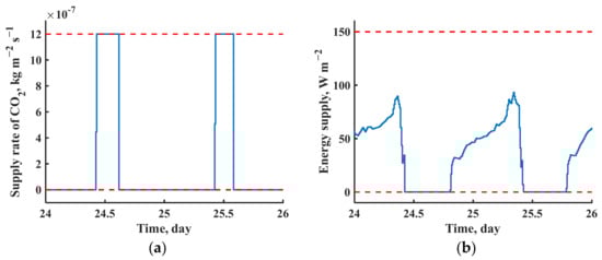
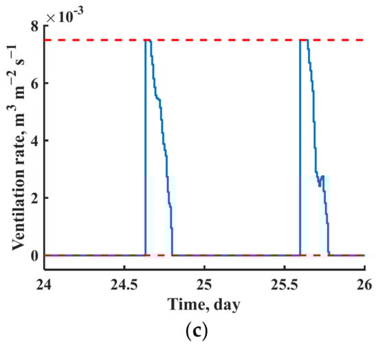
Figure 5.
Control inputs during 2 days. (a) Supply rate of CO2, (b) Energy supply, (c) Ventilation rate.
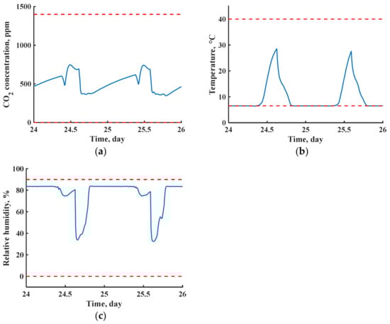
Figure 6.
Greenhouse climate during 2 days. (a) Internal CO2 concentration, (b) Internal temperature, (c) Internal relative humidity.
We can also see from Figure 5 that CO2 is usually supplied more as the solar radiation is higher. However, ventilation also happens during the day to lower the internal temperature. As a result, CO2 concentration is far from its upper bound, as shown in Figure 6. This is a trade-off between costs associated with prices. Because of the low external temperature and high solar radiation, the optimal controls in Lhasa are quite different from those in the Netherlands [19]. It is better to make use of cooling devices that can keep CO2 concentration at a higher level for better crop growth, such as the heat pump, but the feasibility of introducing such high-cost devices needs to be further researched. One may wonder why the maximum energy supply is close to midday as shown in Figure 5. This is relevant to the external temperature during these 2 days as shown in Figure 7.
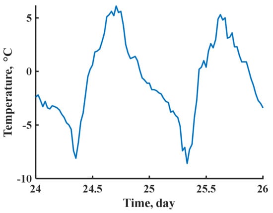
Figure 7.
External temperature during 2 days.
Numbers in closed-loop simulations without and with the computation time (denoted as RHOC and RHOCt) are shown in Table 4. When comparing the yield and profit in RHOC of Table 4 with their indicators in the open-loop simulations as shown in Section 3.2, we can see that they are all corrected to be lower (2.38 kg [FW] m−2 in yield, 11.01 CNY m−2 in profit). These corrections are consequences of the short-term weather prediction errors, the inadequate capture of climate dynamics due to a shorter control horizon, and the stricter satisfactions of greenhouse climate bounds due to a shorter sampling interval.
Table 4.
Numbers in closed-loop simulations without and with the computation time.
Closed-loop simulations seldom consider the time delay caused by the computation time of nonlinear dynamic programming in the receding horizon optimal controller, but the performance loss caused by the computation time is unavoidable. We can see from Table 4 that the yield and profit are further corrected to be lower (0.1 kg [FW] m−2 in yield, 0.87 CNY m−2 in profit) if we compare their numbers in RHOC and RHOCt. Although these corrections are not very high, they provide more realistic indicators for investors to make decisions. Moreover, the algorithm can be implemented in a real optimal controller because the computation time is unavoidable. One can see that the changes in CO2 cost and energy cost are very little, but the time delay leads to a slower response of the control system to the climate dynamics. This leads to a decrease in the actual yield and a resultant decrease in profit. One reason for the relatively sensitive response of the optimal control to the latency is that the crop model is sensitive to the climate. Another reason is that the latency leads to more effort to satisfy the greenhouse climate bounds in the closed-loop simulations. One should note that the profit is computed from the control objective in Equation (6) with local prices.
Growing lettuce in a heated and CO2-dosed Venlo greenhouse seems unprofitable when involving the fixed costs associated with the rent, labour, fertilizers, seeds, etc. However, we should keep in mind that the selected period covers the coldest days that cost the highest energy for heating. It can be expected that the profit can be higher during one cultivation period in the rest of the year. Further exploitation of the abundant solar energy in Lhasa can be investigated with the low-cost active solar water wall [33,34,35]. According to Xu etc. [34], the active solar water wall releases on average 22.6 W m−2 heat in Beijing daily. With stronger solar radiation in Lhasa, more than 27.12 kWh m−2 energy can be saved for heating for 50 days. This accounts for 47.49 CNY m−2 based on the energy price of 1.75 ¥ kWh−1 in Lhasa. As a result, the profit can be increased to 49.30 CNY m−2 according to Table 4. Moreover, the obtained profit represents the lowest level during the year because of the higher energy cost for heating in winter. For the rest of the year, a higher profit might compensate for the winter heating costs of greenhouse cultivation in Lhasa. The use of Chinese solar greenhouses might also help to cut down on energy costs [14]. However, dynamic modelling of the Chinese solar greenhouse climate should be validated before implementing the optimal control algorithm.
3.4. Summary of Time
As this paper deals with different time-scales and the computation time, a summary of different durations of time is shown in Table 5. The growing period of 50 days was fixed in this research because scheduling arrangements concerning the delivery of lettuce to sellers or customers generally demand a fixed harvest time [30]. The 2 h sampling interval of the weather data in open-loop simulations was smoothed from the collected weather data to cut down on computation load [27]. The 1 h horizon of “lazy-man” weather prediction equals the control horizon in closed-loop simulations, and this is decided by the performance loss through research [18]. The 20 min sampling interval of controls is longer than the 10 min update interval to increase the sensitivity of performance to controls in the update interval [29]. The update interval of control inputs is related to the varying frequency of the external weather [29]. The longest computation time is within the update interval of 10 min. If the time delay caused by the computation time is longer than the update interval, the algorithm will keep the control inputs as previously computed until the current computation finishes as shown in Figure 2.
Table 5.
Different durations of time.
Although the computation time seems trivial compared with the update interval, it grows drastically with the increase in the number of model states or control inputs [20]. Therefore, it is important to quantify the influence of computation time before cultivation. One should note that the uncertainties in the model can be handled by an adaptive optimal controller [28] and this will further increase the computation time. However, this is out of the scope of this paper and will be researched in the future with real implementations.
4. Conclusions
- Open-loop simulations of the optimal control of greenhouse lettuce cultivation in Lhasa generate yield and profit indicators of 14.49 kg m−2 and 13.72 CNY m−2, respectively. In closed-loop simulations, these indicators are corrected to 2.38 kg m−2 and 11.01 CNY m−2 lower, respectively, because of short-term weather prediction errors and a shorter sampling interval than that in the open-loop. When the computation time of the nonlinear dynamic programming is considered, further corrections in yield and profit indicators from closed-loop simulations can be up to 0.1 kg m−2 and 0.87 CNY m−2, respectively. These indicators are closer to real implementations and can help investors make wiser decisions before cultivation.
- Due to the low temperature and high solar radiation in Lhasa, a mix of simultaneous ventilation and CO2 supply occurs as a trade-off between costs associated with prices. As a result, the CO2 concentration is far from its upper bound although the CO2 supply is maximum at noon. Although the external temperature is low, ventilation is needed at noon for reducing the internal temperature because of the high solar radiation.
- The profit in optimal control of Venlo greenhouse lettuce cultivation can be as low as 1.84 CNY m−2 on the coldest days in Lhasa. However, if the abundant solar energy in Lhasa can be further exploited, such as with an active solar water wall, the profit can be increased to more than 49.30 CNY m−2. For future applications, low-cost solar-heating devices should be modelled and incorporated into the optimal control algorithm to increase profit and sustainability.
Author Contributions
Conceptualization, D.X., S.Z., and W.S.; methodology, D.X.; resources, Y.L., A.D.; writing—original draft preparation, D.X.; writing—review and editing, D.X., S.Z., and W.S. All authors have read and agreed to the published version of the manuscript.
Funding
This work was financially supported by the National Natural Science Foundation of China (U20A2020), Key Technology Research and Development Program of Shandong (2022CXGC020708), National Modern Agricultural Technology System Construction Project (CARS-23-C02), and Beijing Innovation Consortium of Agriculture Research System (BAIC01-2022).
Informed Consent Statement
Not applicable.
Data Availability Statement
Not applicable.
Conflicts of Interest
The authors declare no conflict of interest.
References
- Van Straten, G.; Van Willigenburg, L.G.; Van Henten, E.J.; Van Ooteghem, R.J.C. Optimal Control of Greenhouse Cultivation; CRC Press: Boca Raton, FL, USA, 2011. [Google Scholar]
- Singhal, R.; Kumar, R.; Neeli, S. Receding horizon control based on prioritised multi-operational ranges for greenhouse environment regulation. Comput. Electron. Agric. 2021, 180, 105840. [Google Scholar] [CrossRef]
- Van Henten, E.J.; Bontsema, J. Time-scale decomposition of an optimal control problem in greenhouse climate management. Control. Eng. Pract. 2009, 17, 88–96. [Google Scholar] [CrossRef]
- Liu, T.; Yuan, Q.; Wang, Y. Hierarchical optimization control based on crop growth model for greenhouse light environment. Comput. Electron. Agric. 2021, 180, 105854. [Google Scholar] [CrossRef]
- Kuijpers, W.J.; Antunes, D.J.; Van Mourik, S.; Van Henten, E.J.; Van De Molengraft, M.J. Weather forecast error modelling and performance analysis of automatic greenhouse climate control. Biosyst. Eng. 2022, 214, 207–229. [Google Scholar] [CrossRef]
- Katzin, D.; Van Henten, E.J.; Van Mourik, S. Process-based greenhouse climate models: Genealogy, current status, and future directions. Agric. Syst. 2022, 198, 103388. [Google Scholar] [CrossRef]
- Van Beveren, P.J.M.; Bontsema, J.; Van’t Ooster, A.; Van Straten, G.; Van Henten, E.J. Optimal utilization of energy equipment in a semi-closed greenhouse. Comput. Electron. Agric. 2020, 179, 105800. [Google Scholar] [CrossRef]
- Lin, D.; Zhang, L.; Xia, X. Model predictive control of a Venlo-type greenhouse system considering electrical energy, water and carbon dioxide consumption. Appl. Energy 2021, 298, 117163. [Google Scholar] [CrossRef]
- Seginer, I.; Van Straten, G.; Van Beveren, P.J.M. Day-to-night heat storage in greenhouses: 4. Changing the environmental bounds. Biosyst. Eng. 2020, 192, 90–107. [Google Scholar] [CrossRef]
- González, R.; Rodriguez, F.; Guzmán, J.L.; Berenguel, M. Robust constrained economic receding horizon control applied to the two time—Scale dynamics problem of a greenhouse. Optim. Control. Appl. Methods 2014, 35, 435–453. [Google Scholar] [CrossRef]
- Achour, Y.; Ouammi, A.; Zejli, D.; Sayadi, S. Supervisory model predictive control for optimal operation of a greenhouse indoor environment coping with food-energy-water Nexus. IEEE Access 2020, 8, 211562–211575. [Google Scholar] [CrossRef]
- Lin, D.; Zhang, L.; Xia, X. Hierarchical model predictive control of Venlo-type greenhouse climate for improving energy efficiency and reducing operating cost. J. Clean. Prod. 2020, 264, 121513. [Google Scholar] [CrossRef]
- Bersani, C.; Fossa, M.; Priarone, A.; Sacile, R.; Zero, E. Model Predictive Control versus Traditional Relay Control in a High Energy Efficiency Greenhouse. Energies 2021, 14, 3353. [Google Scholar] [CrossRef]
- Hu, G.; You, F. Model predictive control for greenhouse condition adjustment and crop production prediction. Comput. Aided Chem. Eng. 2022, 51, 1051–1056. [Google Scholar]
- Ren, Z.; Dong, Y.; Lin, D.; Zhang, L.; Fan, Y.; Xia, X. Managing energy-water-carbon-food nexus for cleaner agricultural greenhouse production: A control system approach. Sci. Total Environ. 2022, 848, 157756. [Google Scholar] [CrossRef]
- Chen, W.H.; Mattson, N.S.; You, F. Intelligent control and energy optimization in controlled environment agriculture via nonlinear model predictive control of semi-closed greenhouse. Appl. Energy 2022, 320, 119334. [Google Scholar] [CrossRef]
- Su, Y.; Xu, L.; Goodman, E.D. Multi-layer hierarchical optimisation of greenhouse climate setpoints for energy conservation and improvement of crop yield. Biosyst. Eng. 2021, 205, 212–233. [Google Scholar] [CrossRef]
- Tap, R.F. Economics-Based Optimal Control of Greenhouse Tomato Crop Production. Ph.D. Thesis, Wageningen University, Wageningen, The Netherlands, 2000. [Google Scholar]
- Xu, D.; Du, S.; Van Willigenburg, L.G. Optimal control of Chinese solar greenhouse cultivation. Biosyst. Eng. 2018, 171, 205–219. [Google Scholar] [CrossRef]
- Xu, D.; Du, S.; Van Willigenburg, L.G. Double closed-loop optimal control of greenhouse cultivation. Control. Eng. Pract. 2019, 85, 90–99. [Google Scholar] [CrossRef]
- Li, E.; Zhu, J. Parametric analysis of the mechanism of creating indoor thermal environment in traditional houses in Lhasa. Build. Environ. 2022, 207, 108510. [Google Scholar] [CrossRef]
- Ioslovich, I.; Gutman, P.O.; Linker, R. Hamilton–Jacobi–Bellman formalism for optimal climate control of greenhouse crop. Automatica 2009, 45, 1227–1231. [Google Scholar] [CrossRef]
- Righini, I.; Vanthoor, B.; Verheul, M.J.; Naseer, M.; Maessen, H.; Persson, T.; Stanghellini, C. A greenhouse climate-yield model focussing on additional light, heat harvesting and its validation. Biosyst. Eng. 2020, 194, 1–15. [Google Scholar] [CrossRef]
- Van Henten, E.J. Greenhouse Climate Management: An Optimal Control Approach. Ph.D. Thesis, Wageningen University, Wageningen, The Netherlands, 1994. [Google Scholar]
- Van Ooteghem, R.J.C. Optimal Control Design for a Solar Greenhouse. Ph.D. Thesis, Wageningen University, Wageningen, The Netherlands, 2007. [Google Scholar]
- Vanthoor, B.H.E. A Model-Based Greenhouse Design Method. Ph.D. Thesis, Wageningen University, Wageningen, The Netherlands, 2011. [Google Scholar]
- Van Henten, E.J. Sensitivity analysis of an optimal control problem in greenhouse climate management. Biosyst. Eng. 2003, 85, 355–364. [Google Scholar] [CrossRef]
- Xu, D.; Du, S.; Van Willigenburg, L.G. Adaptive two time-scale receding horizon optimal control for greenhouse lettuce cultivation. Comput. Electron. Agric. 2018, 146, 93–103. [Google Scholar] [CrossRef]
- Rutquist, P.E.; Edvall, M.M. Propt-Matlab Optimal Control Software; Tomlab Optimization Inc.: Washington, DC, USA, 2010. [Google Scholar]
- Van Willigenburg, L.G.; Van Henten, E.J.; Van Meurs, W.T.M. Three time-scale digital optimal receding horizon control of the climate in a greenhouse with a heat storage tank. IFAC Proc. Vol. 2000, 33, 149–154. [Google Scholar] [CrossRef]
- Xu, D.; Ahmed, H.A.; Tong, Y.; Yang, Q.; Van Willigenburg, L.G. Optimal control as a tool to investigate the profitability of a Chinese plant factory—Lettuce production system. Biosyst. Eng. 2021, 208, 319–332. [Google Scholar] [CrossRef]
- Van Beveren, P.J.M.; Bontsema, J.; Van Straten, G.; Van Henten, E.J. Optimal control of greenhouse climate using minimal energy and grower defined bounds. Appl. Energy 2015, 159, 509–519. [Google Scholar] [CrossRef]
- Xu, W.; Song, W.; Ma, C. Performance of a water-circulating solar heat collection and release system for greenhouse heating using an indoor collector constructed of hollow polycarbonate sheets. J. Clean. Prod. 2020, 253, 119918. [Google Scholar] [CrossRef]
- Xu, W.; Guo, H.; Ma, C. An active solar water wall for passive solar greenhouse heating. Appl. Energy 2022, 308, 118270. [Google Scholar] [CrossRef]
- Wang, J.; Qu, M.; Zhao, S.; Ma, C.; Song, W. New insights into the scientific configuration of a sheet heating system applied in Chinese solar greenhouse. Appl. Therm. Eng. 2023, 219, 119448. [Google Scholar] [CrossRef]
Disclaimer/Publisher’s Note: The statements, opinions and data contained in all publications are solely those of the individual author(s) and contributor(s) and not of MDPI and/or the editor(s). MDPI and/or the editor(s) disclaim responsibility for any injury to people or property resulting from any ideas, methods, instructions or products referred to in the content. |
© 2022 by the authors. Licensee MDPI, Basel, Switzerland. This article is an open access article distributed under the terms and conditions of the Creative Commons Attribution (CC BY) license (https://creativecommons.org/licenses/by/4.0/).