Article

Predicting Sugarcane Biometric Parameters by UAV Multispectral Images and Machine Learning

by
Romário Porto de Oliveira
*,
Marcelo Rodrigues Barbosa Júnior
,
Antônio Alves Pinto
,
Jean Lucas Pereira Oliveira
,
Cristiano Zerbato
and
Carlos Eduardo Angeli Furlani
Department of Engineering and Exact Sciences, School of Veterinarian and Agricultural Sciences, São Paulo State University (Unesp), Jaboticabal 14884-900, SP, Brazil
*
Author to whom correspondence should be addressed.
Agronomy 2022, 12(9), 1992; https://doi.org/10.3390/agronomy12091992
Submission received: 5 July 2022 / Revised: 12 August 2022 / Accepted: 18 August 2022 / Published: 23 August 2022

Abstract

:
Multispectral sensors onboard unmanned aerial vehicles (UAV) have proven accurate and fast to predict sugarcane yield. However, challenges to a reliable approach still exist. In this study, we propose to predict sugarcane biometric parameters by using machine learning (ML) algorithms and multitemporal data through the analysis of multispectral images from UAV onboard sensors. The research was conducted on five varieties of sugarcane, as a way to make a robust approach. Multispectral images were collected every 40 days and the evaluated biometric parameters were: number of tillers (NT), plant height (PH), and stalk diameter (SD). Two ML models were used: multiple linear regression (MLR) and random forest (RF). The results showed that models for predicting sugarcane NT, PH, and SD using time series and ML algorithms had accurate and precise predictions. Blue, Green, and NIR spectral bands provided the best performance in predicting sugarcane biometric attributes. These findings expand the possibilities for using multispectral UAV imagery in predicting sugarcane yield, particularly by including biophysical parameters.

1. Introduction

Sugarcane is a semi-perennial grass grown globally, mainly in tropical and subtropical countries, represented as a product of great importance for international agricultural trade and relevant raw material for agroindustry [1]. It can massively produce sugar, biofuel, and biopower [2]. Hence, timely and accurate sugarcane yield prediction is valuable for national food security and sustainable agriculture development [3]. Predicting sugarcane yield is not an easy task and, although previous studies have found solutions to this puzzle, challenges still need to be addressed. Thereby, the development of an alternative is necessary.
Reviewing in-depth the academic literature on sugarcane yield prediction, we can find several studies on remote sensing solutions. For instance, a satellite approach by Abebe, Tadesse, and Gessesse [4], combined Landsat 8 and Sentinel 2A imagery for improved sugarcane yield estimation. The approach applied the most popular vegetation indices (VIs) for the second and third ratoon sugarcane crop and used support vector regression (SVR) as a statistical method. Their results were useful for sugarcane yield estimation. Nevertheless, crop yield depends on soil type, weather conditions, plant genotype, and management practices. Hence, the use of a single type of observation is not reliable to provide the true state of the agroecological system, causing misinformation about crop yield estimation [5]. Another contribution by Yu et al. [6], highlights the simulations by integrating multi-source observations in sugarcane fields. Stronger points in this study included PH, leaf area index, and soil moisture variables to improve reliable sugarcane yield estimation. Collaboration is timely and provides an improvement in academic progress. However, uncertainties and limitations have been noted, mainly in the statistical model to characterize the potential growth of PH, which constrains further applications. By further analyzing the bibliographic collection, we can examine another important collaboration by Tanut, Waranusast, and Riyamongkol [7]. They used a new generation of remote sensing platforms, the UAV. Here, the authors [7], proposed high accuracy by using data mining and reverse design methods. Data of various variables were used, such as sugarcane variety, plant distance, ratoon cut count, yield level, and soil group. The results for sugarcane yield prediction were reached with an accuracy of 98.69% but are still limited since they only used RGB images.
The canopy density of the sugarcane plantation is challenging to map, resulting in increased difficulties in yield estimation. These issues often result in less accurate and unreliable yield estimations. NT, PH, and SD have a large influence on the final sugarcane yield, as they are agronomic traits which are widely used to estimate yield [8,9,10,11,12]. Sugarcane yield is characterized by approximately 70% contribution by the NT, 27% by PH, and 3% by SD [13]. However, mainly NT and SD are still quantified by counting in the field, a laborious and time-consuming task. Therefore, a new further approach is necessary, and UAVs prove to be useful for it. On the other hand, traditional statistic methods assume linear correlations between observed and predict yields, which could not accurately reflect non-linear relationships. Thus, ML algorithms can be adopted to overcome these challenges [14]. Random forest is a decision tree ML algorithm with great potential in agronomic predictions, such as yield prediction [15], and biomass estimation [16]. Another widely applied algorithm is the MLR. It is a low-complexity regression model and has found reliable prediction results in previous studies [4,17,18,19].
In this work, we propose to expand the possibilities of sugarcane yield prediction, mainly by including data from biophysical parameters obtained by remote sensing. Therefore, we analyzed how RF and MLR models can address the puzzle of predicting NT, PH, and SD using UAV multispectral images in search for timely results in remote sugarcane yield prediction, thus being able to improve sugarcane yield prediction.

2. Material and Methods

2.1. Site of Study and Biometric Data

The study was conducted in an experimental field located at the São Paulo State University, Jaboticabal, São Paulo, Brazil (21°14′57″ S, 48°16′55″ W, and altitude of ~570 m). The local climate is Cwa, a humid subtropical climate with a dry winter season and an average annual temperature of 22 °C [20]. The rainy season is concentrated between November and March, with an annual average of 1428 mm. The soil type is Oxisol [21].
Five sugarcane cultivars were planted in the experimental area, namely CTC4, CTC9001, IACSP95-5094, RB867515, and RB966928. All cultivars formed a single plant group to increase the robustness of this approach. We collected data from 240 plant rows (48 plant rows per cultivar). The plant rows corresponded to 10 m in length. We counted the NT of all plants in the row and then converted it to NT m−1. We used the average value of ten plants measured in the row for SD and PH. NT and PH were measured at 130 days after planting (DAP), a period near the end of tillering [22,23], and SD was measured at 220 DAP (Figure 1). Growing degree days (GDD) corresponding to the data collection period were determined to establish relationships between canopy spectral changes and production components (Figure 1).

2.2. UAV-Based Data Collection

We carried out three flights at 80, 120, and 160 DAP (Figure 1). We used a multispectral camera (MicaSense RedEdge-M, MicaSense Inc., Seattle, WA, USA) onboard a multirotor UAV for flight. The sensor captures five spectral bands: Blue, Green, Red, RedEdge, and NIR (Table 1). The flights were performed at a 30 m altitude, thus ensuring a ground sample distance (GSD) of 2.8 cm. We adopted an overlap of 75% front and 70% side. Images were stitched using SfM software (Agisoft Metashape Professional 1.5.5, Agisoft, St. Petersburg, Russia). We segmented the orthomosaics before applying the proposed approach to remove the interference from the soil background. Finally, spectral band information and VIs (Table 2) were obtained by using the Mask and Zonal Statistical tools from QGIS 3.10.9 software (Free software Inc., Boston, MA, USA).

2.3. Predict on ML

2.3.1. Data Curation

A functional dataset was generated to group the data (Figure 2). The spectral data corresponding to each image collection date were evaluated separately and together to determine which one performs best in predicting the parameters. The independent variables used in the models were spectral bands (Table 1) and three VIs (Table 2). The biometric parameters of sugarcane measured in the field consisted of dependent variables. We used the Z-score method to detect and remove outliers from the dataset [27]. The stepwise analysis was performed using the RF algorithm to select the best independent variables to be used in the prediction models. This method determines the variables that have the greatest influence on the result set. Thus, we used only those that provide the greatest efficiency in the model. The root mean square error (RMSE) was the metric used to select the best performing predictor variables by stepwise.

2.3.2. Data Analysis

In this paper, we used two ML prediction models, namely MLR and RF. The models were processed using the open-source ML library ‘scikit-learn’ in Python programming language v3.8.10 in the Jupyter Notebook environment. We selected the best combination of the number of trees (n_estimators) and maximum tree depth (max_depth) for RF. The validation method “K-fold cross-validation” was used. This validation method was applied with K = 5. The dataset was divided into five subsets (fold), in which 80% of the data was used for training and 20% for validation. We repeated the process 5 times, and the model was trained and validated on different datasets in each repetition. The performance of the MLR and RF models was evaluated by considering the coefficient of determination (R2), mean absolute error (MAE), and root mean square error (RMSE). Figure 2 shows an overview of the methodology.

3. Results

3.1. Selection of Predictor Variables

We obtained two predictor combinations with good performance composed of two and three variables. The first selected combination composed of two variables was represented by the Blue and Green spectral bands, while the second combination corresponded to the Blue, Green, and NIR bands. The combination of two and three variables was similar for NT, with RMSE = 3.9 and 3.6, respectively. We noted that performance was stable using two to six variables (Figure 3a). The same was observed for SD (Figure 3c). Thus, using one variable or more than six increases the error. The predictor variables for SD showed RMSE = 2.54 mm and 2.52 mm for two and three variables, respectively. Different results were found for PH. The numbers of variables showed similar results, with quickly better results for two (RMSE = 20.4 cm) and three variables (RMSE = 20.2 cm). Thus, models were tested using the two selected combinations of variables, with two and three variables, as all bands in the first combination (two variables) are in the visible spectral region.

3.2. Predictions of Biometric Parameters

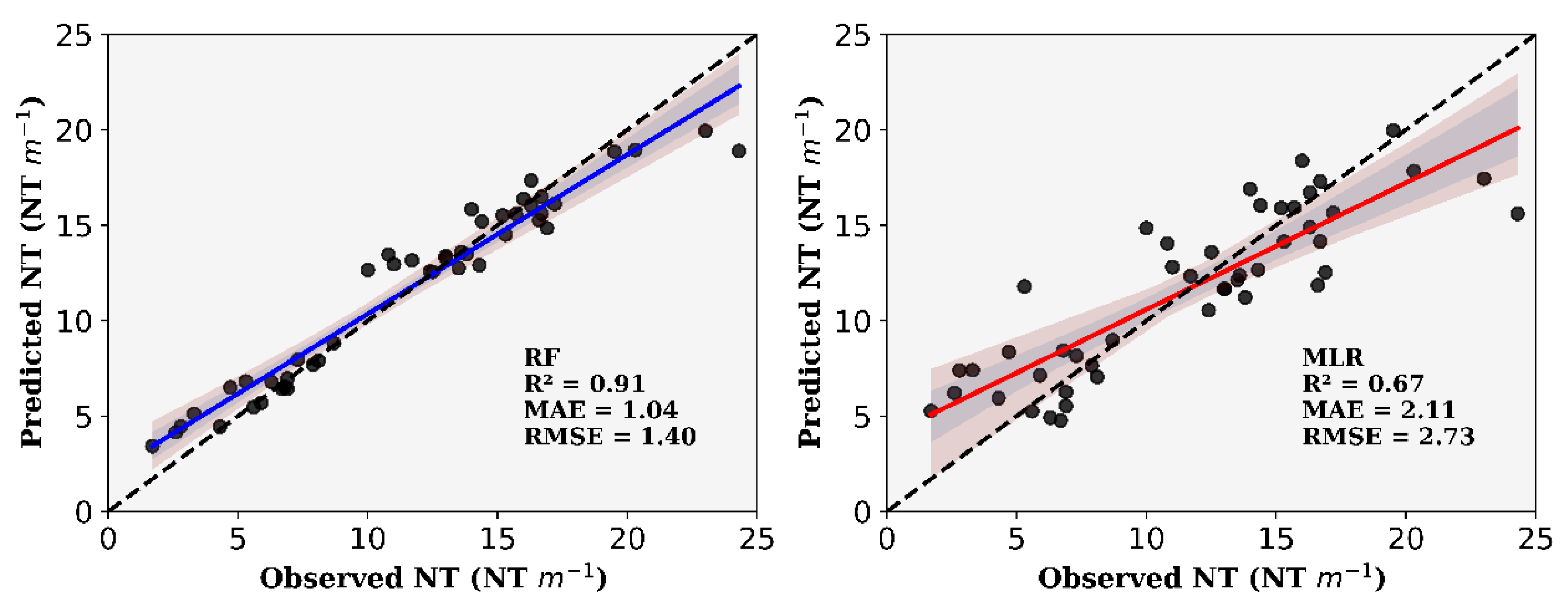
3.2.1. Predicting the Number of Tillers

The best prediction models for NT were reached using the RF algorithm with three variables (Table 3). The fusion of image time series data (GDD = 349 + 397) provided better precision and accuracy using three variables, with R2 = 0.91, MAE = 1.04, and RMSE = 1.40. In contrast, for independent predictions, the images collected at 349 GDD showed better precision and accuracy (higher R2 and lower MAE and RMSE) compared to 397 GDD. We clearly observed that model accuracy or precision decreased for predictions using two variables. The results were also similar to those found for models with three variables, in which the combination of GDDs ensured better performance than independent prediction (R2 = 0.88, MAE = 1.29, and RMSE = 1.67). Moreover, the images collected at a GDD of 349 also showed better performance for independent prediction (R2 = 0.85, MAE = 1.42, and RMSE = 1.83).
Predictions of NT using the MLR algorithm presented similar results to RF, but with lower precision and accuracy values (Table 3). Model precision and accuracy using three variables outperformed models with two variables. The combination of GDD = 349 and 397 showed a slightly higher precision and accuracy with three variables than the independent prediction of 349 GDD (R2 = 0.67 to 0.65, MAE = 2.11 to 2.16, and RMSE = 2.73 to 2.78, respectively). This pattern of better models was sustained when we used two variables, and again the combination of GDDs provided better results. The best correlations between observed and predicted NT are shown in Figure 4.

3.2.2. Predicting Plant Height

The RF algorithm outperformed the MLR regarding the result of PH prediction (Table 4). In addition, models using three variables performed better than those with two variables. Images corresponding to GDD = 349 and 397 revealed more precise and accurate results. The images collected at 349 GDD showed more precise and accurate results when considering only independent predictors. In contrast, the combination of GDD = 349 and 397 showed better performance for two variables than individual GDD values. However, we can reach reliable results if we still choose to use only the data at 349 GDD, for example (R2 = 0.81, MAE = 8.60 cm, and RMSE = 11.16 cm).
MLR-based models were not as efficient as RF. However, an accuracy >0.60 could be obtained when we used two and three variables (Table 4). Once again, models with three variables were more accurate and precise. Our results showed better fit for fusions of GDD = 349 and 397 (R2 = 0.60, MAE = 12.89 cm, and RMSE = 16.32 cm). Nevertheless, we can still achieve potential results for independent predictors, especially at 397 GDD (R2 = 0.53, MAE = 14.09 cm, and RMSE = 17.49 cm). The fit of the observed and predicted PH is shown in Figure 5.

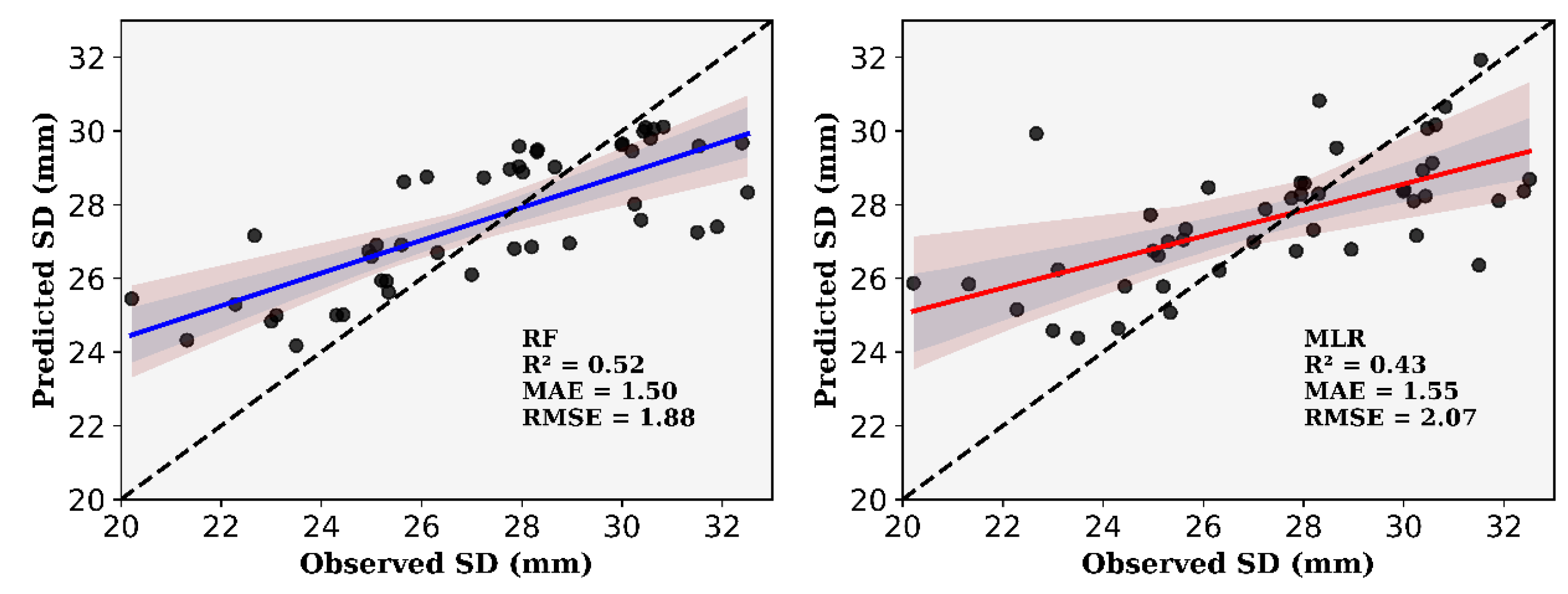
3.2.3. Predicting Stalk Diameter

Clearly, we can see that using three variables gave us better results, either for RF or MLR. But, in short, the prediction results for SD showed more accurate and precise models using the RF algorithm (Table 5). A particularity in the SD prediction was relative to the image collection periods. The fusion of data collected at 349 and 397 GDD allowed better results, similarly when we added the data from 410 GDD. Otherwise, if capturing images on a single date is the only option, we obtain better precision and accuracy at 349 GDD either for two or three variables (R2 = 0.49 to 0.51, MAE = 1.54 to 1.53 mm, and RMSE = 1.97 to 1.95 mm, respectively).
The application of the MLR algorithm to predict SD produced better results in the combination of images collected at 349, 397, and 410 GDD (R2 = 0.43, MAE = 1.55 mm, and RMSE = 2.07 mm). However, we had closely similar results when combining only data at 349 and 397 GDD (R2 = 0.40, MAE = 1.64 mm, and RMSE = 2.14 mm) (Table 5). Moreover, if we decide to use only one collection date, we can collect the data at 349 GDD and still have similar results (R2 = 0.38, MAE = 1.64 mm, and RMSE = 2.17 mm). In this prediction, lower precision and accuracy were reached at 397 GDD (R2 = 0.15, MAE = 1.75, and RMSE = 2.25 mm). Although using two variables is not the best option, considerable values can be achieved by fusing data from 349, 397, and 410 GDD (R2 = 0.36, MAE = 1.68 mm, and RMSE = 2.19 mm). Better metrics for independent prediction of SD were found at 349 GDD (R2 = 0.35, MAE = 1.72 mm, and RMSE = 2.22 mm). In summary, RF and MLR models can predict SD with high accuracy, but with low precision (Figure 6).

4. Discussion

In this study, we analyzed whether multispectral UAV images can predict the biophysical parameters of sugarcane, mainly the NT, PH, and SD. If confirmed, it could serve as a timely basis for accurately predicting sugarcane yield. We can find several studies that investigated improvements in sugarcane yield prediction [4,6,7], but to the best of our knowledge, this is the first approach that has used multispectral UAV images combining ML algorithms to predict the NT, PH, and SD, three essential parameters for predicting sugarcane yield [10,11,12].
The stepwise method applied in our approach presented the Blue, Green, and NIR bands as the best input predictors for predicting NT, PH, and SD of sugarcane. The stepwise selection of variables showed stability in the model accuracy. Thus, models composed with more than three variables showed no significant influence on model precision and accuracy, allowing simplification by reducing the input variables. The use of combined image data (time series) and uncombined image data (independent prediction—only data from one image) allowed us to obtain precise and accurate results to predict sugarcane biometric parameters. This information should be used for a better understanding of the variability in the field and, therefore, the decision making by producers.
The RF models performed better than MLR in predicting all parameters. High R2 values were achieved for NT and PH (R2 > 0.70). Previous studies also investigated RF and MLR algorithms to predict yield in crops such as wheat and potato [15]. The authors observed that RF models outperformed MLR models for all evaluated crops. The outperformance of RF is attributed to its particularity of correcting the overfitting decision habit to the training subset [28]. On the other hand, there is still the inability of MLR to process nonlinear relationships between dependent and independent variables [29].
Regarding the use of two or three input predictor variables, models with three variables presented more accurate and precise results, but with values close to models with two variables. Models with two variables used blue and green spectral bands. These bands are in the visible spectral range, which would be an alternative for users of RGB cameras, which typically have lower costs than multispectral cameras and require fewer calibration procedures [30,31]. Some studies on crop yield predictions have found similar results between vegetation indices calculated by the Blue, Green, and NIR bands [32,33]. In these studies, RF and linear regression models presented better results using the combination of these indices.
In our study, two (Blue and Green) and three (Blue, Green, and NIR) input variables presented good results to predict NT and the combination of 349 and 397 GDD provided the most accurate and precise results. These results can be related to the canopy reflectance characteristics, as leaf area index [34], and biomass [35], increase when NT increases. This growth in canopy coverage causes higher absorption of visible electromagnetic radiation due to the strong influence of leaf pigments [36,37]. In this case, the blue band is absorbed in greater proportion in plants with higher tillering rates because chlorophyll strongly absorbs radiation at wavelengths in the visible range [38]. The same process can be related to the Green band. However, this band is characterized by a lower radiation absorption compared to the Blue band, for example. On the other hand, it reflects less than the NIR band [36,37]. Sumesh et al. [35], used IV obtained from RGB images (excess green index—ExG) and ordinary least squares (OLS) regression to estimate sugarcane stalk density, obtaining R2 = 0.72 and RMSE = 9.84. NIR is a spectral band that reflects higher values in healthy plants, and the reflectance increases as the leaf area index increases. In this sense, good results including the NIR band in NT prediction may be strongly related to the high sensitivity of this band to variations in biomass [37,39,40]. Other studies on the estimation of sugarcane parameters by multispectral images have obtained good results using VIs derived from NIR and a visible spectrum band, such as NDVI [41,42].
Accurate prediction models were obtained for PH and SD. PH and SD are features that directly correlate with biomass [43,44,45]. In this regard, several studies have found relationships between spectral bands, VIs, and crop biophysical parameters, especially biomass, as these parameters influence the intensity of plant reflectance [16,45,46]. Although SD quickly showed lower precision (R2 = 0.43–0.52), we can still reliably predict sugarcane yield since NT and PH were highly precise. Parameters with SD are less representative in the prediction because higher biomass indices are mainly associated with NT and PH [10]. Overall, our results showed that models for predicting NT, PH, and SD of sugarcane through time series and MLR and RF algorithms presented accurate predictions. Therefore, the use of multispectral sensors on board UAVs can be considered a viable technique for evaluating sugarcane crops since it presents the ability to monitor large production areas with high spatial resolution. In further studies, we will apply this approach to different soil types and planting seasons.

5. Conclusions

Predicting sugarcane yield is an important task for planning and managing decisions, such as the harvesting schedule. In our approach, we used spectral bands obtained by a multispectral sensor on board a UAV associated with ML algorithms to predict sugarcane NT, PH, and SD. Answering our objectives, straightforward preliminary evidence exists for the exceptional ability to predict these parameters by UAV imagery. Therefore, we provide timely results in this study to improve sugarcane yield prediction. Models based on RF algorithms showed higher accuracy and precision than MLR models. Blue, Green, and NIR spectral bands provided good performance for predicting sugarcane biometric attributes. Moreover, the combination of images collected in more than one period further improves the model accuracy for predicting the biometric parameters. Therefore, this study demonstrates the effectiveness of using multispectral UAV images to build a model for estimating sugarcane yield.

Author Contributions

Conceptualization, R.P.d.O.; methodology, R.P.d.O. and C.Z.; formal analysis, R.P.d.O.; investigation, R.P.d.O., M.R.B.J., A.A.P. and J.L.P.O.; data curation, R.P.d.O.; writing—original draft, R.P.d.O.; writing—review and editing, R.P.d.O., A.A.P., C.E.A.F., M.R.B.J.; visualization, R.P.d.O., M.R.B.J., A.A.P., J.L.P.O., C.E.A.F. and C.Z.; supervision, C.E.A.F.; project administration, C.E.A.F. All authors have read and agreed to the published version of the manuscript.

Funding

This work was supported by Coordination for the Improvement of Higher Education Personnel (CAPES), Process No. 88887.512497/2020-00; and Coordination of the Graduate Program in Agronomy (Plant Production).

Acknowledgments

We would like to acknowledge the Laboratory of Machines and Agricultural Mechanization (LAMMA) of the Department of Engineering and Exact Sciences for the infrastructural support.

Conflicts of Interest

The authors declare no conflict of interest.

References

  1. FAOSTAT—Food and Agriculture Organization of the United Nation. Available online: http://www.fao.org/faostat/en/?#data/QC (accessed on 27 December 2021).
  2. Barbosa Júnior, M.R.; de Almeida Moreira, B.R.; de Brito Filho, A.L.; Tedesco, D.; Shiratsuchi, L.S.; da Silva, R.P. UAVs to Monitor and Manage Sugarcane: Integrative Review. Agronomy 2022, 12, 661. [Google Scholar] [CrossRef]
  3. Abebe, G.; Tadesse, T.; Gessesse, B. Assimilation of Leaf Area Index from Multisource Earth Observation Data into the WOFOST Model for Sugarcane Yield Estimation. Int. J. Remote Sens. 2022, 43, 698–720. [Google Scholar] [CrossRef]
  4. Abebe, G.; Tadesse, T.; Gessesse, B. Combined Use of Landsat 8 and Sentinel 2A Imagery for Improved Sugarcane Yield Estimation in Wonji-Shoa, Ethiopia. J. Indian Soc. Remote Sens. 2022, 50, 143–157. [Google Scholar] [CrossRef]
  5. Wang, J.; Li, X.; Lu, L.; Fang, F. Estimating near Future Regional Corn Yields by Integrating Multi-Source Observations into a Crop Growth Model. Eur. J. Agron. 2013, 49, 126–140. [Google Scholar] [CrossRef]
  6. Yu, D.; Zha, Y.; Shi, L.; Ye, H.; Zhang, Y. Improving Sugarcane Growth Simulations by Integrating Multi-Source Observations into a Crop Model. Eur. J. Agron. 2022, 132, 126410. [Google Scholar] [CrossRef]
  7. Tanut, B.; Waranusast, R.; Riyamongkol, P. High Accuracy Pre-Harvest Sugarcane Yield Forecasting Model Utilizing Drone Image Analysis, Data Mining, and Reverse Design Method. Agriculture 2021, 11, 682. [Google Scholar] [CrossRef]
  8. Som-ard, J.; Hossain, M.D.; Ninsawat, S.; Veerachitt, V. Pre-Harvest Sugarcane Yield Estimation Using UAV-Based RGB Images and Ground Observation. Sugar Tech. 2018, 20, 645–657. [Google Scholar] [CrossRef]
  9. Rossi Neto, J.; de Souza, Z.M.; Kölln, O.T.; Carvalho, J.L.N.; Ferreira, D.A.; Castioni, G.A.F.; Barbosa, L.C.; de Castro, S.G.Q.; Braunbeck, O.A.; Garside, A.L.; et al. The Arrangement and Spacing of Sugarcane Planting Influence Root Distribution and Crop Yield. Bioenergy Res. 2018, 11, 291–304. [Google Scholar] [CrossRef]
  10. Zhao, D.; Irey, M.; Laborde, C.; Hu, C.J. Identifying Physiological and Yield-Related Traits in Sugarcane and Energy Cane. Agron. J. 2017, 109, 927–937. [Google Scholar] [CrossRef]
  11. Zhao, D.; Irey, M.; Laborde, C.; Hu, C.J. Physiological and Yield Characteristics of 18 Sugarcane Genotypes Grown on a Sand Soil. Crop Sci. 2019, 59, 2741–2751. [Google Scholar] [CrossRef]
  12. Zhou, M. Using Logistic Regression Models to Determine Optimum Combination of Cane Yield Components among Sugarcane Breeding Populations. S. Afr. J. Plant Soil 2019, 36, 211–219. [Google Scholar] [CrossRef]
  13. Shrivastava, A.K.; Solomon, S.; Rai, R.K.; Singh, P.; Chandra, A.; Jain, R.; Shukla, S.P. Physiological Interventions for Enhancing Sugarcane and Sugar Productivity. Sugar Tech. 2015, 17, 215–226. [Google Scholar] [CrossRef]
  14. Guo, Y.; Fu, Y.; Hao, F.; Zhang, X.; Wu, W.; Jin, X.; Robin Bryant, C.; Senthilnath, J. Integrated Phenology and Climate in Rice Yields Prediction Using Machine Learning Methods. Ecol. Indic. 2021, 120, 106935. [Google Scholar] [CrossRef]
  15. Jeong, J.H.; Resop, J.P.; Mueller, N.D.; Fleisher, D.H.; Yun, K.; Butler, E.E.; Timlin, D.J.; Shim, K.M.; Gerber, J.S.; Reddy, V.R.; et al. Random Forests for Global and Regional Crop Yield Predictions. PLoS ONE 2016, 11, e0156571. [Google Scholar] [CrossRef]
  16. Yue, J.; Yang, G.; Tian, Q.; Feng, H.; Xu, K.; Zhou, C. Estimate of Winter-Wheat above-Ground Biomass Based on UAV Ultrahigh-Ground-Resolution Image Textures and Vegetation Indices. ISPRS J. Photogramm. Remote Sens. 2019, 150, 226–244. [Google Scholar] [CrossRef]
  17. Simões, M.D.S.; Rocha, J.V.; Lamparelli, R.A.C. Orbital Spectral Variables, Growth Analysis and Sugarcane Yield. Sci. Agric. 2009, 66, 451–461. [Google Scholar] [CrossRef]
  18. Picoli, M.C.A.; Lamparelli, R.A.C.; Sano, E.E.; Rocha, J.V. The use of ALOS/PALSAR data for estimating sugarcane productivity. Eng. Agríc. 2014, 34, 1245–1255. [Google Scholar] [CrossRef]
  19. Xu, J.X.; Ma, J.; Tang, Y.N.; Wu, W.X.; Shao, J.H.; Wu, W.B.; Wei, S.Y.; Liu, Y.F.; Wang, Y.C.; Guo, H.Q. Estimation of Sugarcane Yield Using a Machine Learning Approach Based on Uav-Lidar Data. Remote Sens. 2020, 12, 2823. [Google Scholar] [CrossRef]
  20. Alvares, C.A.; Stape, J.L.; Sentelhas, P.C.; De Moraes Gonçalves, J.L.; Sparovek, G. Köppen’s Climate Classification Map for Brazil. Meteorol. Z. 2013, 22, 711–728. [Google Scholar] [CrossRef]
  21. Santos, H.G.; Jacomine, P.K.T.; Anjos, L.H.C.; Oliveira, V.A.; Lumbreras, J.F.; Coelho, M.R.; Almeida, J.A.; Araujo Filho, J.C.; Oliveira, J.B.; Cunha, T.J.F. Sistema Brasileiro de Classificação de Solos; Embrapa: Brasília, Brazil, 2018; ISBN 8570358172. [Google Scholar]
  22. Caetano, J.M.; Casaroli, D. Sugarcane Yield Estimation for Climatic Conditions in the State of Goiás. Rev. Ceres 2017, 64, 298–306. [Google Scholar] [CrossRef]
  23. Inman-Bamber, N.G. Temperature and Seasonal Effects on Canopy Development and Light Interception of Sugarcane. Field Crops Res. 1994, 36, 41–51. [Google Scholar] [CrossRef]
  24. Rouse, J.; Haas, R.H.; Schell, J.A.; Deering, D.W. Monitoring Vegetation Systems in the Great Plains with ERTS. NASA Spec. Publ. 1974, 351, 309. [Google Scholar]
  25. Barnes, E.M.; Clarke, T.R.; Richards, S.E.; Colaizzi, P.D.; Haberland, J.; Kostrzewski, M.; Waller, P.; Choi, C.; Riley, E.; Thompson, T. Coincident Detection of Crop Water Stress, Nitrogen Status and Canopy Density Using Ground Based Multispectral Data. In Proceedings of the Proceedings of the Fifth International Conference on Precision Agriculture, Bloomington, MN, USA, 16–19 July 2000; Volume 1619. [Google Scholar]
  26. Huete, A.R. A Soil-Adjusted Vegetation Index (SAVI). Remote Sens. Environ. 1988, 25, 295–309. [Google Scholar] [CrossRef]
  27. Urolagin, S.; Sharma, N.; Datta, T.K. A Combined Architecture of Multivariate LSTM with Mahalanobis and Z-Score Transformations for Oil Price Forecasting. Energy 2021, 231, 120963. [Google Scholar] [CrossRef]
  28. Tedesco, D.; de Almeida Moreira, B.R.; Barbosa Júnior, M.R.; Papa, J.P.; da Silva, R.P. Predicting on Multi-Target Regression for the Yield of Sweet Potato by the Market Class of Its Roots upon Vegetation Indices. Comput. Electron. Agric. 2021, 191, 106544. [Google Scholar] [CrossRef]
  29. Miphokasap, P.; Wannasiri, W. Estimations of Nitrogen Concentration in Sugarcane Using Hyperspectral Imagery. Sustainability 2018, 10, 1266. [Google Scholar] [CrossRef]
  30. Chianucci, F.; Disperati, L.; Guzzi, D.; Bianchini, D.; Nardino, V.; Lastri, C.; Rindinella, A.; Corona, P. Estimation of Canopy Attributes in Beech Forests Using True Colour Digital Images from a Small Fixed-Wing UAV. Int. J. Appl. Earth Obs. Geoinf. 2016, 47, 60–68. [Google Scholar] [CrossRef]
  31. Costa, L.; Nunes, L.; Ampatzidis, Y. A New Visible Band Index (VNDVI) for Estimating NDVI Values on RGB Images Utilizing Genetic Algorithms. Comput. Electron. Agric. 2020, 172, 105334. [Google Scholar] [CrossRef]
  32. Sulik, J.J.; Long, D.S. Spectral Considerations for Modeling Yield of Canola. Remote Sens. Environ. 2016, 184, 161–174. [Google Scholar] [CrossRef]
  33. Wan, L.; Cen, H.; Zhu, J.; Zhang, J.; Zhu, Y.; Sun, D.; Du, X.; Zhai, L.; Weng, H.; Li, Y.; et al. Grain Yield Prediction of Rice Using Multi-Temporal UAV-Based RGB and Multispectral Images and Model Transfer—A Case Study of Small Farmlands in the South of China. Agric. For. Meteorol. 2020, 291, 108096. [Google Scholar] [CrossRef]
  34. Santos, F.; Diola, V. Physiology. In Sugarcane: Agricultural Production, Bioenergy and Ethanol; Academic Press: Cambridge, MA, USA, 2015; pp. 13–33. ISBN 9780128022399. [Google Scholar]
  35. Sumesh, K.C.; Ninsawat, S.; Som-ard, J. Integration of RGB-Based Vegetation Index, Crop Surface Model and Object-Based Image Analysis Approach for Sugarcane Yield Estimation Using Unmanned Aerial Vehicle. Comput. Electron. Agric. 2021, 180, 105903. [Google Scholar] [CrossRef]
  36. Hamzeh, S.; Naseri, A.A.; AlaviPanah, S.K.; Bartholomeus, H.; Herold, M. Assessing the Accuracy of Hyperspectral and Multispectral Satellite Imagery for Categorical and Quantitative Mapping of Salinity Stress in Sugarcane Fields. Int. J. Appl. Earth Obs. Geoinf. 2016, 52, 412–421. [Google Scholar] [CrossRef]
  37. Yang, G.; Liu, J.; Zhao, C.; Li, Z.; Huang, Y.; Yu, H.; Xu, B.; Yang, X.; Zhu, D.; Zhang, X.; et al. Unmanned Aerial Vehicle Remote Sensing for Field-Based Crop Phenotyping: Current Status and Perspectives. Front. Plant Sci. 2017, 8, 1111. [Google Scholar] [CrossRef] [PubMed]
  38. Homolová, L.; Malenovský, Z.; Clevers, J.G.P.W.; García-Santos, G.; Schaepman, M.E. Review of Optical-Based Remote Sensing for Plant Trait Mapping. Ecol. Complex. 2013, 15, 1–16. [Google Scholar] [CrossRef]
  39. Asner, G.P. Biophysical and Biochemical Sources of Variability in Canopy Reflectance. Remote Sens. Environ. 1998, 64, 234–253. [Google Scholar] [CrossRef]
  40. Fortes, C.; Demattê, J.A.M. Discrimination of Sugarcane Varieties Using Landsat 7 ETM+ Spectral Data. Int. J. Remote Sens. 2006, 27, 1395–1412. [Google Scholar] [CrossRef]
  41. Lisboa, I.P.; Damian, M.; Cherubin, M.R.; Barros, P.P.S.; Fiorio, P.R.; Cerri, C.C.; Cerri, C.E.P. Prediction of Sugarcane Yield Based on NDVI and Concentration of Leaf-Tissue Nutrients in Fields Managed with Straw Removal. Agronomy 2018, 8, 196. [Google Scholar] [CrossRef]
  42. Luciano, A.C.D.S.; Picoli, M.C.A.; Duft, D.G.; Rocha, J.V.; Leal, M.R.L.V.; le Maire, G. Empirical Model for Forecasting Sugarcane Yield on a Local Scale in Brazil Using Landsat Imagery and Random Forest Algorithm. Comput. Electron. Agric. 2021, 184, 106063. [Google Scholar] [CrossRef]
  43. Bendig, J.; Bolten, A.; Bennertz, S.; Broscheit, J.; Eichfuss, S.; Bareth, G. Remote Sensing Estimating Biomass of Barley Using Crop Surface Models (CSMs) Derived from UAV-Based RGB Imaging. Remote Sens. 2014, 6, 10395–10412. [Google Scholar] [CrossRef]
  44. Yu, D.; Zha, Y.; Shi, L.; Jin, X.; Hu, S.; Yang, Q.; Huang, K.; Zeng, W. Improvement of Sugarcane Yield Estimation by Assimilating UAV-Derived Plant Height Observations. Eur. J. Agron. 2020, 121, 126159. [Google Scholar] [CrossRef]
  45. Zhang, Y.; Xia, C.; Zhang, X.; Cheng, X.; Feng, G.; Wang, Y.; Gao, Q. Estimating the Maize Biomass by Crop Height and Narrowband Vegetation Indices Derived from UAV-Based Hyperspectral Images. Ecol. Indic. 2021, 129, 107985. [Google Scholar] [CrossRef]
  46. Shendryk, Y.; Sofonia, J.; Garrard, R.; Rist, Y.; Skocaj, D.; Thorburn, P. Fine-Scale Prediction of Biomass and Leaf Nitrogen Content in Sugarcane Using UAV LiDAR and Multispectral Imaging. Int. J. Appl. Earth Obs. Geoinf. 2020, 92, 102177. [Google Scholar] [CrossRef]
Figure 1. Illustrative example for data collection (flights, growing degree days, and biometric data) throughout the days after planting.
Agronomy 12 01992 g001
Figure 2. Workflow of the data acquisition, image processing, and modeling process.
Agronomy 12 01992 g002
Figure 3. Performance graph variables selection. (a) number of tillers—NT. (b) plant height—PH. (c) stalk diameter—SD.
Agronomy 12 01992 g003
Figure 4. Scatter plots of observed and predicted NT values for RF and MLR. The plots are based on the selection of three variables and combination of images collected at 349 and 397 GDD.
Agronomy 12 01992 g004
Figure 5. Scatter plots of observed and predicted PH values for RF and MLR. The plots are based on the selection of three variables and combination of images collected at 349 and 397 GDD.
Agronomy 12 01992 g005
Figure 6. Scatter plots of observed and predicted SD values for RF and MLR. The plots are based on the selection of three variables and the combination of images collected at 349, 397, and 410 GDD.
Agronomy 12 01992 g006
Table 1. Wavelength to bands present in MicaSense RedEdge-M.
Band NameCenter Wavelength (nm)Bandwidth FWHM (nm)
Blue47520
Green56020
Red66810
RedEdge71710
NIR84040
Table 2. VIs used in stepwise variable selection model. These VIs are useful to analyze biophysical features.
Vegetation IndexEquationReference
Normalized Difference Vegetation Index NIR R NIR + R [24]
Normalized Difference Red Edge Index NIR RedEdge NIR + RedEdge [25]
Soil-Adjusted Vegetation Index NIR R NIR + R + 0.5 1 + 0.5 [26]
Table 3. Results of RF and MLR algorithms to predict the NT.
AlgorithmsMetricsVariablesGrowing Degree Days
349397349 + 397
RFR2Two best0.850.820.88
Three best0.900.840.91
MAETwo best1.421.591.29
Three best1.131.411.04
RMSETwo best1.832.081.67
Three best1.501.871.40
MLRR2Two best0.560.480.57
Three best0.650.520.67
MAETwo best2.502.732.47
Three best2.162.612.11
RMSETwo best3.153.503.11
Three best2.783.342.73
Table 4. Results of RF and MLR algorithms to predict the PH.
AlgorithmsMetricsVariablesGrowing Degree Days
349397349 + 397
RFR2Two best0.810.720.86
Three best0.840.830.88
MAE (cm)Two best8.6010.247.54
Three best7.778.086.97
RMSE (cm)Two best11.1613.509.71
Three best10.1810.448.90
MLRR2Two best0.460.320.60
Three best0.490.530.65
MAE (cm)Two best14.6016.4212.89
Three best14.4514.0911.98
RMSE (cm)Two best18.8121.0216.32
Three best18.3417.4915.17
Table 5. Results of RF and MLR algorithms to predict the SD.
AlgorithmsMetricsVariablesGrowing Degree Days
349397349 + 397349 + 397 + 410
RFR2Two best0.490.320.500.50
Three best0.510.390.520.52
MAE (mm)Two best1.541.781.531.52
Three best1.531.691.511.50
RMSE (mm)Two best1.972.271.951.93
Three best1.952.161.911.88
MLRRTwo best0.350.150.360.36
Three best0.380.340.400.43
MAE (mm)Two best1.722.001.701.68
Three best1.641.751.641.55
RMSE (mm)Two best2.222.552.212.19
Three best2.172.252.142.07
Publisher’s Note: MDPI stays neutral with regard to jurisdictional claims in published maps and institutional affiliations.

