Abstract
Phenotype analysis of leafy green vegetables in planting environment is the key technology of precision agriculture. In this paper, deep convolutional neural network is employed to conduct instance segmentation of leafy greens by weakly supervised learning based on box-level annotations and Excess Green (ExG) color similarity. Then, weeds are filtered based on area threshold, K-means clustering and time context constraint. Thirdly, leafy greens tracking is achieved by bipartite graph matching based on mask IoU measure. Under the framework of phenotype tracking, some time-context-dependent phenotype analysis tasks such as growth monitoring can be performed. Experiments show that the proposed method can achieve 0.95 F1-score and 76.3 sMOTSA (soft multi-object tracking and segmentation accuracy) by using weakly supervised annotation data. Compared with the fully supervised approach, the proposed method can effectively reduce the requirements for agricultural data annotation, which has more potential in practical applications.
1. Introduction
Leafy greens are a kind of common cash crop, which are widely planted in the plain of the middle and lower reaches of the Yangtze River in China. In Shanghai, leafy greens are usually grown in greenhouses to ensure they can be harvested and marketed all year round. Temperature, light and other factors will affect the growth of leafy green vegetables, so it is very important to monitor the growth of leafy green vegetables and regulate the greenhouse environment. In recent years, the scale of leafy green vegetable cultivation has increased, but the number of farmers has decreased. The research of intelligent and unmanned precision agriculture has attracted more and more attention.
Sensing plant phenotype based on image processing technology instead of manual inspection is of great significance in the development of precision agriculture. In 2017, Ubbens et al. [1] completed the tasks of leaf counting, mutant classification and leaf age regression through deep convolutional networks. Aich et al. [2] and Dobrescu et al. [3] respectively studied the leaf counting task through deep convolutional networks. In the former, the phenotype images were segmented by an encoder–decoder structure, and the number of leaves was obtained by a regression network. The latter trained a deep convolutional network to directly regress the number of leaves. However, these methods can only obtain limited phenotypic information and cannot predict and track more complex phenotypic information such as plant area. Chen et al. [4] took sorghum leaves as the research object and took the plant center as the origin for polar coordinate transformation to achieve leaf instance segmentation by pixel coding. This method requires manual labeling of plant centers, which is not suitable for large-scale application. In 2018, Payer et al. [5] integrated Convolutional Gated Recurrent Units (ConvGRU) into a stacked hourglass network to extract time context information, and learned the unique embedding vector for each instance through cosine similarity loss function to achieve instance segmentation and tracking of arabidopsis leaves. This method achieves phenotypic tracking in laboratory environment, but its application in practical agricultural engineering is limited due to the large amount of fine annotation data required. In 2019, Zhang et al. [6] segmented tea leaves by Otsu thresholding method and established Bayesian classifier to judge the harvest time of fresh tea leaves. In 2020, Hao et al. [7] designed GL-CNN (Global-local Convolutional Neural Network) to classify leaves to find the precise harvest time. Although these methods have been applied in production, time context information is not considered, so there is still room for optimization and improvement.
Phenotype analysis in the planting environment is inevitably affected by illumination variation, shadow, weed interference and other problems, which limit the application of existing methods. In addition, in practical applications, data annotation is time-consuming and laborious, resulting in limited available data. In this paper, based on the deep convolutional neural network, a robust instance segmentation model is constructed to analyze the phenotype of leafy green vegetables. To solve the problem that pixel mask annotation is excessively time-consuming, this paper trains the instance segmentation model by weakly supervised learning method based on box-level annotation. Different from some active learning methods [8] that use semi-trained models (trained with limited labeled data) to generate the rest labels, the weakly supervised learning method in this paper directly reduces the label requirement from the pixel-level to box-level, which reduces the workload of data labeling by dozens of times. In order to achieve continuous analysis of the phenotype of a certain plant in the image sequence, this paper incorporates time-context information into phenotype analysis and achieves plant tracking through bipartite graph matching. Finally, the algorithm is tested on the image sequences of leafy green vegetables collected from greenhouses in Shanghai, and the results verify the effectiveness of the proposed method in the leafy green vegetable planting environment.
2. Materials
In order to train the deep convolutional neural network and test the algorithm proposed in this paper, images of leafy greens ( (L.)) are obtained from greenhouses in Shanghai. To take images of leafy greens in the same area for multiple days, several fixed cameras are mounted on the top shelf of the greenhouse. The installation of the camera in the greenhouse is shown in Figure 1.
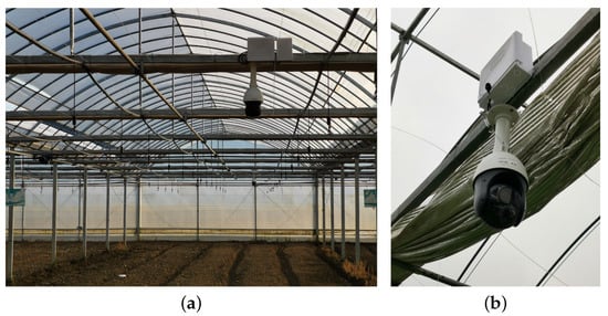
Figure 1.
Installation of camera in greenhouse. Sub-figure (a) shows the installation location in the greenhouse and Sub-figure (b) shows the camera details.
A total of six image sequences of green leafy vegetable growing were collected, two for 17 days, two for 15 days and two for 14 days. The images, each with a resolution of pixels, contain dozens of growing leafy greens. The images were taken by fixed cameras at roughly the same intervals every day. All images were manually annotated to record the shape of each plant in the form of edge points. A schematic diagram of the annotation results is shown in Figure 2b. These 92 images form the testing set of this paper, which contains 4899 leafy greens. In addition, the same green leafy vegetable in different images was labeled as a fixed and unique ID to test the leafy green tracking algorithm. A total of 321 different leafy greens were labeled across images.
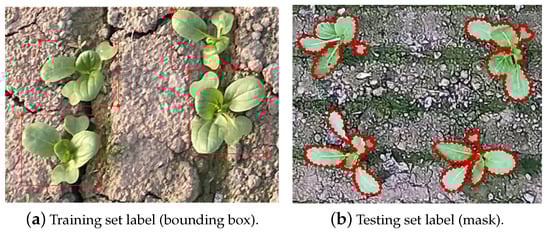
Figure 2.
Annotation results of edge points of green leafy vegetables. The annotations for the training set, shown in Sub-figure (a), are bounding boxes. The annotations for the testing set, shown in Sub-figure (b), are masks.
In order to train the data-driven model for green leaf vegetable segmentation, more images were further collected using fixed cameras and smartphones to construct the training dataset. The leafy greens in these images are only labeled as bounding boxes because the labeling of pixel mask is too laborious. The annotation format is shown in Figure 2a. The effort to label bounding boxes is tens of times less than that for masks. However, due to incomplete labeling information, previous segmentation algorithms [5,9,10] cannot be trained directly. In this paper, weakly supervised learning based on boundary boxes is employed to train the instance segmentation model of leafy green vegetables.
Since the leafy green vegetables at the edges of the images taken by mobile devices are not strictly vertical looking down, we split the images into small patches, keeping only the parts that are similar to images taken by fixed cameras. We obtained 548 images with a resolution of by this method. In addition, 54 images were obtained by the fixed camera, but due to the limitation of the memory size of the GPU (Graphics Processing Unit) used in this paper, these images cannot be directly trained with the resolution of pixels. Therefore, these images were divided into 108 local images of pixels by the similar image block partitioning approach.
Finally, the composition of the training set and testing set is shown in Table 1. Since there is no obvious sequence relationship in the images of the training set, the plant number cannot be marked. In fact, this hybrid training set is very similar to real agricultural production applications.

Table 1.
The composition of training and testing set after preprocessing.
3. Methods
As introduced in Section 1, each leafy green vegetable is segmented to obtain its top-view projection. In order to reduce the interference caused by similar background and illumination variation, this paper achieves segmentation of leafy green vegetables based on a deep convolutional neural network. Different from previous methods [9,10,11], this paper adopts a weakly supervised learning method [12]. In the training stage, only bounding box level annotation is needed to complete model parameter learning. This approach will be described in detail in Section 3.1.
In order to continuously analyze the phenotypic changes of a plant, it is necessary to track each leafy green vegetable after obtaining the top-view projection. This paper conducts the tracking of leafy green vegetables based on position and shape information. The detailed method will be introduced in Section 3.2.
3.1. Weakly Supervised Instance Segmentation of Leafy Greens
In order to obtain phenotypic information such as quantity and top-view area of leafy green vegetables in the planting environment, this paper conducts instance segmentation of leafy green vegetables based on deep convolutional neural network. Related technology has been studied in the field of computer vision and achieved excellent results on various datasets [9,10,11,13,14,15]. However, training such an instance segmentation model requires a large amount of pixel-level mask annotation data. It often takes several hours to label the pixel mask of an image, which seriously affects the application of relevant algorithms in practical applications.
In 2021, Tian et al. [12] proposed BoxInst (High-Performance Instance Segmentation with Box Annotations), which uses only box-level annotation to train the instance segmentation model. By employing the same neural network structure as CondInst (Conditional Convolutions for Instance Segmentation) [15], BoxInst first predicts the object category and a controller corresponding to each Region of Interest (RoI), and then convolves the mask feature of the image with the controller to predict the pixel mask of the object. Different from Condinst, Boxinst replaces Dice Loss with Projection Loss and Pairwise Affinity Mask Loss, so that training could be carried out based on bounding box annotation.
In this paper, the color similarity calculation involved in Pairwise Affinity Mask Loss is transferred to Excess Green (ExG) feature space [16] to improve the accuracy of green leaf segmentation, and an adaptive weed filtering algorithm based on area threshold, K-means clustering and time context constraint is proposed. The work is described in more detail below.
The key to weakly supervised learning of instance segmentation is Projection Loss and Pairwise Affinity Mask Loss. Projection Loss aims to learn the instance location by the bounding box annotation. Formalized, box label is denoted as b, and object mask predicted by neural network is denoted as . and are both projected along the x-axis and y-axis, and the projected vectors are called and , respectively.
where and represent the projection along the x-axis and y-axis, which can be obtained by taking a maximum in the y direction () and a maximum in the x direction () respectively.
The projection loss is defined as
where is Dice Loss.
Pairwise Affinity Mask Loss is employed to learn instance shapes. Consider pixels , , and their mask prediction results , , is defined as the label of edge between them. An edge can be regarded as an association between two pixels. If two pixels belong to the same mask then , otherwise . The probability that is
The probability that is
The Pairwise Affinity Mask Loss is defined as
where is the set of edges whose endpoints are in the plant bounding boxes.
Finally, the two losses are added together to form the loss function of the segmentation model
Under the weakly supervised condition with only bounding box annotation, there is no pixel-level ground truth to calculate Pairwise Affinity Mask Loss. Based on the observation of mask labels, a hypothesis can be made that pixels with similar colors are more likely to be on the same mask [12]. Define the color similarity as
where and are the color vectors of pixels (i, j) and (l, k). is a constant, default as 2. If the color similarity of the two pixels is greater than the threshold , the two pixels are considered to be on the same mask, and the label of the edge between them is 1. Therefore, Pairwise Affinity Mask Loss can also be expressed as
where is the indicator function, is a constant threshold, default as 0.1. Compared to Equation (8), Equation (11) contains only the positive term.
In the original Boxinst, Tian et al. [12] calculated color similarity after converting RGB images into LAB color space, because LAB representation is closer to human visual perception mode. In the segmentation task of leafy green vegetables in the planting environment, ExG (Excess Green) feature can suppress the interference of shadow, dead grass, soil and other environmental noises. Therefore, in this paper, the calculation of color similarity is converted to ExG feature space to make a better distinction between leafy green vegetables and the background. Formally, the calculation method of ExG is
where is the ExG value of pixel , and is the pixel value of green, blue and red channels in RGB representation of pixel
Equation (10) can also be further expressed as
This paper constructs neural network based on ResNet50 (Residual Network) [17] to achieve the balance between fitting ability and data scale. After the backbone network, different depth features are fused through FPN structure [18], and the mask prediction network proposed by CondInst is connected behind each feature layer. Complete model inference and mask loss calculation process are shown in Figure 3. Other parts not mentioned, such as classification and regression loss, are the same as CondInst [15].
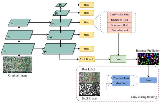
Figure 3.
Schematic diagram of leafy greens segmentation neural network.
In the planting environment, weeds similar to leafy green vegetables can seriously affect phenotype analysis. Due to the similar appearance, the instance segmentation algorithm is prone to false positives, misidentifying weeds as leafy greens. In this case, some additional post-processing is needed to achieve weed filtering.
Fortunately, the top-view projected area of weeds is often significantly smaller than that of leafy green vegetables. Therefore, the area distribution of all instances in the image can be analyzed by top-view projected area histogram. As can be seen from Figure 4, there is a deviation between the area distribution of weeds and leafy green vegetables, so it is feasible to filter weeds through analyzing the top-view projected area.
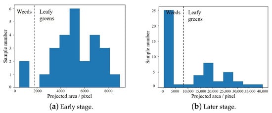
Figure 4.
Histogram of predicted instance pixel area statistics. In the early stage, the number of weeds is small, as shown in Sub-figure (a). In the late stage, the number of weeds may be large, as shown in Sub-figure (b).
A naive idea is to filter weeds by an area threshold. Calculate the mean top-view projected area of all detected instances in the image
where is the mean projected area on n-th day, is the projected area of plant , is all instances detected on n-th day. Then only the instance whose projected area is greater than can be retained. Where is the area threshold, which is used to adjust the degree of weed filtering. However, when the number of weeds is very high, shown as Figure 4b, the mean projected area of all instances will be pulled down, leading to weeds leakage.
Aiming at the situation of too many weeds, this paper proposed to distinguish weeds and leafy green vegetables by K-means clustering algorithm. As can be seen from Figure 4, the projected area of weeds and leafy green vegetables has actually become two clusters at this time. Therefore, the projected area can be processed by K-means algorithm, and all detected instances can be divided into two clusters. Then, according to the mean area of the two clusters, which cluster belongs to leafy green vegetables can be concluded.
By analyzing the top-view projected area histogram, area threshold method or K-means clustering method can be adaptively selected. The top-view projected area of all instances in the image is divided into 10 intervals between the minimum and maximum values for histogram statistics. If sample number in the leftmost interval is less than the threshold , the area threshold method is adopted; otherwise, K-means clustering method is adopted. However, considering that the clustering results may be unreliable, it is necessary to calculate whether the ratio of the mean area of the two clusters meets Equation (15) after clustering.
where and are the clustering center values. If Equation (15) is not satisfied, it means K-means cannot divide the object into two clusters of leafy green vegetables and weeds. In this case, area threshold method is still used to replace K-means for weed filtering. In Section 3.2, the robustness of weed filtering is improved by adding time context constraints, which will be discussed later.
After the leafy greens segmentation and weed filtering, the mean top-view projected area of all non-edge leafy greens in the image can be counted, and its change can be continuously analyzed to judge whether the overall growth is in line with expectations.
3.2. Data Association for Phenotype Tracking
Monitoring and analyzing the phenotypic changes of a vegetable over several days requires multi-object tracking of vegetables in the image. In recent years, most of the work on multi-object tracking focuses on pedestrian and vehicle tracking [19,20,21,22,23]. In these tasks, an object’s position is difficult to predict, but the appearance change is relatively small, so the related work [20,21,23] mainly focuses on building an appearance model to achieve effective multi-object tracking. However, during the growth of leafy greens, the appearance of the same vegetable changes considerably, and the appearance difference between different vegetables is relatively small, which makes the appearance characteristics not robust enough in vegetable tracking. Fortunately, there is little position change during the growth of leafy greens, so it is possible to track leafy greens based on location information [19].
Firstly, the segmentation results of the 1st day are initialized into several tracking tracks of leafy greens, and then the growth tracks of leafy greens are updated iteratively. Suppose instances are segmented and tracked on n-th day and instances are segmented on -th day. The corresponding relationships of these instances and tracks are obtained by Hungarian matching [19].
The i-th instance tracked on the n-th day is denoted as , then the j-th instance detected on the -th day can be denoted as . Calculate the mask intersection over union (mask IoU) of and by
where is the number of pixels at the intersection of two masks, is the number of pixels in the union of the two masks. Here, mask IoU is calculated instead of box IoU like SORT (Simple online and realtime tracking) [19], because mask IoU can also contain shape information in addition to location information. A larger mask IoU can be obtained only when two leafy greens have similar positions and shapes.
Traversing all instances will yield IoU values, which can form a matrix of size
Then, an IoU threshold is used to determine whether and could be considered the same vegetable. Formally, set the elements of matrix that are less than to 0 and obtain matrix
Take negative values of all elements in , which minimizes the cost between the two plants with the largest IoU, and the cost matrix is obtained
According to the cost matrix , the bipartite graph matching problem is solved by Hungarian matching [19], and the maximum matching of the bipartite graph is found as the result of the data association of leafy green vegetables. When there are multiple maximum matches, the match with the minimum sum of edge costs is selected.
During the growth of leafy green vegetables, there are some vegetables that gradually died or sprouted, which makes the number of tracked leafy green vegetables change dynamically. Therefore, after the bipartite graph matching is completed, it is necessary to update the tracks, delete the tracks without corresponding segmentation results for 2 days (may be dead), and initialize the leafy green vegetables without the corresponding track into a new track (may be new germination).
After obtaining the leafy greens’ tracking information, time context constraint can be added to weed filtering to prevent the leafy green vegetables from being filtered by mistake. Before adaptive weed filtering, can be calculated by Equation (18). After that, calculate the maximum value of each row in and define it as
is called the protection vector. If the i-th element of is greater than 0, it indicates that the i-th vegetable has a high probability of being associated with the previous track, so this vegetable should be protected so that it will not be filtered out as a weed. After the calculation of the protection vector, the unprotected mis-segmented projection is removed by the adaptive weed filtering algorithm. Finally, the Hungarian algorithm is used to solve the bipartite graph matching and dynamically update the leafy greens tracks.
When there are many leafy greens in the image, they require a large amount of computation to calculate the Mask IoU matrix, which makes the weed filtering algorithm with time context constraint time-consuming. In fact, the matrix used in weed filtering and plant tracking only needs to be computed once. Firstly, between all segmentation projections and tracking tracks is calculated. After the weed filtering is completed, several rows corresponding to weeds are supposed to be removed, and a new matrix is obtained for the bipartite graph matching during plant tracking. This method can reduce the influence of time context constraint on the overall algorithm speed.
By tracking vegetables through data association, we can analyze the phenotypic change of a vegetable over time. For example, judging whether the growth of a vegetable is in line with expectation through the change of top-view projected area for several days. Normally, the top-view projected area of a leafy green will continue to increase. If the top-view projection area of a vegetable does not grow and the projection area is smaller than others, the growth of the vegetable is stagnant, and problems such as water shortage may occur. Formally,
where is the projected area of the i-th vegetable on n-th day, d is a hyper-parameter, represents the time window length of phenotypic analysis, is the mean projected area of n-th day, is a constant number, default as 0.6.
When the phenotypic changes of leafy green vegetables are only considered for 1 day, the identification of abnormal growth plants is easily disturbed by some environmental changes. Therefore, abnormal plant identification is achieved by considering phenotypic changes for consecutive d days. The corresponding phenotypic analysis results can be obtained by adjusting the value of d according to actual problems. When , the influence of wind, sun and other environmental factors can be excluded, and the abnormal plants can be identified within 2 days.
To prevent interference from plants appearing only partially in the image, the abnormal plant identification is performed only for plants appearing completely in the image (not at the edge of the image). Considering the possible interference caused by occlusion, abnormal growth can be considered only when the sum of Mask IoU of the i-th plant and other plants is small (less than the threshold ).
4. Results
4.1. Implementation Details
The computing platform used in this paper is as follows: the central processing unit (CPU) is Intel(R) Xeon(R) Silver 4110 CPU @ 2.10 GHz × 2, the graphics processing unit (GPU) is Nvidia Geforce RTX 2080Ti × 4, memory is 64 GB, the operating system (OS) is Ubuntu16.04 and the compute unified device architecture (CUDA) version is 10.0.
The deep neural network in this paper is implemented by PyTorch framework, version 1.6.0. The rest of the code is implemented in Python at version 3.8. In the training phase, the following hyper-parameters are chosen: the optimizer is mini-batch SGD; the number of training steps is 5000; the batch size is 4; the learning rate is 0.005 with warm up. .
4.2. Results of Instance Segmentation
The instance segmentation model introduced in Section 3.1 is trained with the configuration in Section 4.1, and the model is evaluated on the testing set. The effectiveness of the proposed method is evaluated by Precision, Recall and F1-score. Weed filtering is not carried out in the calculation of the evaluation indexes, because weed identification is also an ability that instance segmentation models should have. The results of instance segmentation are shown in Table 2, which shows that weakly supervised learning based on color similarity of ExG feature achieves excellent results. While Recall is pretty high, the model trained through ExG similarity predicts less false detection, and its Precision is significantly higher than LAB model. Visualized segmentation results of leafy greens are shown in Figure 5. The shape and location of leafy greens are well predicted, but some weeds are detected incorrectly.
Table 2.
The results of instance segmentation on testing set. The confidence threshold is 0.5. The IoU threshold is 0.5. Bold is the best result compared with other methods. * indicates that the model training time is longer. All model results are without weed filtering.
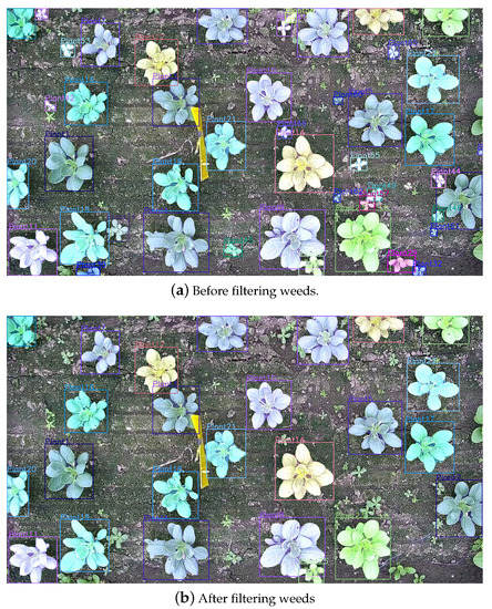
Figure 5.
Comparison of weeds before and after filtering. As shown in Sub-figure (a), some objects are misidentified as leafy greens. After filtering weeds, objects that are mistakenly identified as leafy greens are removed, as shown in Sub-figure (b).
Then, the weed filtering approach proposed in Section 3.1 is carried out for post-processing. The results of weed filtering are also shown in Figure 5. The adaptive weed filtering algorithm proposed in this paper can filter out most of the mistakenly detected weeds, so as to better analyze the phenotype information of leafy green vegetables.
4.3. Results of Instance Tracking
The proposed leafy greens tracking method is tested on the testing image sequences introduced in Section 2, and the results are shown in Table 3 and Figure 6. The indicators in Table 3 are from the work of Voigtlaender et al. [22], which are employed to measure the accuracy of multi-object tracking and segmentation. Leafy greens tracking is performed on the basis of instance segmentation. With 0.5 as the IoU threshold, correct segmentation results are denoted as TP, false detection as FP, and missed detection as FN. In addition, MOTS (multi-object segmentation and tracking) also requires the same tracking ID allocated to an object in adjacent frames, otherwise, it is denoted as IDS (ID switch). Note that FP, FN and IDS are wrong track results. From this, MOTSA can be calculated as
where and represent the number of samples with correct segmentation, false detection, missed detection and ID switching, respectively, and represents the total number of samples segmented. In order to measure the overlap between tracking result and ground truth, MOTSP is defined as
where is the segmented result and is the ground truth. Furthermore, if we replace with , sMOTSA can be obtained through
This index not only reflects the overlap between the segmentation result and the ground truth, but also contains the related index of the data association result, which can reflect the effect of MOTS comprehensively.
Table 3.
The results of leafy greens tracking on testing set. Bold is the best result compared with other methods. * indicates that the model training time is longer, the learning rate is 0.01, and the number of training steps is 8000. sMOTSA can be seen as a combination of MOTSA and MOTSP.
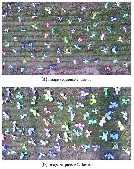
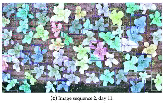
Figure 6.
Visualized results of leafy greens instance tracking. Each leafy green has a unique ID that remains the same during tracking and is noted in the upper left corner of the bounding box. Sub-figure (a–c) are visualized results in 3 different days.
The proposed tracking algorithm of leafy green vegetables based on location information fits the task characteristics well. In the case of weakly supervised training of segmentation model, sMOTSA has reached 76.3. In addition, the tracking algorithm is also tested without weed filtering and without time context constraints, as shown in Table 3. When weed filtering is not carried out, many weeds are mistakenly considered as leafy greens, resulting in a large number of false positives, which leads to the decrease of sMOTSA and MOTSA. When the time context constraint is not used in weed filtering, leafy green vegetables may be mistakenly removed, resulting in false negative and a decrease in the indexes. The green leaf segmentation model trained by LAB color similarity predicts more false positives, and its sMOTSA index is still low even after weed filtering and training more steps. In general, the model trained by ExG similarity with adaptive weed filtering achieves better tracking results of leafy green vegetables.
As can be seen from the results of Figure 6, the tracking ID of leafy green vegetables maintain a good consistency with few mismatches. The bipartite graph matching based on mask IoU measure in this paper can effectively achieve the tracking of leafy greens, so as to continuously monitor their growth status.
In terms of speed, the average inference time for instance segmentation of 92 images with resolution in the test set is 0.88 s. When the time context constraint is not employed, the average time of weed filtering is 0.34 s. When the time context constraint is used, because each sequence contains up to 53 leafy greens on average, the amount of calculation of Mask IoU is large, and the average time of weed filtering is 1.14 s. Furthermore, it takes 0.83 s on average to conduct plant tracking.
According to the calculation method of the shared Mask IoU matrix of weed filtering and plant tracking introduced in Section 3.2, the total average time consumed by plant segmentation, weed filtering and plant tracking is 2.36 s, 0.49 s less than before optimization, and 0.31 s more than without the time context constraint. This meets the application requirements in agricultural scenarios.
4.4. Results of Growth Monitoring
After the instance segmentation of leafy green vegetables, the mean top-view projected area of leafy greens in which the top-view projection completely appeared in the image is calculated and plotted as a curve by day. However, it can be seen from Figure 5 and Figure 6 that there are small gaps between the leaves of leafy green vegetables, which can hardly be predicted in the top-view projection generated by instance segmentation. The projected area predicted by the model in this paper is slightly larger than the real projection. Considering that this phenomenon is widespread, the mean top-view projected area can be multiplied by a constant of 0.95 as a gap penalty to further improve the accuracy of phenotypic calculation. The mean top-view projected area prediction errors of each growth sequence in the testing dataset are shown in Table 4.
Table 4.
Mean area error and error with gap penalty of testing set. Bold is the best result compared with other methods. * indicates that the model training time is longer.
As can be seen from Table 4, the accuracy of phenotypic analysis can be further improved by adding gap penalty to the predicted results. However, this penalty is not effective for the models trained by LAB color representation, because although these models also have the problem of too large segmentation results, they mistakenly identify too many weeds with small area as leafy green vegetables, resulting in the predicted mean area being lower than the true value. On the whole, the model trained by ExG similarity has the best effect.
Taking an image sequence as an example, the curve of its mean top-view projected area changing with days is drawn in Figure 7. The predicted curve can reflect the trend of the top-view projection of leafy green vegetables as well as the real curve. On the 12th and 16th days, the intense light and lack of water caused the contraction of the leaves of most leafy green vegetables, and the model trained in this paper could capture this phenomenon and provide timely warning. The image of leafy green vegetables on the 12th day is shown in Figure 8.
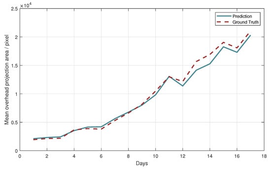
Figure 7.
The mean top-view projected area of image sequence 1 varies with date. The solid line is the prediction result of the model, and the dotted line is the annotation result. Only the vegetables in which the top-view projection all appeared in the image were included in the statistics.
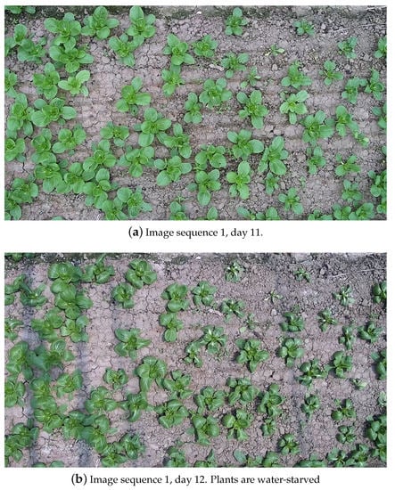
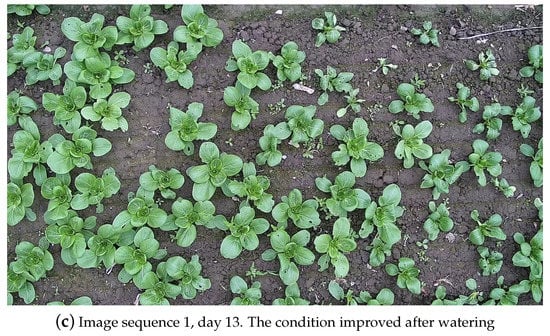
Figure 8.
Images from day 11 to day 13 day in image sequence 1. As a result of the day light intensity caused water shortage, leafy green vegetables appear leaf shrinkage phenomenon, as shown in the change between Sub-figure (a,b). After watering, most of the plants returned to growth, as shown in Sub-figure (c).
After the leafy green tracking is completed, changes in the top-view projected area can be continuously monitored during the growth of a vegetable, so as to analyze the current growth status. Figure 9 shows the curves of the top-view projected area during the growth of two leafy vegetables.
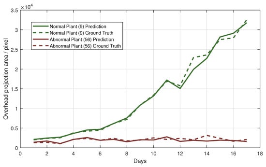
Figure 9.
Top-view projected area curves of two leafy greens during their growth.
According to Equations (21) and (22), abnormal growth vegetables in the image are identified, and the visualization results are shown in Figure 10. This section identifies abnormal growth plants based on 2-day phenotypic changes, which means in the Equation (21). In the 321 tracking sequences of leafy green vegetables in the test set, 11 tracking sequences are abnormal, showing the trend of wilting and death, and the other 310 sequences show normal growth status. According to Equations (21) and (22), 10 abnormal growth sequences are correctly identified, 1 abnormal growth sequence is misclassified as normal, 5 normal sequences are misclassified as abnormal, and the remaining 305 normal sequences are correctly classified. As can be seen from the visualization results in Figure 10 and the quantitative experiment results, after the segmentation and tracking of leafy green vegetables, abnormal growth plants can be found and alerted by monitoring the top-view projected area, which has application potential in fine cultivation of plants.
Figure 10.
Visual results of abnormal plant detection considering the 2-day phenotypic changes. Cyan means normal leafy greens and red means abnormal leafy greens.
5. Discussion
The phenotype analysis of leafy green vegetables in the planting environment is easily affected by light changes and interference of similar objects, resulting in inaccurate perception results. Phenotype analysis based on deep convolutional neural network has good robustness, but requires a large amount of annotated data to train the model. In this paper, the latest weakly supervised deep convolutional neural network training method [12] is introduced into the field of phenotype analysis and optimized for the specific task of leafy green vegetable phenotype analysis. The results in Table 3 show that compared with the original method [12], the calculation of Pairwise Affinity Mask Loss based on ExG color similarity can improve the accuracy of green leafy vegetable instance tracking because of a lower false positive (FP) rate. In ExG space, as in shadows, dead grass and other disturbances are suppressed, the distinction between leafy green vegetables and environmental background is clearer. Algorithms fine-tuned with domain knowledge are better suited to specific tasks.
In real environments, weeds interfere with phenotype perception of leafy greens. However, after tilling and weeding prior to sowing, the later-spreading weeds will germinate later than the planted crops, allowing the projected area to filter out misidentified weeds. In this paper, adaptive weed filtering based on area threshold method and K-means clustering method is proposed, and leafy green vegetables are protected from misscreening according to the time context information of phenotype tracking. After the weeds are filtered, the number of leafy green vegetables in the image and the mean top-view projected area can be calculated, so as to analyze whether there is stress such as excessive light at present, and a timely alarm can ensure that intervention measures can be taken quickly. Figure 5, Figure 7 and Figure 8 show the effectiveness of this approach. Compared with explicitly labeling weeds and training the segmentation model of leafy greens and weeds, the proposed algorithm requires less manual labeling and is more suitable for the application with limited labels.
Currently, few phenotype analysis studies can track plant phenotype changes in cropping environments without affecting plant growth. Most of the work that exists is done in simple laboratory environments [5] or does not utilize time-context information [6]. This paper presents a basic scheme based on bipartite graph matching with mask IoU measure to conduct leafy greens tracking. We found that the tracking of leafy greens is accurate enough by position modeling, as shown in Figure 6.
Finally, on the basis of phenotypic tracking, we tried the growth abnormality detection task, which could detect the abnormal greenhouse environment, as shown in Figure 7, and abnormal leafy green plants, as shown in Figure 9 and Figure 10. Different from previous work, this paper analyzed the leafy greens separately on the basis of tracking, and the results were more conducive to fine cultivation. In the framework of phenotypic tracking, maturation prediction and other tasks can be further studied in the future.
The method in this paper also has some limitations, such as the fact that it is only applicable to the early and middle period of crop growth. When the crops are approaching maturity, the overhead projection area can no longer reflect their growth conditions due to the large overlap between them. At these times, however, crops are more resistant to environmental disturbances and the need for real-time monitoring is not as great as it once was.
6. Conclusions
In this paper, a weakly supervised instance segmentation algorithm with deep convolutional neural network is introduced into phenotype analysis. Then, a weed filtering algorithm based on area threshold, K-means clustering and time context constraint is proposed to deal with the disturbance of weeds in planting environment. Thirdly, the bipartite graph matching based on mask IoU measure is employed to track leafy green vegetables. In the framework of phenotype tracking, global and single plant growth monitoring and abnormal condition detection are implemented. Experiments show that the proposed method can achieve 0.95 F1-score and 76.3 sMOTSA. Compared with the fully supervised approach, the workload of agricultural data annotation required by the proposed method is significantly reduced, which has potential in practical applications.
In the future, the detailed effect of leafy green vegetable instance segmentation can be further optimized. In addition, more tasks such as maturation prediction can be implemented under the phenotype tracking framework.
Author Contributions
Conceptualization, F.S.; data curation, Z.Q. and J.S.; funding acquisition, F.S.; methodology, Z.Q.; project administration, F.S.; software, Z.Q.; supervision, F.S.; visualization, Z.Q.; writing—original draft, Z.Q.; writing—review and editing, J.S. and F.S. All authors have read and agreed to the published version of the manuscript.
Funding
The research presented in this paper was supported in part by Shanghai Agriculture Applied Technology Development Program, China (Grant No. 2020-02-08-00-07-F01480).
Data Availability Statement
The data presented in this study are available on request from the corresponding author.
Conflicts of Interest
The authors declare no conflict of interest.
References
- Ubbens, J.R.; Stavness, I. Deep Plant Phenomics: A Deep Learning Platform for Complex Plant Phenotyping Tasks. Front. Plant Sci. 2017, 8, 1190. [Google Scholar] [CrossRef] [PubMed]
- Aich, S.; Stavness, I. Leaf Counting with Deep Convolutional and Deconvolutional Networks. In Proceedings of the 2017 IEEE International Conference on Computer Vision Workshops (ICCVW), Venice, Italy, 22–29 October 2017; pp. 2080–2089. [Google Scholar] [CrossRef]
- Dobrescu, A.; Giuffrida, M.V.; Tsaftaris, S.A. Leveraging Multiple Datasets for Deep Leaf Counting. In Proceedings of the 2017 IEEE International Conference on Computer Vision Workshops (ICCVW), Venice, Italy, 22–29 October 2017; pp. 2072–2079. [Google Scholar] [CrossRef][Green Version]
- Chen, Y.; Ribera, J.; Boomsma, C.; Delp, E.J. Plant leaf segmentation for estimating phenotypic traits. In Proceedings of the 2017 IEEE International Conference on Image Processing (ICIP), Beijing, China, 17–20 September 2017; pp. 3884–3888. [Google Scholar] [CrossRef]
- Payer, C.; Štern, D.; Neff, T.; Bischof, H.; Urschler, M. Instance Segmentation and Tracking with Cosine Embeddings and Recurrent Hourglass Networks. In Medical Image Computing and Computer Assisted Intervention—MICCAI 2018; Frangi, A.F., Schnabel, J.A., Davatzikos, C., Alberola-López, C., Fichtinger, G., Eds.; Springer International Publishing: Cham, Swizterland, 2018; pp. 3–11. [Google Scholar]
- Zhang, L.; Zhang, H.; Chen, Y.; Dai, S.; Li, M. Real-time monitoring of optimum timing for harvesting fresh tea leaves based on machine vision. Int. J. Agric. Biol. Eng. 2019, 12, 6–9. [Google Scholar] [CrossRef]
- Hao, X.; Jia, J.; Mateen Khattak, A.; Zhang, L.; Guo, X.; Gao, W.; Wang, M. Growing period classification of Gynura bicolor DC using GL-CNN. Comput. Electron. Agric. 2020, 174, 105497. [Google Scholar] [CrossRef]
- Ghosal, S.; Zheng, B.; Chapman, S.C.; Potgieter, A.B.; Jordan, D.R.; Wang, X.; Singh, A.K.; Singh, A.; Hirafuji, M.; Ninomiya, S.; et al. A weakly supervised deep learning framework for sorghum head detection and counting. Plant Phenom. 2019, 2019, 1525874. [Google Scholar] [CrossRef] [PubMed]
- He, K.; Gkioxari, G.; Dollár, P.; Girshick, R. Mask R-CNN. In Proceedings of the 2017 IEEE International Conference on Computer Vision (ICCV), Venice, Italy, 22–29 October 2017; pp. 2980–2988. [Google Scholar] [CrossRef]
- Bolya, D.; Zhou, C.; Xiao, F.; Lee, Y.J. YOLACT: Real-Time Instance Segmentation. In Proceedings of the 2019 IEEE/CVF International Conference on Computer Vision (ICCV), Seoul, Korea, 27 October–2 November 2019; pp. 9156–9165. [Google Scholar] [CrossRef]
- Huang, Z.; Huang, L.; Gong, Y.; Huang, C.; Wang, X. Mask Scoring R-CNN. In Proceedings of the 2019 IEEE/CVF Conference on Computer Vision and Pattern Recognition (CVPR), Long Beach, CA, USA, 15–20 June 2019; pp. 6402–6411. [Google Scholar] [CrossRef]
- Tian, Z.; Shen, C.; Wang, X.; Chen, H. BoxInst: High-Performance Instance Segmentation with Box Annotations. In Proceedings of the 2021 IEEE/CVF Conference on Computer Vision and Pattern Recognition (CVPR), Nashville, TN, USA, 20–25 June 2021; pp. 5439–5448. [Google Scholar] [CrossRef]
- Lin, T.Y.; Maire, M.; Belongie, S.; Hays, J.; Perona, P.; Ramanan, D.; Dollár, P.; Zitnick, C.L. Microsoft COCO: Common Objects in Context. In Computer Vision—ECCV 2014; Fleet, D., Pajdla, T., Schiele, B., Tuytelaars, T., Eds.; Springer International Publishing: Cham, Swizterland, 2014; pp. 740–755. [Google Scholar]
- Chen, K.; Pang, J.; Wang, J.; Xiong, Y.; Li, X.; Sun, S.; Feng, W.; Liu, Z.; Shi, J.; Ouyang, W.; et al. Hybrid Task Cascade for Instance Segmentation. In Proceedings of the 2019 IEEE/CVF Conference on Computer Vision and Pattern Recognition (CVPR), Long Beach, CA, USA, 15–20 June 2019; pp. 4969–4978. [Google Scholar] [CrossRef]
- Tian, Z.; Shen, C.; Chen, H. Conditional Convolutions for Instance Segmentation. In Computer Vision—ECCV 2020; Vedaldi, A., Bischof, H., Brox, T., Frahm, J.M., Eds.; Springer International Publishing: Cham, Switzerland, 2020; pp. 282–298. [Google Scholar]
- Woebbecke, D.M.; Meyer, G.E.; Bargen, K.V.; Mortensen, D.A. Color Indices for Weed Identification Under Various Soil, Residue, and Lighting Conditions. Trans. ASAE 1995, 38, 259–269. [Google Scholar] [CrossRef]
- He, K.; Zhang, X.; Ren, S.; Sun, J. Deep Residual Learning for Image Recognition. In Proceedings of the 2016 IEEE Conference on Computer Vision and Pattern Recognition (CVPR), Las Vegas, NV, USA, 27–30 June 2016; pp. 770–778. [Google Scholar] [CrossRef]
- Lin, T.Y.; Dollár, P.; Girshick, R.; He, K.; Hariharan, B.; Belongie, S. Feature Pyramid Networks for Object Detection. In Proceedings of the 2017 IEEE Conference on Computer Vision and Pattern Recognition (CVPR), Honolulu, HI, USA, 21–26 July 2017; pp. 936–944. [Google Scholar] [CrossRef]
- Bewley, A.; Ge, Z.; Ott, L.; Ramos, F.; Upcroft, B. Simple online and realtime tracking. In Proceedings of the 2016 IEEE International Conference on Image Processing (ICIP), Phoenix, AZ, USA, 25–28 September 2016; pp. 3464–3468. [Google Scholar] [CrossRef]
- Wojke, N.; Bewley, A.; Paulus, D. Simple online and realtime tracking with a deep association metric. In Proceedings of the 2017 IEEE International Conference on Image Processing (ICIP), Beijing, China, 17–20 September 2017; pp. 3645–3649. [Google Scholar] [CrossRef]
- Bergmann, P.; Meinhardt, T.; Leal-Taixé, L. Tracking Without Bells and Whistles. In Proceedings of the 2019 IEEE/CVF International Conference on Computer Vision (ICCV), Seoul, Korea, 27 October–2 November 2019; pp. 941–951. [Google Scholar] [CrossRef]
- Voigtlaender, P.; Krause, M.; Osep, A.; Luiten, J.; Sekar, B.B.G.; Geiger, A.; Leibe, B. MOTS: Multi-Object Tracking and Segmentation. In Proceedings of the 2019 IEEE/CVF Conference on Computer Vision and Pattern Recognition (CVPR), Long Beach, CA, USA, 15–20 June 2019; pp. 7934–7943. [Google Scholar] [CrossRef]
- Xu, Z.; Zhang, W.; Tan, X.; Yang, W.; Huang, H.; Wen, S.; Ding, E.; Huang, L. Segment as Points for Efficient Online Multi-Object Tracking and Segmentation. In Computer Vision—ECCV 2020; Vedaldi, A., Bischof, H., Brox, T., Frahm, J.M., Eds.; Springer International Publishing: Cham, Switzerland, 2020; pp. 264–281. [Google Scholar]
Publisher’s Note: MDPI stays neutral with regard to jurisdictional claims in published maps and institutional affiliations. |
© 2022 by the authors. Licensee MDPI, Basel, Switzerland. This article is an open access article distributed under the terms and conditions of the Creative Commons Attribution (CC BY) license (https://creativecommons.org/licenses/by/4.0/).