A Prediction Method of Seedling Transplanting Time with DCNN-LSTM Based on the Attention Mechanism

Abstract

To improve the production efficiency and reduce the labor cost of seedling operations, cabbage was selected as the research subject, and a novel approach based on the attention mechanism combining the deep convolutional neural network (DCNN) and long short-term memory (LSTM) is proposed. First, the cabbage growth data and environmental monitoring data were normalized, and input samples were obtained by sliding the time window. Then, the DCNN and the LSTM were used to extract the spatial feature information and temporal correlation of the samples, respectively. At the same time, the attention mechanism was used to set the weight coefficients of different feature information and highlight the role of the main features of the sample in the model, thereby improving the prediction accuracy. By analyzing the experimental data collected by the Shandong Seedling Plant, the DCNN-LSTM method based on the proposed attention mechanism achieved good prediction results, providing experience for the engineering application of decision-making regarding seedling transplanting time. The experimental data showed that the mean absolute error, root-mean-square error, mean absolute percentage error, and symmetric mean absolute percentage error of the prediction results of this method were 0.356, 0.507, 0.157, and 0.082, respectively. Compared with the CNN, LSTM, LSTM-Attention and CNN-LSTM models, this model showed higher prediction accuracy.

1. Introduction

Cabbage is one of the most consumed vegetables in China and belongs to the Brassica family of cruciferous vegetables [1]. In cabbage production, seedling raising is the primary basis for improving production efficiency. Seedling growth is a dynamic and complex physiological, biochemical, and metabolic process, whose development will directly affect the yield, quality, and safety of the crops. Most of the current crop growth predictions are based on image methods. However, in the case of strong wind, fog, and occlusion, the camera required for these techniques may not be able to obtain clear image data, resulting in reduced prediction accuracy and even misjudgments. Therefore, a prediction method based on seedling growth state and environmental text information with higher applicability to complex environments is urgently needed.

With the high development of artificial intelligence and agricultural Internet of Things technology, the environmental monitoring and regulation technology of facility agriculture are significantly developing. Exploring a method to predict the growth of crops on the basis of environmental factors has become a new research focus and challenge in the 21st century [2,3]. The crop growth monitoring technology can monitor and obtain parameters regarding crop stalk, leaf expansion, leaf size, and plant height in real time. In this way, the data can be used to quantify small changes in crop growth in a short period of time and provide technical support for a timely and accurate vegetable planting management. Research on the influence of various environmental parameters in a solar greenhouse on the growth of cabbage will provide the main theoretical basis for realizing an effective regulation of environmental parameters such as air temperature and humidity, light, soil temperature and humidity, and inferring the growing trend of crops [4,5].

Crop growth prediction is a key part of agricultural precision management [6]. A high-precision growth prediction model based on neural networks and the corresponding crop growth conditions are established according to environmental parameter values that are introduced, which is of great significance for guiding farming. Drees et al. [7] proposed that through the high-throughput imaging sensor measurement and automatic analysis method, the generated images can be automatically interpreted through instance segmentation based on a neural network, and various phenotypic characteristics describing plant growth can be deduced, which provides solutions for plant growth prediction. However, the effect of environmental changes on the growth of seedlings was not considered. Pohan et al. [8] considered the growth environment of seedlings and monitored the growth of seedlings according to temperature, soil moisture, environmental humidity, light intensity, and camera data collected by the Internet network system. A neural network back-propagation method was proposed to evaluate the growth of greenhouse plant seedlings, and a plant seed growth prediction system was developed using computer programming technology. The system generates information based on graphical user interface (GUI) to help check the growth prediction results of greenhouse seedlings, with a data accuracy rate of 92.79%. However, the single evaluation index of this method is only the mean square error, which cannot well reflect the prediction effect of the model. Pezhman et al. [9] proposed a comprehensive model using extreme learning machine (ELM) to predict the final growth of sugarcane and used three evaluation indicators: coefficient of determination, Nash–Sutcliffe efficiency, and root-mean-square error to evaluate the model. Compared with artificial neural network (ANN) and genetic programming models, it provides a faster learning curve and has better generalization ability, but there are fewer comparison models, which represents a disadvantage of the model. Hamid et al. [10] proposed a Beta growth model to predict the emergence time of beet seedlings and the appropriate planting date for beet seeds to overcome weeds under different soil moisture contents, but there is a lack of model comparison analysis. Zhou [11] proposed an improved Elman neural network prediction model to predict the growth situation of rice in different periods in segments, to predict the total yield. However, only the growth of rice in a specific environment was considered, and further verification is needed for variable environments. To solve the prediction problem in a multivariate environment, Meng [12] proposed to build a vegetable growth cycle prediction model under the agricultural cloud platform to provide a guarantee for the integration of vegetable production, supply, and marketing. The cumulative thermoluminescence method accumulation of effective temperature and illumination (AE-TLU) is effective for vegetable growth based on ambient temperature and light intensity, however this method has limitations and is not suitable for root vegetables. For tomato growth prediction, Zhang et al. [13] proposed using agricultural Internet of Things (IoT) sensors to monitor the environmental parameters in the greenhouse and the growth parameters of the tomato body in real time and built a model through the Matlab 2014a platform to study the influence of the greenhouse environmental parameters on the growth of the tomato body. The available information is not considered comprehensive and cannot completely measure the growth of crops. Yang et al. [14] established a tomato growth model that can reflect the dynamic feedback results of the parameters from fruit setting to development and achieved quantitative results on tomato growth, but lacked accurate results. For the prediction of cabbage growth, Yura et al. [15] proposed an image classification method for cabbage seedlings based on convolutional neural networks. By training the model to predict the probability of successful seedling growth, on the test set, AlexNet could accurately classify 94% of the seedlings, but it ignores seedlings with time, as the growth conditions changed. To reduce the limitations of farmers due to lack of scientific knowledge, Susilo et al. [16] established prediction models based on the automatic control retrieval of real-time data, MySQL database storage data, machine learning, and other technologies, but lacked a visual analysis of the model results. Alhnaity et al. [17] proposed a new method for predicting stem diameter growth of agricultural plants, developed an encoder–decoder framework to extract crop features by using long short-term memory (LSTM), and combined the attention mechanism to achieve stem diameter change prediction. Based on the above analysis, researchers established a high-precision growth prediction model through neural networks, which can predict the emergence time, the growth stage of different crops, and the yield, which is of great significance for guiding farming.

To solve the problem of predicting the transplanting time of suitable machine seedlings, a combination of deep convolutional neural network and long short-term memory (DCNN-LSTM) based on the attention mechanism of the transplanting time prediction model is proposed. First, sensor monitoring data and seedling growth measurement data were processed through min–max normalization and sliding time window to eliminate the influence of different dimensions of the sample data. Then, DCNN was used to perform feature learning on the preprocessed data to enhance the model’s ability to extract sample features, and an attention mechanism was introduced into the LSTM to enhance the extraction of the main features of the sample and the learning ability of the model’s time series to achieve transplanting time prediction. Finally, the effectiveness of the proposed method was demonstrated using a dataset established in Shandong Nursery Factory.

2. Materials and Methods

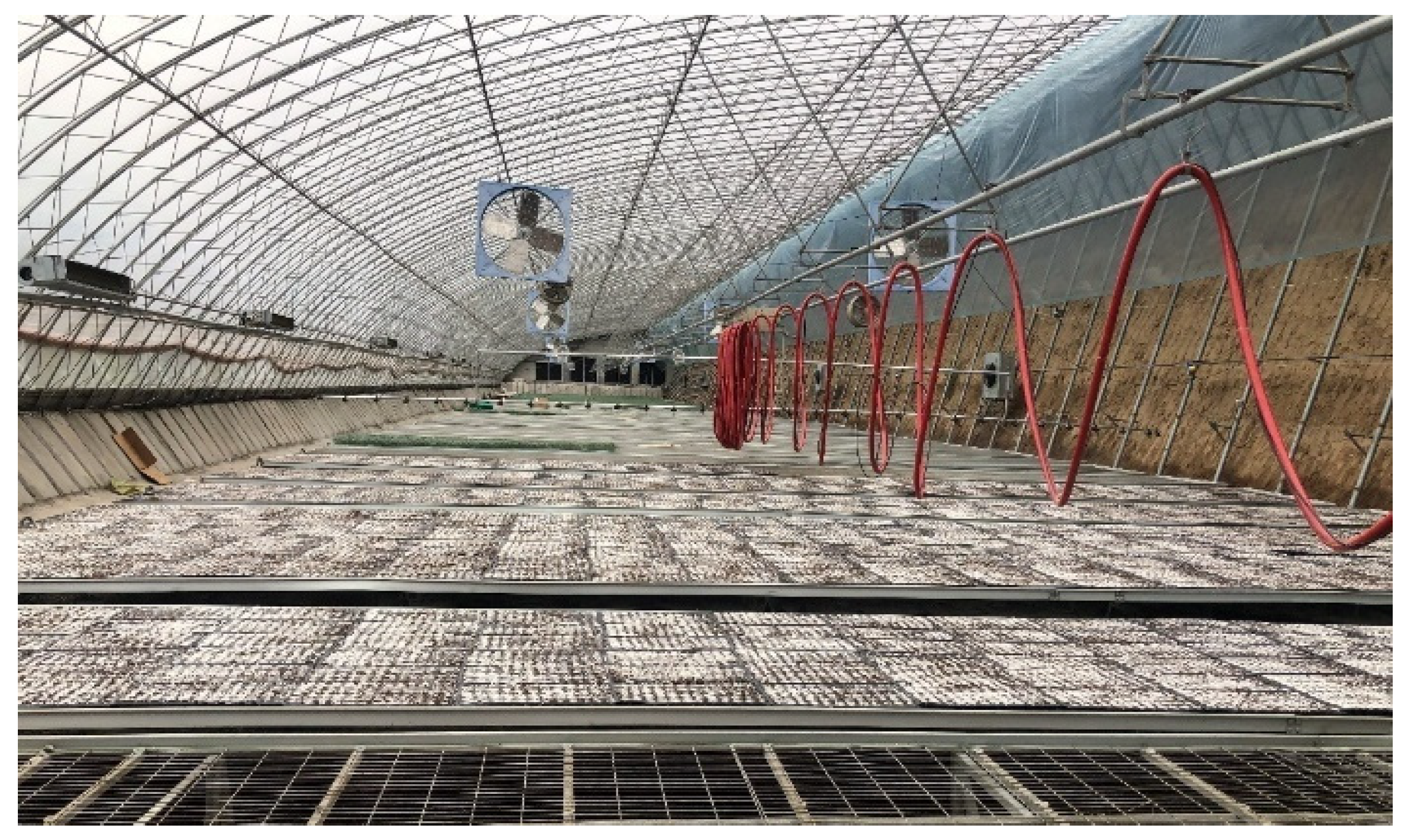
2.1. General Situation of the Test Area

The test was carried out in a large solar greenhouse of Shandong Zibo Seedling Plant from July to August 2021, as shown in Figure 1. The test area is located at 118°44′ E, 36°87′ N. It belongs to the north temperate continental climate, and the average temperature in summer is 18–30 °C. The experimental greenhouse faces east and west, and the crops are cabbage, varieties Zhonggan 21 and purple cabbage. The test time was from sowing of the cabbage to transplanting, and greenhouse management operations, such as irrigation, fertilization, and spraying, were in accordance with the conventional management methods of the seedling plant.

2.2. Experiment Design

In total, 25 samples of Zhonggan 21 and 25 purple cabbage samples were marked at different positions in the seedbed. When the cabbage seedlings emerged, the parameters of the 50 marked samples were measured daily, including plant height, leaf expansion, stem diameter, number of leaves, leaf size, to reflect the growth of the cabbage.

Three air all-in-one sensors were placed on the nursery plant’s wall, at the steel frame’s vent, and near the door. The sensors were developed by Shandong Qiji IOT Technology Co., Ltd. (Zibo, China), and the models were YB5A052300F53F0857, YB5A052300A86A0936, and YB5A052300FF7608EE. We obtained environmental parameters at different locations in the greenhouse: air temperature, relative air humidity, and light intensity. In this experiment, the average value of the three sensors was taken to represent the growth environment of the seedlings. Taking Zhonggan 21 and purple cabbage seedlings marked in solar greenhouse as test samples, the plant growth data and environmental monitoring data were analyzed and modeled, and the effects of the environmental parameters on the growth of two kinds of cabbage seedlings were studied.

3. Data Collection and Processing

3.1. Data Collection

The test data were obtained from the monitoring results of 30 days, from 28 July 2021 to 26 August 2021, and included sensor monitoring values and cabbage growth measurements. Every 24 h, 25 Zhonggan 21 and 25 purple cabbage samples were measured using a vernier caliper. The data included plant height (mm), leaf expansion (mm), stem diameter (mm), number of leaves (pieces), and the length and width of the first four leaves (mm), for a total of 1352 × 12 data, of which, 1352 represents the measured sample size, and 12 represents the eigenvalue. In addition, air temperature (°C), air relative humidity (RH), and light intensity (lx) were obtained through the air all-in-one sensor, with a sampling period of 1 h, with a total of 720 × 3 data, of which, 720 represents the sample size of the sensor, and 3 represents the number of features. The data set used to build the model included values for two varieties, Zhonggan 21 and purple cabbage. Of these, Zhonggan 21 was used as a training set with a total of 676 samples, and purple cabbage was used as a test set with a total of 676 samples; we considered 25 plants for each variety, and the number of features was 16, as shown in

Table 1. Nursery dataset containing 15 characteristic values: seedling height (mm), leaf expansion (mm), stem thickness (mm), number of leaves (pieces), length of the first leaf (mm), width of the first leaf (mm), length of the second leaf (mm), the width of the second leaf (mm), length of the third leaf (mm), width of the third leaf (mm), length of the fourth leaf (mm), width of the fourth leaf (mm), air temperature (°C), air relative humidity (RH), and light intensity (lx).

Subdataset	Variety	Number of Seeding Samples	Number of Features	Sample Size
Training set	Zhonggan No. 21	25	15	676
Test set	purple cabbage	25	15	676

.

3.2. Data Preprocessing

To solve the problem of different dimensions of cabbage growth and environmental monitoring parameters, the normalization method was used to eliminate the unit differences of different parameters, thereby improving the accuracy of the data analysis results.

We defined cabbage sample growth data and sensor monitoring data representation as a sample set $X=\left[x_{i,1},x_{i,2},\dots ,x_{i,j},\dots ,x_{i,n}\right]\in R^{n\times 1}$; ${}^n$ represents the number of features, ${}_i$ represents the number of days, and ${}_j$ represents the sample features. Each parameter value $x_{i,j}$ was normalized [18] and can be expressed as:

$$x=\frac{2(x_{i,j}-x^j{}_{\min })}{(x^j{}_{\max }-x^j{}_{\min })}-1$$

(1)

In the formula, $x$ represents the normalized data, $x^j{}_{\min }$ and $x^j{}_{\max }$ represent the minimum and maximum values of the $j$th feature data, respectively. We avoided a too large input time step of the prediction model, which would lead to the decline of the model prediction performance and training efficiency. This section used the sliding time window method to construct continuous time series features as the input of the model. The set window of length $W_t$ slides along the time axis. At each time step, the input sample size of the prediction model is $W_t\times n$, and the feature data in the window can be obtained. When the computing resources allow it, set the step size of the sliding window to 1 to obtain more data.

4. Predictive Model Building

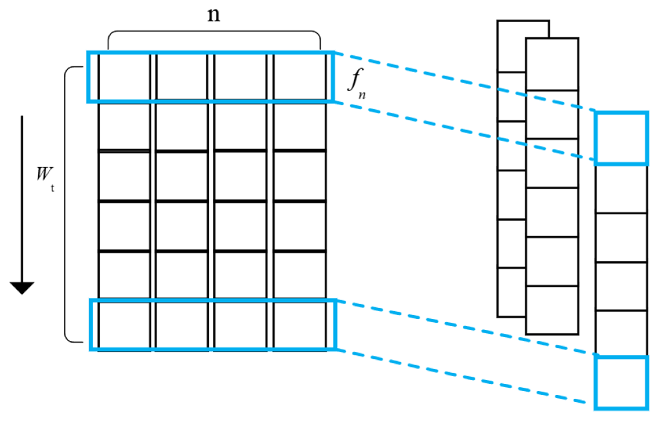
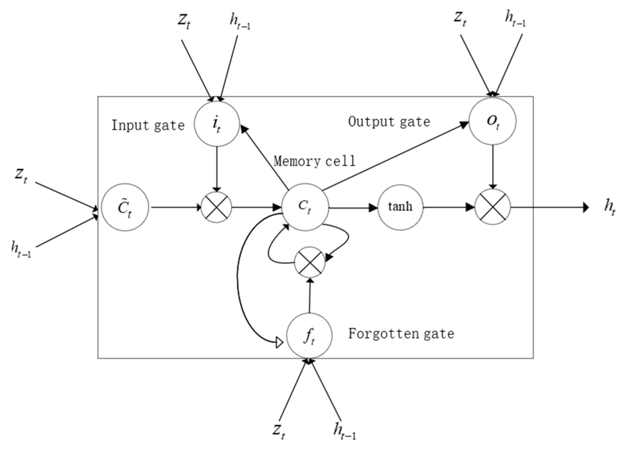
4.1. DCNN-LSTM

The convolutional neural network (CNN) can extract the spatial feature relationship between data after convolution on the input data and has strong feature extraction ability [19,20]. Since the input data are a two-dimensional vector of the number of features and time series, and the one-dimensional convolution kernel can effectively process two-dimensional data, this model adopts a one-dimensional CNN network, and its structure is shown in Figure 2.

After setting the size of the convolution kernel $f_n$, the convolution operation on the input data is as follows:

$$x=\sigma (W_k^T{x}_{i:i}{{}_{+}}_{w_t}{}_{-1}+b_k),0<k\le f_n,k\in Z$$

(2)

In the formula, $\sigma$ represents the activation function of the neuron, $x_{i:i}{}_{+w_t-1}$ represents the input data of the convolution layer, $x$ represents the output data of the convolution layer, $W_t$ represents the size of the time window, $W_k$ and $b_k$ represent the weight and bias term of the $k$th convolution kernel, respectively.

As a variant of the recurrent neural network, LSTM selectively memorizes long-term and short-term information by introducing a “gate” structure and realizes the logical association between long-term and short-term information [21]. The LSTM unit structure is shown in Figure 3 and consists of an input layer, a hidden layer, and an output layer. The basic unit of the hidden layer has data storage capacity, including a gating unit and a memory unit, which can control the flow of information.

The gating unit consists of an input gate, an output gate, and a forget gate, which can selectively decide whether information can pass through. The input gate $i_t$ selects new information to record in the unit, the forget gate $f_t$ selectively forgets the information in the state of the unit, and the information continues to pass through the output gate. The calculation formulas of input gate $i_t$, forget gate $f_t$, and output gate $o_t$ are as follows:

$$i_t=\sigma (W_i{x}_t+W_i{h}_{t-1}^{}+b_i)$$

(3)

$$f_t=\sigma (W_f{x}_t+W_f{h}_{t-1}+b_f)$$

(4)

$$o_t=\sigma (W_o{x}_t+W_o{h}_{t-1}+b_o)$$

(5)

The memory unit $C_t$ can store important long-term memory information, and the calculation formula is:

$$\widetilde{C_t}=\tanh (W_c{x}_t+W_c{h}_{t-1}+b_c)$$

(6)

$$C_t=f_t{C}_{t-1}+i_t\widetilde{C_t}$$

(7)

$$h_t^{}=o_t\cdot \tanh (c_t)$$

(8)

In the formula, $\widetilde{C_t}$ represents the temporary memory unit, $h_t$ represents the state output unit, $\sigma$ represents the sigmoid activation function, $W$ represents the weight, and $b$ represents the bias term.

Aiming at the problem of poor generalization ability caused by model overfitting, L2 regularization to each convolutional layer is added and the LSTM layer can limit the neural network to learn high-frequency components and tend to low-frequency smooth functions, thereby alleviating overfitting. The calculation is as follows:

$$C=C_0+\frac{\lambda }{2n}{\displaystyle \sum _w{w}^2}$$

(9)

where $C_0$ represents the RMSE loss function, $\lambda$ is the regular term coefficient, $w$ is the weight, and $n$ is the number of weight parameters.

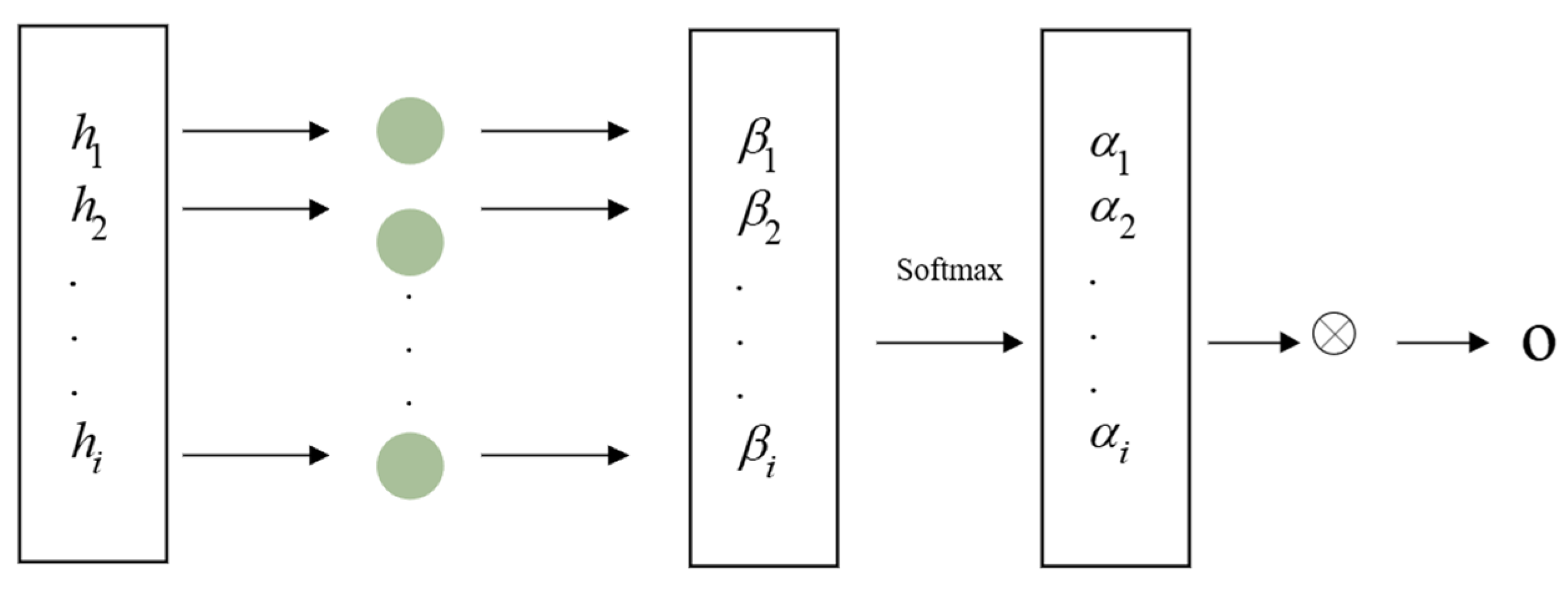
4.2. Attention Mechanism

The attention mechanism is based on the human cognitive ability to process more important information with limited energy [22]. To improve the prediction ability of the model, this paper intriduced the attention mechanism to further assign different weight coefficients to the features extracted by the LSTM. The Attention structure is shown in Figure 4. The Self-Attention module applies t shared weights and biases to the t time-related feature vectors learned by the LSTM. After obtaining the weights of each feature, the weighted summation method was used to finally achieve deep-level feature mining. The calculation formula is as follows:

$${\beta }_i=\sigma (W_i{h}_t+b_i)$$

(10)

$$a_i=softmax({\beta }_i)=\frac{\exp ({\beta }_i)}{{\displaystyle {\sum }_i\exp ({\beta }_i)}}$$

(11)

$$O=H\otimes a_i$$

(12)

In the formula, $W_i$, $b_i$ represent the weight matrix and bias vector between neuron nodes $\sigma$, respectively, ${\beta }_i$ represents the activation function, $a_i$ represents the importance of the feature, $O$ represents the attention weight and represent the output prediction result.

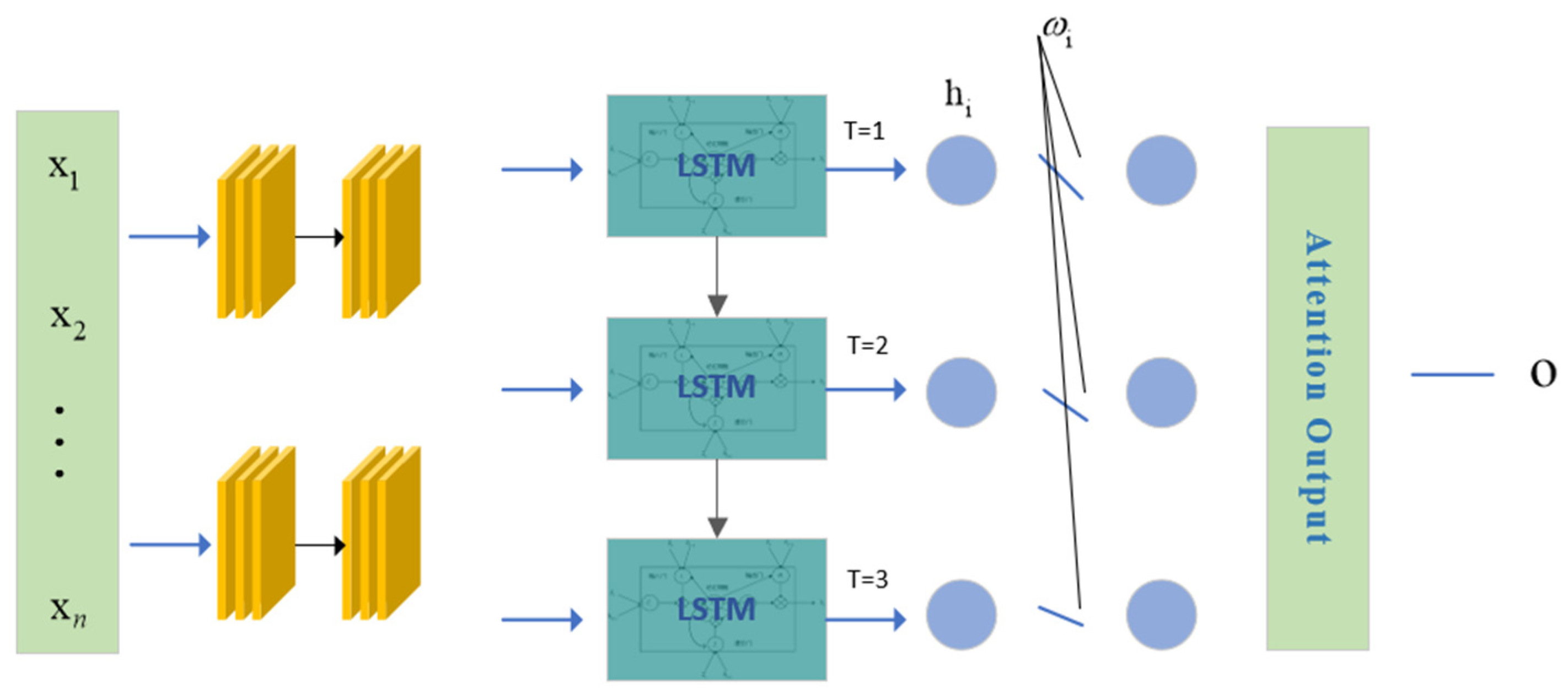
4.3. Attention-Based DCNN-LSTM Prediction Framework

The attention mechanism-based DCNN-LSTM prediction framework consists of a DCNN model, an LSTM model, and an attention module, as shown in Figure 5. The DCNN extracts spatial features according to different receptive fields, and then the LSTM performs time series prediction. In combination with the attention mechanism, the ability of the model to process temporal information is improved.

Specifically, the multi-dimensional feature data obtained by normalization and sliding window preprocessing were used as the input of the DCNN-LSTM prediction model. The DCNN performed feature extraction, and consisted of 2 layers of CNN. By setting the size of the convolution kernel, the convolution operation was performed with the input data to achieve feature extraction in a specific receptive field. Then, the individual neurons in the LSTM exchanged information with each other to achieve time series information prediction. By using the attention mechanism, important information is given greater weight, and the prediction effect of the neural network model is improved. To reduce the occurrence of overfitting, a Dropout regularization term was added to the attention output layer, and the dropout rate was set to 0.2. Finally, a Dense layer with one neural unit was built to represent the prediction result of seedling transplanting time.

5. Experimental Results and Analysis

This section verifies the effectiveness of the proposed model through experimental evaluation. First, the experimental setup is introduced, including the development environment, datasets, and evaluation metrics. Then, the model parameters are analyzed to obtain the best model architecture. Finally, model comparison and analysis experiments are carried out to prove the necessity and feasibility of the proposed fusion algorithm.

5.1. Experimental Setup

The experiments were performed on a computer configured with an Intel(R) Core(TM) i7-10700F CPU @ 2.90 GHz; the proposed method was built on the TensorFlow framework. The development environment was python 3.7.13 and TensorFlow 2.8.2. The proposed method was validated using data collected at the Shandong Seedling Plant.

To verify the effectiveness of the proposed method, mean absolute error (MAE) [23], root-mean-square error (RMSE) [24], mean absolute percentage error (MAPE) [25], and symmetric mean absolute percentage error (SMAPE) [26] were used as the evaluation index.

The smaller the value of MAE, RMSE, MAPE, and SMAPE, the better the predictive ability of the model.

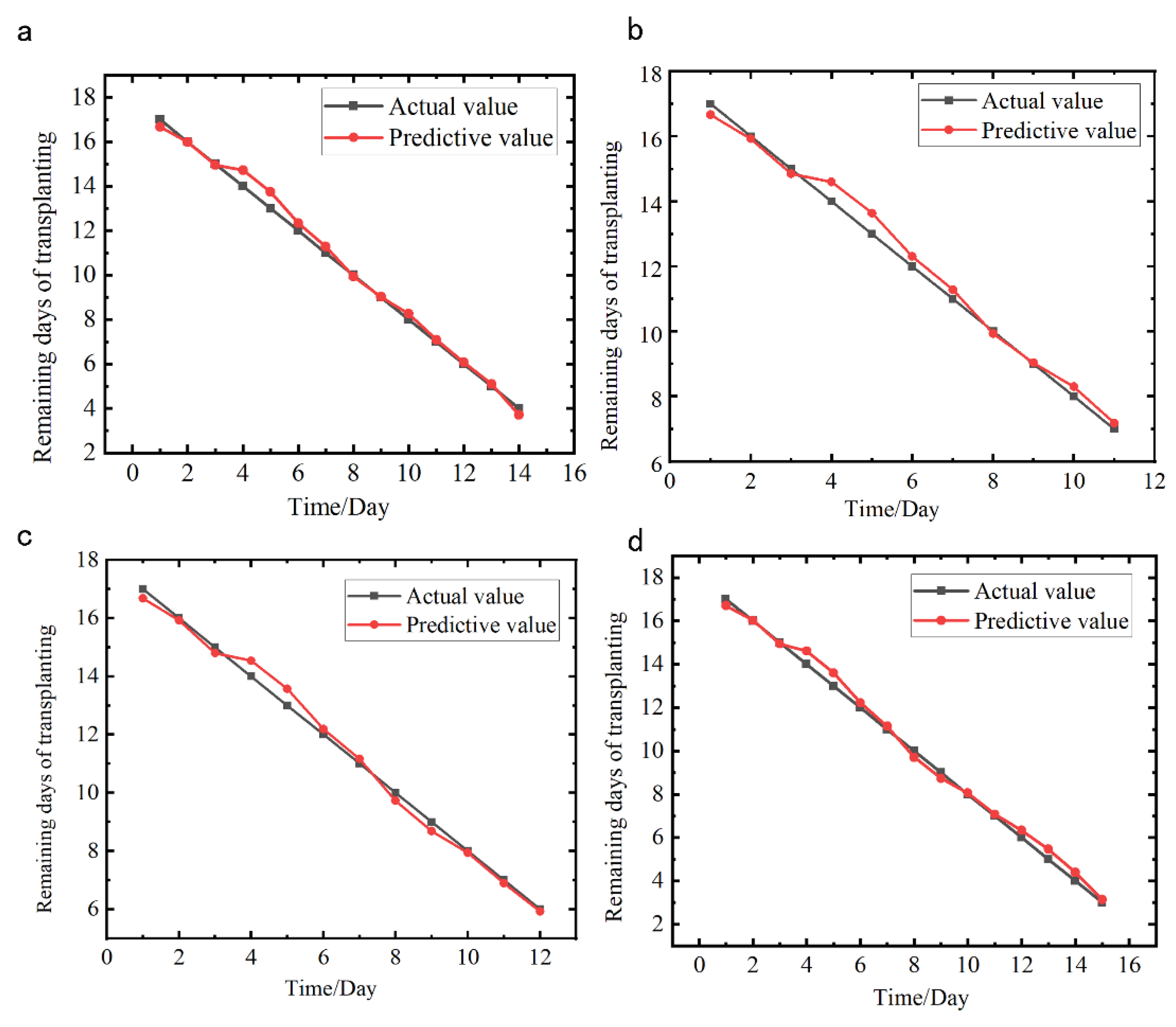
5.2. Prediction Result

This subsection contains the experimental results in three sections. First, the performance of the prediction model was analyzed to obtain the optimal parameters. Then, the attention mechanism was explored for its effect on the prediction effect. Finally, the proposed method was compared with other models to verify its feasibility.

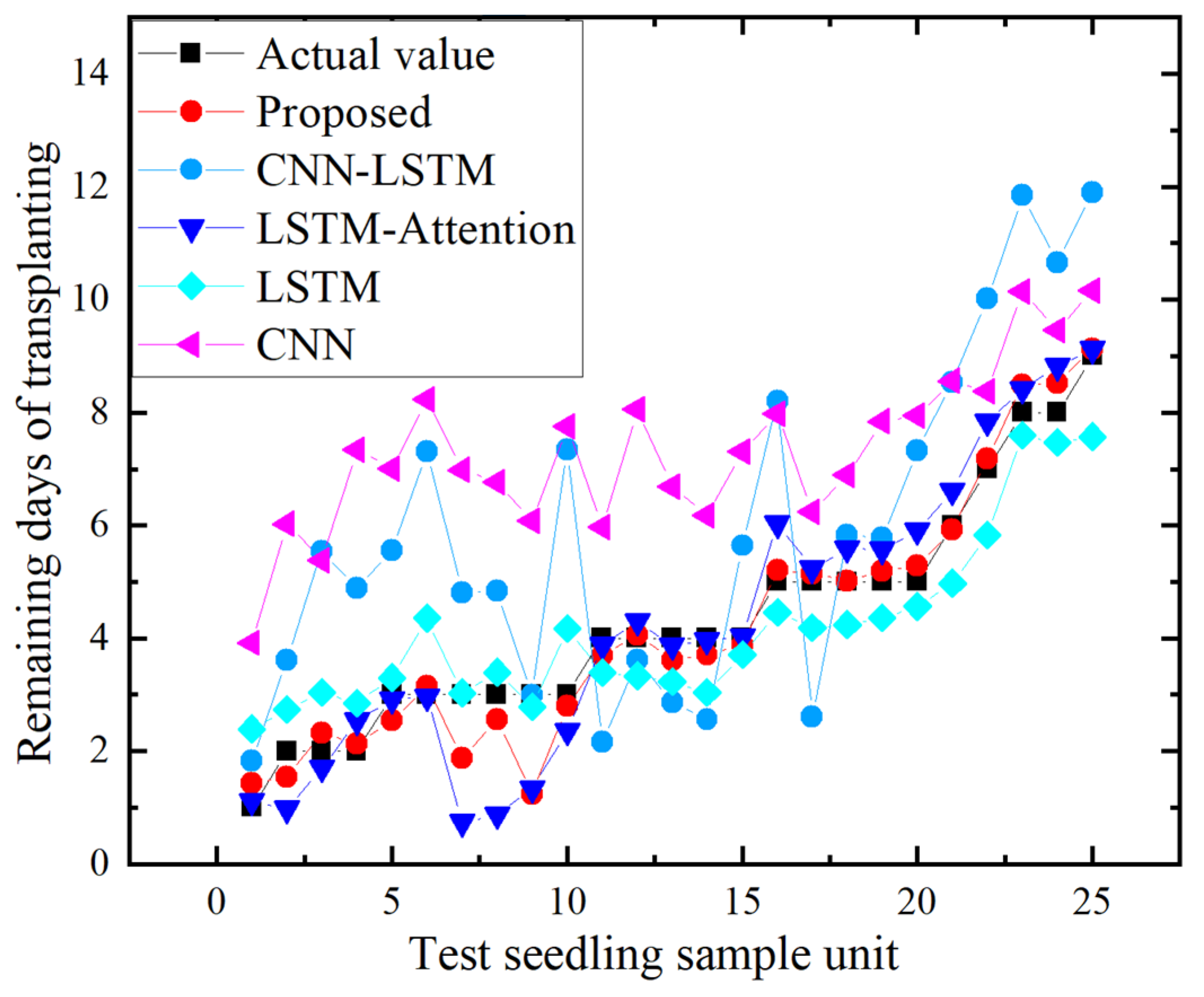
5.2.1. Performance Analysis of Predictive Models

To demonstrate the effectiveness of the proposed prediction model, the Shandong Seedling Plant dataset was taken as an example for analysis. Zhonggan 21 data were used as the training set, and purple cabbage data were used as the test set. The weights of the optimized model were updated using the adaptive moment estimation (Adam) algorithm [27]. When the validation error had no downward trend for 10 consecutive Epochs, the training process was be terminated early by Early stopping. Through multiple trainings, the optimal network parameters were obtained: learning_rate = 0.001, beta_1 = 0.9, beta_2 = 0.999, epsilon = 1 × 10⁻⁸, number of iterations, 180, and batch size, 512. To explore the influence of the number of LSTM hidden layer nodes on the learning performance of the prediction model, the number of hidden layer neurons was set to 50, 100, 150, 200, 250, and 300, and the prediction results are shown in

Table 2. The effect of the number of LSTM neurons on the prediction results.

Number of Neurons	MAE	RMSE	MAPE	SMAPE
50	0.455	0.556	0.160	0.099
100	0.356	0.507	0.157	0.082
150	1.418	1.594	0.692	0.284
200	0.404	0.673	0.286	0.097
250	0.473	0.606	0.183	0.109
300	0.484	0.706	0.277	0.127

.

When the number of neurons in the LSTM hidden layer was 100, the MAE, RMSE, MAPE, and SMAPE of the prediction model on the test set reached the minimum, as shown in Table 2. Therefore, the optimal neuron network parameter for LSTM was 100.

Figure 6 shows the prediction results of planting time for four randomly selected seedling samples on the test set. It can be seen in the figure that the DCNN model can effectively extract the detailed characteristics of seedling growth. Even if the amount of data was small at the beginning, the prediction was difficult, and the predicted value was close to the real value. As the number of days increased, the LSTM could efficiently learn the contextual relationship of time series under the guidance of the attention mechanism. The prediction model learnt different features in time and space at the same time, better fitting the real degradation curve; the prediction trend appeared stable, and the prediction accuracy of the transplanting time effectively improved. Therefore, the proposed model has strong spatial multi-dimensional feature extraction ability and learning ability of time series information.

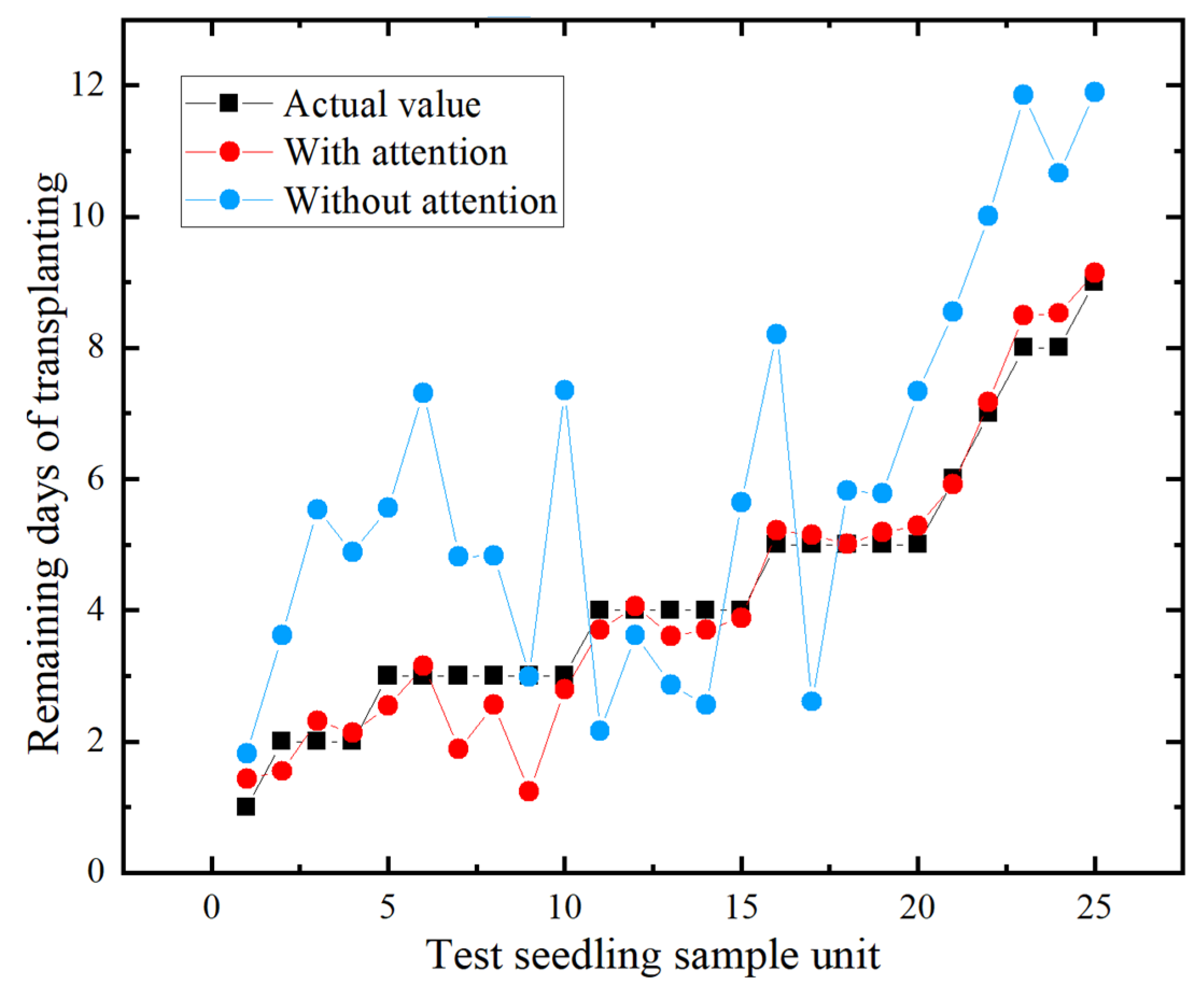
5.2.2. Effect of the Attention Mechanism on Prediction Performance

To explore the influence of the attention mechanism on the prediction effect of the model, the DCNN-LSTM model with and without the attention mechanism was considered for a comparative analysis. The simulation results are shown in Figure 7. In the figure, the abscissa represents the sample sampling number of the test set, and the ordinate represents the remaining transplanting days of the sample. The black rectangles represent the ground truth, the red dots represent the model prediction results with the attention mechanism added, and the blue circles represent the model prediction results without the attention mechanism added.

The comparison of the prediction effect of the proposed model on the test set is shown in Figure 7 that reports the prediction results of all samples on the test set sorted from small to large according to the predicted value of the remaining transplanting time. It can be seen from the figure that the attention mechanism had an important impact on the experimental accuracy. When the attention mechanism was not added to the model, the prediction result fluctuated up and down around the real value, and the change was large. After adding the attention mechanism, the prediction value converged to the direction of the real value, which greatly improved the prediction result. The predicted values of samples 7, 8, and 9 showed a certain deviation from the actual values, because the leaves of the 7th, 8th, and 9th cabbage samples fell off during the growth process, resulting in incomplete data and little information, thus increasing the difficulty of model prediction. However, the overall predicted value for the test set was consistent with the change trend of the real value, the fitting degree was good, and the proposed model showed a good prediction effect.

5.2.3. Effect of the Attention Mechanism on Prediction Performance

To prove the superiority of the proposed DCNN-LSTM model based on the attention mechanism under the same input parameters, a comparison was performed with CNN, LSTM, LSTM-Attention, and CNN-LSTM. The results are shown in

Table 3. Comparison of CNN, LSTM, LSTM-Attention, CNN-LSTM, and the proposed model for the four evaluation indicators of MAE, RMSE, MAPE, and SMAPE.

Model	MAE	RMSE	MAPE	SMAPE
CNN	3.012	3.230	0.431	0.448
LSTM	0.770	0.880	0.247	0.143
LSTM-Attention	0.621	0.870	0.387	0.138
CNN-LSTM	2.187	2.473	0.402	0.327
Proposed	0.356	0.507	0.157	0.082

and Figure 8.

The experimental results showed that the prediction accuracy of the model proposed in this paper was significantly better than that of the other four methods. The DCNN-LSTM prediction model based on the attention mechanism can not only extract high-level features of multi-dimensional data, but also have a better function fitting effect on time series prediction. Therefore, the method proposed in this paper shows strong feature learning ability in the analysis of agricultural seedling data and has broad application prospects in the task of planting time prediction.

6. Conclusions

This paper studied an intelligent prediction method with broad applicability to judge the time of cabbage transplanting based on the textual information of cabbage growth indicators and environmental factors. A prediction model combining DCNN and LSTM based on an attention mechanism is proposed that provides a new solution for predicting seedling transplanting time. In the prediction model, the DCNN extracts spatial multidimensional data features, and the LSTM performs time series prediction. The attention mechanism can focus on obtaining highly relevant information, which can guide the LSTM to fit the temporal and nonlinear relationships of complex multi-feature data more efficiently. Experiments were carried out on the data set established by the Shandong Seedling Factory, and it was concluded that the model proposed in this paper has higher prediction accuracy than CNN, LSTM, LSTM-Attention and CNN-LSTM. The practicability of the proposed method for predicting the transplanting time of cabbage can provide a theoretical basis for engineering applications.

References

1. Manchali, S.; Murthy, K.N.C.; Patil, B.S. Crucial facts about health benefits of popular cruciferous vegetables. J. Funct. Foods 2012, 4, 94–106. [Google Scholar] [CrossRef]
2. Vaishnnave, M.P.; Manivannan, R. An Empirical Study of Crop Yield Prediction Using Reinforcement Learning. Artif. Intell. Tech. Wirel. Commun. Netw. 2022, 3, 47–58. [Google Scholar]
3. Lenz-Wiedemann, V.I.S.; Klar, C.W.; Schneider, K. Development and test of a crop growth model for application within a Global Change decision support system. Ecol. Model. 2010, 221, 314–329. [Google Scholar] [CrossRef]
4. Johnson, R.; Vishwakarma, K.; Hossen, S.; Kumar, V.; Shackira, A.; Puthur, J.T.; Abdi, G.; Sarraf, M.; Hasanuzzaman, M. Potassium in plants: Growth regulation, signaling, and environmental stress tolerance. Plant Physiol. Biochem. 2022, 172, 56–69. [Google Scholar] [CrossRef]
5. Chen, Z.; Galli, M.; Gallavotti, A. Mechanisms of temperature-regulated growth and thermotolerance in crop species. Curr. Opin. Plant Biol. 2022, 65, 102134. [Google Scholar] [CrossRef]
6. Latif, M.S.; Kazmi, R.; Khan, N.; Majeed, R.; Ikram, S.; Ali-Shahid, M.M. Pest Prediction in Rice using IoT and Feed Forward Neural Network. KSII Trans. Internet Inf. Syst. 2022, 16, 133–152. [Google Scholar]
7. Drees, L.; Junker-Frohn, L.V.; Kierdorf, J.; Roscher, R. Temporal Prediction and Evaluation of Brassica Growth in the Field using Conditional Generative Adversarial Networks. arXiv 2021, arXiv:2105.07789. [Google Scholar] [CrossRef]
8. Pohan, S.; Warsito, B.; Suryono, S. Backpropagation artificial neural network for prediction plant seedling growth. In Journal of Physics: Conference Series; IOP Publishing: Bristol, UK, 2020; Volume 1524, p. 012147. [Google Scholar]
9. Taherei, G.P.; Hassanpour, D.H.; Mosavi, A.; Yusof, K.B.; Alizamir, M.; Shamshirband, S.; Chau, K.W. Sugarcane growth prediction based on meteorological parameters using extreme learning machine and artificial neural network. Eng. Appl. Comput. Fluid Mech. 2018, 12, 738–749. [Google Scholar]
10. Rimaz, H.R.; Zand-Parsa, S.; Taghvaei, M.; Kamgar-Haghighi, A.A. Predicting the seedling emergence time of sugar beet (Beta vulgaris) using beta models. Physiol. Mol. Biol. Plants 2020, 26, 2329–2338. [Google Scholar] [CrossRef]
11. Zhou, H. Rice Growth Prediction Based on Improved Elman Neural Network. Master’s Thesis, Yangzhou University, Yangzhou, China, 2019. [Google Scholar]
12. Meng, Y.R. Research and Application of Vegetable Growth Cycle Prediction Model base on Environment on the Agricultural-Cloud Service Platform. Master’s Thesis, Guizhou University, Guizhou, China, 2019. [Google Scholar]
13. Zhang, C.S.; Xu, L.J.; Li, X.L.; Li, H.; Ge, W.Z.; Liu, X.T.; Yu, X.N.; Sun, M.Y. Effects of main environmental parameters on the growth of tomato in solar greenhouse. J. China Agric. Univ. 2019, 10, 118–124. [Google Scholar]
14. Yang, L.L.; Wang, Y.M.; Dong, Q.X. Fruit growth modeling and realization for greenhouse tomato. Trans. Chin. Soc. Agric. Eng. 2013, 29, 197–202. [Google Scholar]
15. Perugachi-Diaz, Y.; Tomczak, J.M.; Bhulai, S. Deep learning for white cabbage seedling prediction. Comput. Electron. Agric. 2021, 184, 106059. [Google Scholar] [CrossRef]
16. Susilo, A.S.; Karna, N.B.A.; Mayasari, R. Bok Choy Growth Prediction Model Analysis Based On Smart Farm Using Machine Learning. eProc. Eng. 2021, 8, 1312. [Google Scholar]
17. Alhnaity, B.; Kollias, S.; Leontidis, G.; Jiang, S.; Schamp, B.; Pearson, S. An autoencoder wavelet based deep neural network with attention mechanism for multi-step prediction of plant growth. Inf. Sci. 2021, 560, 35–50. [Google Scholar] [CrossRef]
18. Singh, D.; Singh, B. Investigating the impact of data normalization on classification performance. Appl. Soft Comput. 2020, 97, 105524. [Google Scholar] [CrossRef]
19. Shin, H.-C.; Roth, H.R.; Gao, M.; Lu, L.; Xu, Z.; Nogues, I.; Yao, J.; Mollura, D.; Summers, R.M. Deep convolutional neural networks for computer-aided detection: CNN architectures, dataset characteristics and transfer learning. IEEE Trans. Med. Imaging 2016, 35, 1285–1298. [Google Scholar] [CrossRef] [Green Version]
20. Kim, P. Convolutional Neural Network. In MATLAB Deep Learning; Apress: Berkeley, CA, USA, 2017; pp. 121–147. [Google Scholar]
21. Greff, K.; Srivastava, R.K.; Koutník, J.; Steunebrink, B.R.; Schmidhuber, J. LSTM: A search space odyssey. IEEE Trans. Neural Netw. Learn. Syst. 2016, 28, 2222–2232. [Google Scholar] [CrossRef] [Green Version]
22. Vaswani, A.; Shazeer, N.; Parmar, N.; Uszkoreit, J.; Jones, L.; Gomez, A.N.; Kaiser, Ł.; Polosukhin, I. Attention is all you need. In Advances in Neural Information Processing Systems; Neural Information Processing Systems: Long Beach, CA, USA, 2017; pp. 5998–6008. [Google Scholar]
23. Wright, D.J.; Capon, G.; Page, R.; Quiroga, J.; Taseen, A.A.; Tomasini, F. Evaluation of forecasting methods for decision support. Int. J. Forecast. 1986, 2, 139–152. [Google Scholar] [CrossRef]
24. Armstrong, J.S. Evaluating forecasting methods. In Principles of Forecasting; Springer: Boston, MA, USA, 2001; pp. 443–472. [Google Scholar]
25. Makridakis, S.; Andersen, A.; Carbone, R.; Fildes, R.; Hibon, M.; Lewandowski, R.; Newton, J.; Parzen, E.; Winkler, R. The accuracy of extrapolation (time series) methods: Results of a forecasting competition. J. Forecast. 1982, 1, 111–153. [Google Scholar] [CrossRef]
26. Goodwin, P.; Lawton, R. On the asymmetry of the symmetric MAPE. Int. J. Forecast. 1999, 15, 405–408. [Google Scholar] [CrossRef]
27. Kingma, D.P.; Ba, J. Adam: A method for stochastic optimization. arXiv 2014, arXiv:1412.6980. [Google Scholar]
Figure 1. Greenhouse environment.
Agronomy 12 01504 g001
Figure 2. Schematic diagram of the 1D CNN structure.
Agronomy 12 01504 g002
Figure 3. LSTM structure diagram.
Agronomy 12 01504 g003
Figure 4. Attention network structure diagram. Green circles represent neurons.
Agronomy 12 01504 g004
Figure 5. Prediction framework diagram.
Agronomy 12 01504 g005
Figure 6. Prediction results of transplanting time for four samples in the test set. (a) Test sampling plants 5, (b) test sampling plants 10, (c) test sampling plants 15, (d) test sampling plants 20. The horizontal axis represents the time of seedling growth, and the vertical axis represents the remaining transplanting time. The black rectangles represent the true values, and the red dots represent the predicted values.
Agronomy 12 01504 g006
Figure 7. Effect of the attention mechanism on the prediction results. The horizontal axis represents the seedling sample unit of the test set, and the vertical axis represents the remaining transplanting time. The black rectangles represent the actual values, the red dots represent the predicted values with the attention mechanism added to the model, and the blue dots represent the predicted values without the attention mechanism added to the model.
Agronomy 12 01504 g007
Figure 8. Comparison of the prediction results of different models. The horizontal axis represents the seedling sample unit of the test set, and the vertical axis represents the remaining transplanting time. The black rectangles represent the actual value, the red circles represent the predicted value of the model proposed in this paper, the blue circles represent the expected value of CNN-LSTM, the purple inverted triangles represent the predicted value of LSTM-Attention, the cyan diamonds represent the expected value of LSTM, and the dark pink triangles represent the predicted values of the CNN.
Agronomy 12 01504 g008