Abstract
Precise reconstruction of the morphological structure of the soybean canopy and acquisition of plant traits have great theoretical significance and practical value for soybean variety selection, scientific cultivation, and fine management. Since it is difficult to obtain all-around information on living plants with traditional single or binocular machine vision, this paper proposes a three-dimensional (3D) method of reconstructing the soybean canopy for calculation of phenotypic traits based on multivision. First, a multivision acquisition system based on the Kinect sensor was constructed to obtain all-around point cloud data of soybean in three viewpoints, with different fertility stages of soybean as the research object. Second, conditional filtering and K-nearest neighbor filtering (KNN) algorithms were used to preprocess the raw 3D point cloud. The point clouds were matched and fused by the random sample consensus (RANSAC) and iterative closest point (ICP) algorithms to accomplish the 3D reconstruction of the soybean canopy. Finally, the plant height, leafstalk angle and crown width of soybean were calculated based on the 3D reconstruction of soybean canopy. The experimental results showed that the average deviations of the method was 2.84 cm, 4.0866° and 0.0213 m, respectively. The determination coefficients between the calculated values and measured values were 0.984, 0.9195 and 0.9235. The average deviation of the RANSAC + ICP was 0.0323, which was 0.0214 lower thanthe value calculated by the ICP algorithm. The results enable the precise 3D reconstruction of living soybean plants and quantitative detection for phenotypic traits.
1. Introduction
Soybean is an important economic crop that occupies an important position not only in China’s national economic development but in the world’s food and oil crops [1]. Soybean is grown on a large area in the northern Heilongjiang Province of China, accounting for more than half of the province’s total area, but the overall yield level is not high because of environmental constraints, and soybean varieties in the northern Heilongjiang Province are of a single type, so the yield traits are not fully consistent with other regions [2]. Plant height determines plant competition and access to nutrients, which in turn affect the yield of soybean [3,4]. The angle of the petiole directly affects the plant’s absorption of light energy [5], and changes in the spatial distribution of the crown width can greatly influence the light energy utilization of the soybean plant, which also affects the yield of soybean [6]. Traditionally, the measurement of morphological parameters in soybean plants has been carried out manually or with two-dimensional images. Manual measurements are slow, costly and subjective [7,8] and can be damaging to the plant, making them unsuitable for continuous measurement of soybean plants [9]. Measurements based on 2D images are often less accurate because of interplant shading and are even unsuitable for measuring morphological parameters such as canopy width because of dimensional limitations [10]. Therefore, accurate acquisition of the 3D point cloud of the soybean canopy and calculation of phenotypic traits such as plant height, leafstalk angle and crown width are necessary for selecting and breeding excellent soybean varieties.
In recent years, 3D reconstruction technology has been used in a wide range of areas in agriculture, throughout the entire agricultural production process, such as seed identification, crop growth simulation, growth monitoring and final harvesting, as well as the testing and grading of agricultural products. Plant genomics are developing in the direction of intelligence, visualization and digitization. Three-dimensional reconstruction is an important part of plant digitalization research. It can be used not only to explore the growth and development patterns of plants by simulating the effects of environmental changes on the plant 3D model but to digitize the phenotypic characteristics of plants so that their growth states can be systematically analyzed to guide agricultural production [11]. The PMD camera can acquire both color and deep images. It is relatively cheap and portable, with a high framerate, but the low resolution and sensitivity to external light limits its further application [12,13]. Although laser scanning technology can establish the 3D structural form of an object more accurately and better overcome the influence of light variation, much human interaction is required when acquiring data. In addition, slow acquisition rate, data redundancy and high price restrict its use [14,15,16,17]. The Kinect V2 camera was used to acquire the raw 3D point cloud of an apple tree in binocular view Although the 3D point cloud morphological structure of the apple tree with color information was reconstructed and the algorithm stability was verified by analyzing the errors of several alignment methods [18], the binocular vision was not able to well reconstruct the full range of structural features of the apple tree. On the VC platform, a virtual wheat-growth system was constructed using OpenGL that well simulated the morphological features of wheat and extended to the full growth cycle of individual wheat plants [19], but the virtual 3D structural morphology could not completely represent the physical plant, much less cover all the conditions of the physical plant. Wu Dan et al. used a Kinect camera to obtain multiview images of rice and 3D reconstructed the rice plants by the contour projection and inverse projection methods [20]. Zhu Binglin et al. performed individual and group 3D reconstructions of maize and soybean plants at different growth stages in the field and manually measured leaf length and maximum leaf width. These measurements were compared with the reconstructed results to assess the accuracy of the 3D reconstruction [21].
In response to the problems of the fact that the full-view 3D structural morphology of the soybean canopy cannot be obtained from single and dual views, the low efficiency of manual acquisition of plant phenotypes and the high price of high-end devices, three Microsoft Kinect 2.0 cameras were chosen as the experimental equipment for acquiring data in this study because of fast, stable, high-cost performance and high image resolution [22]. In this study, two varieties of soybean, Heihe 49 and Suinong 26, were used as research objects, and the point clouds of the soybean canopy were obtained by photographing several groups of soybean plants at different growth periods. The point clouds were then accurately aligned using the ICP algorithm to achieve the fusion of the soybean canopy point clouds at different angles. On the basis of the reconstruction results, the phenotypic traits of the soybean canopy were calculated.
2. Soybean Canopy Image Acquisition
A large amount of data on soybeans were acquired at different growth stages from June 2019 to September 2021 using three Kinect v2 sensors. Each sensor was fixed on a tripod, and a potted soybean plant was placed on a bench so that it could be presented within the best view field. The study was carried out with two different varieties of soybean, Suinong 26 and Heihe 49, at four growth stages, the flowering, podding, filling and mature stages. The distance between the camera and the potted plant changed as the soybeans grew differently at each stage. From June to July, the soybean plants were generally under 30 cm tall, and the camera height was set at around 60 cm, with the camera lens at around 60 cm from the potted plant. From August to September, the soybean plants were generally 30–70 cm tall, with the camera set at around 75 cm and the camera lens around 95 cm from the pot. The three sensors were at about 120° angles of from each other and at the same level so that a full range of three-sided point cloud data could be obtained from the horizontal plane of the soybean canopy. The sensors themselves were kept horizontal and adjusted to a level to avoid distortion of the images. The acquisition schematic is shown in Figure 1a. The experimental scene is shown in Figure 1b. The acquired color and depth images of the horizontal all-round triple view of the soybean plants are shown in Figure 2.
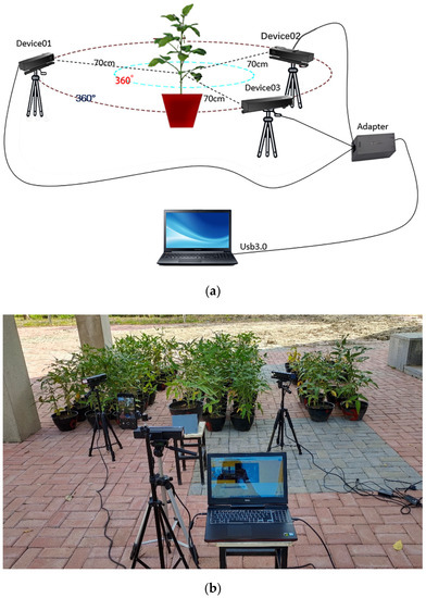
Figure 1.
Schematic and scene of soybean canopy acquisition: (a) acquisition schematic; (b) experimental scene.
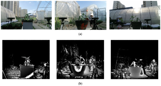
Figure 2.
Color and depth maps of soybean plants in three views: (a) three views of the color image; (b) three views of the depth image.
3. Overall Framework for 3D Reconstruction of Soybean Canopy and Calculation of Phenotypic Traits
Using cold region soybean plants as the experimental objects, the multivisual acquisition system was used to obtain multisource data on the soybean canopy from three viewpoints. First, the point clouds of the soybean canopy were extracted from the background using the conditional filtering algorithm. Second the extracted 3D data was denoised by the KNN algorithm. Third, the RANSAC method was used to perform rough registration between viewpoint 1 and the main viewpoint and between viewpoint 2 and the main viewpoint. In addition, the wrong matching points in the matching point set were removed for fine matching. Finally, the 3D structure of the soybean canopy was reconstructed. Phenotypic traits including plant height, leafstalk angle and crown width of the soybean canopy were calculated on the reconstructed canopy structure. The run time and the distance to the nearest point after point cloud matching were compared between the traditional ICP and the proposed algorithm to verify the accuracy of the latter. The phenotypic traits were calculated and compared with the measured values using mean error and linear correlation to prove the feasibility of the proposed algorithm. The overall framework is shown in Figure 3.
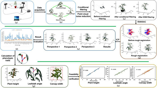
Figure 3.
Overall framework for 3D reconstruction of soybean canopy and calculation of phenotypic traits.
4. Preprocessing of Point Cloud
4.1. Point Cloud Filtering and Noise Reduction
The Kinect V2 sensor can acquire depth and color images of the target object. The spatial mapping relationship between the color image and the depth image can be obtained through a mapping function in the Kinect V2 development kit. After mapping of the depth image, the color information can be obtained, and then the point cloud coordinates in the world coordinate system can be acquired through the position and angle information. However, there is a large amount of background information, and there are many noises in the raw point cloud, and the spatial coordinate position and shape of the target object are very unclear, so the background and noise need to be removed as a priority.
The point cloud was first filtered through a conditional filtering algorithm to suppress redundant background information. The conditional filtering selected the point clouds by setting filtering conditions, leaving the point clouds when they were within the set range and discarding them if they were not. As the first step in point-cloud processing, the filtering process directly affected the effectiveness of subsequent point cloud matching. Only by filtering out noise points, outliers and voids in the filtering process could subsequent steps such as registration, feature extraction and reconstruction be performed. Each point in the point cloud dataset expressed a certain amount of information. The denser the points in a certain area, the greater the amount of useful information. The amount of information in isolated outliers was small, and the amount of information expressed could be ignored. In the point cloud information, separate thresholds were set for , and . The range of values for these three coordinates depended on the point cloud data, as soybean growth conditions varied from period to period. The ranges of , and during the flowering and podding stages were from −0.5 to 0.5, from −0.2 to 0.3 and from 0.2 to 1.2, respectively. The ranges of , and during the filling and maturity stages were from −0.5 to 0.5, from −0.4 to 0.6, and from 0.6 to 1.6, respectively. The comparison results before and after the conditional filtering are shown in Figure 4.
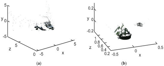
Figure 4.
Comparison before and after point cloud conditional filtering: (a) before conditional filtering; (b) after conditional filtering.
As can be seen in Figure 4b, the shape and position of the conditionally filtered target point cloud was more distinct and freer from background interference, reducing the workload and time for subsequent point cloud noise reduction. After conditional filtering background information, it contained a small number of noisy points and outliers, which were often caused by external interference and measurement errors during data acquisition. In order to acquire an effective point cloud without affecting the plant boundaries, the KNN limit filtering method was chosen to eliminate the isolated noise points.
The core of the KNN was to determine whether two vectors were similar by the distance between them. Generally, points similar to the feature points were selected. If the selected points had low similarity, then the most similar of them was the nearest neighbor matching point. For distance measurement, there are many distance measurement methods, but the most commonly used is Euclidean distance [23]. The Euclidean distance is defined as Equation (1):
where and are -dimensional vectors.
Let be a set of point clouds and be a point in the point set . The nearest neighbors of in were called k-nearest neighbors of , denoted as . If the distance between the measured points and the selected point was small and similar, then the most similar point was the nearest neighbor matching point of .
The steps of the KNN filtering can be summarized as follows:
- Read in the 3D coordinate values of the point cloud, establish a K-dimensional tree, form topological relationships between points, organize and manage point cloud data and then find nearest neighbor points for each point, storing the nearest neighbor distance [24].
- Extract the nearest neighbors of each point on the point cloud on the basis of the K-dimensional tree structure.
- Use Equation (1) to calculate the distance between each point on the point cloud and its nearest neighbors, and then calculate the sum of these distances, as shown in Equation (2):
- Calculate the average, , of the distances, as shown in Equation (3):
- If the distance of the nearest neighbors of a point is greater than a certain threshold , determine it to be an anomaly or a noisy point [25]. In this study, the threshold was chosen to be 0.01, and the value of was taken to be 8. The same treatment was done for the three-sided point cloud of each potted plant at different growth stages.
4.2. Analysis of Filtering Noise Results
In order to verify the effectiveness and denoising accuracy of the above filtering methods, filtering experiments were carried out on soybean plants in different growth stages. The conditional filtering results of the flowering, podding, filling, and maturity stages were shown in Figure 5a, and the noise filtering results based on KNN algorithm were shown in Figure 5b.
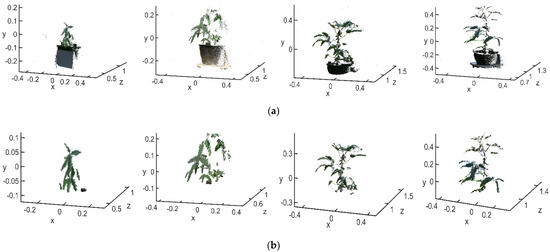
Figure 5.
Point cloud after noise reduction: (a) before k-nearest neighbor filtering; (b) after k-nearest neighbor filtering.
In Figure 5a, the number of points in the raw point cloud at the flowering stage was 42,664, and the number after filtering was 22,723; 19,941 background point clouds were removed. The number of points in the raw point cloud at the podding stage was 38,442, and the number after filtering was 26,618; 11,824 background point clouds were removed. The number of points in the raw point cloud at the filling stage was 58,527, and the number after filtering was 14,985; 43,542 background point clouds were removed. The number of points in the raw point cloud at mature stage was 56,231, and the number after filtering was 12,468; 43,763 background point clouds were removed. The percentages of background points removed were 46.7%, 30.8%, 74.4% and 77.8%, respectively. The numbers of background point clouds were related not only to the performance of the camera itself but to the distance from the target object to the camera. During flowering and podding stages, the soybean plants were smaller in height and therefore closer to the camera. Therefore, the number of point clouds of the target object was higher, and the number of background point clouds was lower, compared with the total number of point clouds acquired. During the filling and mature stages, the soybean plant was taller and further away from the camera; thus, the number of point clouds of the target object was smaller compared with the total number of point clouds acquired. In addition, the number of background point clouds was larger in the later stages, so the background point cloud removal rate was smaller during the flowering and podding stage than during the filling and mature stages.
To further analyze the performance of the KNN denoising algorithm in this paper, four groups of denoising accuracy were obtained by counting the point cloud size, denoising accuracy and runtime. The denoising accuracy was defined by Equation (4):
where was the number of point clouds before noise reduction and was the number of point clouds after noise reduction.
The result after noise reduction is shown in Figure 5b. To prevent the reconstruction from falling into local optima, the point cloud of the pot was not included in the matching, so it also needed filtering out. Therefore, the number of point clouds before KNN filtering during the flowering period was 4853, and the number of point clouds after KNN filtering was 4309, with 544 noise points removed. The number of point clouds before k-nearest neighbor filtering at the podding stage was 11,275, and the number after KNN filtering was 9977, with 1298 noise points removed. The number of point clouds before KNN filtering at the filling stage was 10,479, and the number after KNN filtering was 10,215, with 264 noise points removed. The number of point clouds before KNN filtering at the mature stage was 9042, and the number after KNN filtering was 8673, with 369 noise points removed. The overall marginal detail of the canopy was preserved intact. In regard to the effectiveness of the KNN algorithm, the numbers of points were reduced to 91.2%, 87.4%, 96.8% and 97.1% of the numbers before KNN filtering for each growth stage. Although the percentages of reduced points were not high, they represented only close, isolated noise points. As shown by counting the size of the number of point clouds and the denoising accuracy under the four datasets, the average denizen accuracy of the point cloud data for the four growth stages was above 93%. As can be seen from comparison of the results (Figure 5), the KNN used here was able to perform outlier removal over a large range and high noise, effectively retaining sharp and edge features as well as stem detail features in the raw point cloud. Thus, KNN was an effective point cloud denoising algorithm.
5. Point Cloud Registration
The goal of registration was to find the relative positions and orientations of separately acquired views in a global coordinate frame such that the intersection regions between them overlapped completely. The registration algorithm often used in 3D registration is the iterative closest point (ICP) algorithm [26]. However, because of defects in this algorithm, the final iterative result may fall into local optimization, resulting in registration failure. Therefore, in order to improve the accuracy of registration results, it was necessary to provide better initial values of the translation and rotation matrixes; that is, rough registration was performed first.
5.1. Rough Registration of the Point Cloud
Rough registration refers to the registration of point clouds when the relative pose of point clouds is completely unknown; it can provide a good initial value for fine registration. RANSAC is an iterative algorithm to correctly estimate the parameters of the mathematical model from a set of data containing “outliers”. A fundamental assumption of RANSAC is that the data are made up of “interior” and “exterior” points. The “interior points” refer to the data that make up the parameters of the model, while the “outer points” generally refers to noise in the data, such as mismatches and outliers in the estimated curve. RANSAC also assumes that, given a set of data with a small number of “interior points”, there is a program that can estimate a model that fits the “interior points”.
For the accuracy and effectiveness of point cloud registration, the feature point set was selected. The change degree of the normal vector of a point on a region reflected the bending degree of the region [27]. A low degree of variation in a normal vector indicated that the area near the corresponding point was relatively smooth, and thus fewer points could be sampled in this area. On the contrary, if the degree of variation in a normal vector was large, the change in its nearby area was obvious, and more points needed sampling to describe the characteristics of this area. The arithmetic mean of the angle between the normal vector at a point in the point cloud and the angle between the normal vectors of its nearest neighbors was defined as follows:
where is the arithmetic mean and is the angle between the normal vector at a point and the normal vector at the th nearest neighbor.
According to this definition, the larger the feature degree was, the greater the variation was in the undulation of the region, so this feature degree could be used to extract the feature points above the mean value in the point cloud. The values for the flowering, podding, filling and mature stages were 8, 8, 10 and 10, respectively. The raw point clouds of view 1, view 2 and the main view for the four growth stages are shown in Figure 6, and the screening results are shown in Figure 7.
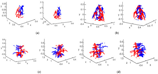
Figure 6.
Raw 3D point cloud: (a) flowering stage; (b) podding stage; (c) filling stage; (d) mature stage.
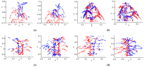
Figure 7.
Points with above-average eigenvalues: (a) flowering stage; (b) podding stage; (c) filling stage; (d) mature stage.
After filtering by the value of , there were 1728 points with above-average flowering stage characteristics in the main view, 1654 in view 1 and 1800 in view 2. The numbers of points with above-average podding stage characteristics were 5553 in the main view, 4634 in view 1 and 4355 in view 2. The numbers of points with above-average filling stage characteristics were 3725 in the main view, 1990 in view 1 and 4574 in view 2. The numbers of points with above-average mature stage characteristics were 3307 in the main view, 2403 in view 1 and 4510 in view 2. As shown in Figure 7, the soybean canopy in the flowering and podding stages had a more obvious growth trend, and the overall morphology of the canopy was more variable, so the number of points with above-average characteristic degrees in the podding stage was 9360 more than that at the flowering stage. However, at the filling and mature stages, the biggest changes were in the size of the pod morphology, the canopy morphology and phenotypic traits. Thus, from the overall perspective, the number of points with above-average characteristic degrees in the filling stage was only 69 more than that at the maturity stage, and the number of point clouds in the two periods was almost the same. The raw point clouds were filtered by the mean value of the characteristic degree, and the preserved point clouds gave a general picture of the canopy characteristics and morphology of the soybean plants.
A threshold, , was set. Points with were kept, as the more undulating point clouds were more representative of the object’s features. Of all the points in the k-nearest neighborhood, the point with the largest was retained as the feature point. took a relatively small value and would retain more detailed information about the raw point cloud. Since the s of the 3D point clouds were different for each growth stage, the mean eigenvalues of the main view were 0.7887 at the flowering stage, 0.7645 for view 1 and 0.7587 for view 2; 0.6965 at the podding stage, 0.6839 for view 1 and 0.6979 for view 2; 0.8544 at the filling stage, 0.8892 for view 1 and 0.8407 for view 2; and 0.8509 at the mature stage, 0.8954 for view 1 and 0.8505 for view 2. The results of the feature point set selection are shown in Figure 8.
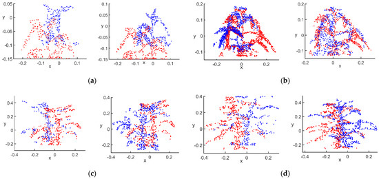
Figure 8.
Selection of feature point sets: (a) flowering stage; (b) podding stage; (c) filling stage; (d) mature stage.
After filtering according to the value of , the set of feature points in the main view at the flowering stage had 290 points; view 1 had 293 points, and view 2 had 289 points. The set of feature points at the podding stage had 977 points in the main view; view 1 had 837 points, and view 2 had 721 points. The set of feature points at the filling stage had 511 points in the main view; view 1 had 267 points, and view 2 had 623 points. The set of feature points at the mature stage had 571 points in the main view; view 1 had 328 points, and view 2 had 601 points. There were significantly fewer points in the feature point set than after filtering using the mean value, because the feature points were more representative of the core shape of the entire point cloud, which had a higher degree of similarity for matching. This allowed for more targeted matching of subsequent point pairs. The reduction in the number of points also reduced the number of incorrectly matched point pairs to some extent, providing better conditions for initial feature point matching.
Some points in the point cloud overlapped; for some points in the source point cloud , the target point cloud had no matching points for them. We thus chose an appropriate threshold . When the distance between feature vectors was less than , these feature point pairs were not involved in matching. The remaining matching point pairs greater than the distance were used as the initial matching point pairs. The values for the four growth stages(flowering, podding, filling and mature stages), were 0.2, 0.2, 0.5 and 0.5, respectively. The selection results are shown in Figure 9. Since it was difficult to find the exact corresponding points for two discrete point clouds, the correct matching points here were only approximate corresponding point pairs.
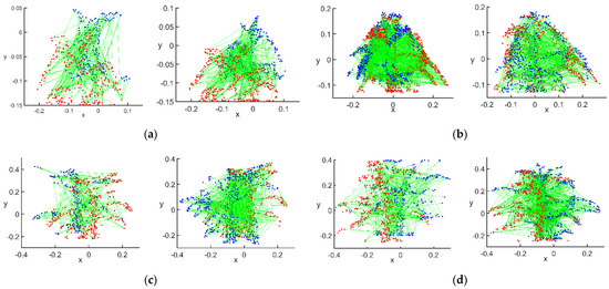
Figure 9.
Initial matching effect of feature points: (a) flowering stage; (b) podding stage; (c) filling stage; (d) mature stage.
Based on the value of , the initial number of point pairs matched between the main view and view 1 at the flowering stage was 290, and that between the main view and view 2 was 289. The initial number of point pairs matched between the main view and view 1 at the podding stage was 439, and that between the main view and view 2 was 388. The initial number of point pairs matched between the main view and view 1 at the filling stage was 256, and that between the main view and view 2 was 511. The initial number of point pairs matched between the main view and view 1 at the mature stage was 280, and that between the main view and view 2 was 503. The purpose of using points with a point spacing greater than as the initial matching points was to maximize the fusion of the overall point clouds of view 1 and view 2 with the main view. Pairs of points with a point spacing less than were considered as already matched points.
The initial set of matched point pairs was equal between any two point-pairs according to the distance invariance of the rigid transformation. The distance invariance is shown in Equation (6):
where , , , . The appropriate was chosen for each pair. For each matched point pair , the number k of point pairs in the point set other than it that satisfied the rigid distance constraint was calculated, and a point pair in the matched point set satisfied Equation (7).
Then, the point pair was denoted as the distance-constrained point pair relative to the point pair . In this paper, the values of for the four growth stages (flowering, podding, filling and mature stages), were taken as 0.1, 0.13, 0.3 and 0.3, respectively. A certain number of correctly matched point pairs existed among the matched point pairs obtained from the initial matching, and in general, the number of point pairs obtained from correctly matched point pairs that met the distance constraint was relatively large. The value of was calculated, and the top point pairs were selected using the binomial tree rule. Then, the set of matched point pairs was sorted according to the value of from largest to smallest. The feature matches for the four stages after the point cloud was filtered by the rigid invariance constraint are shown in Figure 10.
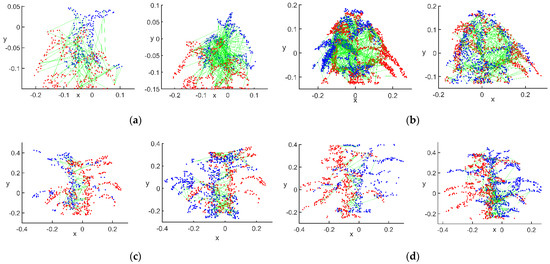
Figure 10.
Matching effect after filtering for rigid invariant constraints: (a) flowering stage; (b) podding stage; (c) filling stage; (d) mature stage.
After filtering by the rigid invariance constraint, there were 116 matching point pairs between the main view and view 1 and 101 matching point pairs between the main view and view 2 at the flowering stage. There were 350 matching point pairs between main view and view 1 and 335 matching point pairs between the main view and view 2 at podding stage. There were 101 matching point pairs between main view and view 1 and 377 matching point pairs between main view and view 2 at the filling stage. There were 190 matching point pairs between the main view and view 1 and 385 matching point pairs between the main view and view 2 at the mature stage. This step reduced the number of matched point pairs for the initial match to some extent. The main purpose of this step was to remove radial and lateral aberrations in the images and point cloud information obtained by using different KinectV2 sensors at different angles. This distortion caused the distance information of the corresponding point pairs at different angles to deviate, and the accuracy of this distance parameter directly affected the accuracy of the 3D reconstruction, and thus the judgement of the RANSAC algorithm on the correct matching point pairs.
The calculation of the rigid body transformation matrix required at least three pairs of matched points in 3D space that were not colinear ( was an adaptive variable). Three points out of were randomly selected as a sample and considered as normal matching point pairs. The rigid body transformation matrix was calculated to determine whether the remaining point pairs were the correct matching point pairs under . Then, three more points were selected at random up to the upper limit, and the rigid transformation matrix with the highest number of internal points was taken as the correct transformation matrix, with the internal points as the final matching point pairs. Based on the correct set of matching points obtained, the initial alignment parameters obtained were calculated using the four-element method. The rotation matrix R and translation matrix are shown in Equation (8):
The point cloud after the RANSAC process is shown in Figure 11.
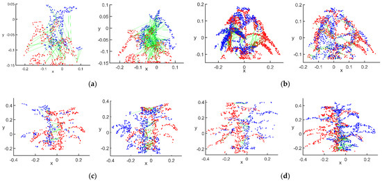
Figure 11.
Matched point pairs after RANSAC processing: (a) flowering stage; (b) podding stage; (c) filling stage; (d) mature stage.
The correct values of were tested using the RANSAC algorithm as follows: at the flowering stage, 81 matching point pairs were screened between the main view and view 1, and 70 matching point pairs between the main view and view 2. At the podding stage, 181 matching point pairs between the main view and view 1, and 175 matching point pairs between the main view and view 2, were screened. At the filling stage, 33 matching point pairs between the main view and view 1, and 264 matching point pairs between the main view and view 2, were screened. At the mature stage, 125 matching point pairs between the main view and view 1, and 264 matching point pairs between the main view and view 2, were screened. As can be seen in Figure 10, after processing via the above algorithm, the final matched point pairs and the point pairs in their neighborhoods were the best conditions for the rotation–translation transformation of the two point clouds during rough registration. However, in Figure 10c, the point cloud at the filling stage showed a many-to-one matching relationship after the above matching steps, which was mainly distributed on the matching of stem points because of the accuracy of the Kinect sensor and the variation of different camera angles.
5.2. Analysis of Rough Registration Results
The results of initial matching of the main view with views 1 and view2 at the flowering, podding, filling and mature stages are shown in Figure 12.
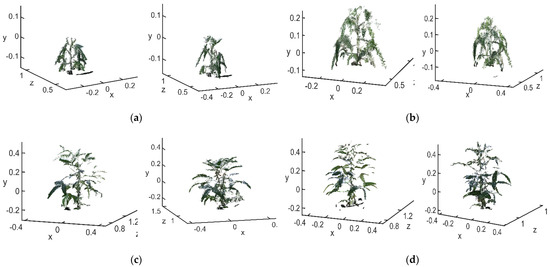
Figure 12.
Rough registration results: (a) flowering stage; (b) podding stage; (c) filling stage; (d) mature stage.
As can be seen in Figure 12, the spatial positions of views 1 and 2 changed to varying degrees compared with the original point cloud, except for the position of the main viewpoint, which remained unchanged. Both had fused parts of the point cloud with the main viewpoint. The improved registration ranges of the four growth stages, flowering, podding, filling and mature, were 43.1–48.31%, 36.4–40.76%, 31.5–39.66% and 43.8–60.1%, with average increases in registration of 45.9%, 37.25%, 37.1% and 56%, respectively. The improvement in the match rate was more obvious. Although the conditional filtering of matched point pairs using the RANSAC matching did not guarantee that all incorrectly matched point pairs would be eliminated, the algorithm provided a better initial point cloud bit pose for subsequent fine matching. Thus, the above method not only eliminated some of the mismatched point pairs but yielded the optimal quadratic rotation–translation matrix. The above experimental results showed that the method had good robustness to point cloud noise and outliers. To a certain extent, it provided a good initial point cloud for the ICP, reduced the runtime of the ICP, avoided the generation of local optimal solutions and improved the accuracy of registration, providing more details of plant morphology for subsequent 3D reconstruction.
5.3. Accurate Registration of the Point Cloud
The purpose of accurate registration was to minimize the spatial position difference between point clouds based on rough registration. The basic principle of the traditional ICP algorithm is the optimal registration method based on the least squares, and the point clouds were paired according to the spatial geometric transformation. The corresponding points were matched to the set and then combined with the transformation matrix to transform. Matching to the corresponding points continued, and this process was iterated until the result met the convergence requirements to obtain the correct matching result. By using this algorithm, the accuracy of point cloud matching was higher, but the operation speed and accuracy of the algorithm depended largely on the initial position of the two given point clouds and the number of point clouds. The traditional ICP algorithm could accurately match two point-clouds when there was an envelope relationship between the two clouds and their positions were close to each other. Point clouds shot from different angles only partially overlapped, however, and their spatial positions were quite different. The traditional ICP algorithm generates local optima because of improper selection of initial values. Therefore, this study first used the RANSAC algorithm to first perform rough registration, which provided better initial values for the ICP. Assuming that there was an origin point cloud and a target point cloud , there was not a one-to-one correspondence between and coordinate points, and the numbers of elements did not have to be the same. Given , the registration process was to select the target point cloud, consider the points in the raw point cloud as the control points and compute the nearest points between and to obtain the rotation and translation transformation matrices between the two point clouds to achieve the effect of fusing stitching. When selecting the control points, in order to get the nearest points of all points in the raw point cloud in the target point cloud , all points of the view 1 and 2 point-clouds were used as control points, and the nearest points of each point in views 1 and 2, respectively, were found in the main view.
First, the center of the two point-clouds were calculated. This was an imaginary point where the mass of the object was concentrated, and its coordinates were obtained by calculating the average of the coordinate values of all points in the point cloud [28]. Each point in the point cloud was subtracted from the coordinates of the center of mass point and finally resaved as a new point cloud datum for the next step of singular value decomposition (SVD) to find the transformation matrix. The equation for finding the coordinates of the center of the point cloud is shown as Equation (9).
where is the number of point clouds.
The SVD algorithm was used to solve the rotation and translation matrices. Assuming that was a matrix of , the SVD of the matrix is defined by Equation (10):
where is a matrix of ; is a matrix of with all zeroes except for the elements on the main diagonal, which were singular; was a matrix of ; and and satisfied and . In addition, was a unitary matrix of order .
The matrix multiplication of and yielded a square matrix of . After agent decomposition, the eigenvalues and eigenvectors obtained satisfied Equation (11):
where the eigenvalues of the matrix and the corresponding eigenvectors of were obtained, and all the eigenvectors of formed the matrix , = 1, 2, …, .
The matrix multiplication of and yielded a square matrix of . After agent decomposition, the eigenvalues and eigenvectors obtained satisfied Equation (12):
where = 1, 2, …, . The eigenvalues of the matrix and the corresponding eigenvectors were obtained. The matrix in Equation (10) was formed by all the eigenvectors of the matrix . At this point, both the matrices and were derived. The transformation relationships and between the two raw point clouds are shown in Equations (13) and (14), respectively:
In the process of matching, the accuracy of each iteration was calculated using the variable, which described the size of the gap between the predicted and true values of the model. The distance between each corresponding control point of the two point- clouds was calculated, and the maximum value of the distance was taken. Thus, the number of iterations was 100, which was calculated by Equation (15). The estimated values of standard deviation of error for each iteration were stored using the value of as the judgment condition. There were two conditions to stop iteration: (1) and the number of iterations < 100; (2) and the number of iterations ≥. As for why was taken as 0.0000001, if the value of was too small, the 100 iterations would be far from enough to achieve the expected effect, and in the process of iteration, it would be easy to miss the current optimal solution; this would be time consuming and of little practical value. If the value of was large, the iteration would stop before the optimal solution reached, and the expected effect would not be achieved. After several trials, 0.0000001 was finally chosen as the judgment condition. The calculation method is shown in Equation (16):
where, the initial value of E was the maximum value of the corresponding control point distance, was the number of iterations, was the number of control points, was the distance value of the centroid generated after each iteration and and changed as shown in Figure 13.
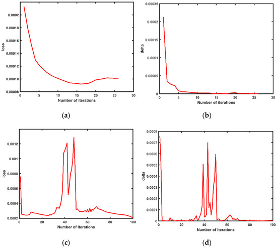
Figure 13.
Two variations of error parameters in the point cloud matching process. (a) The loss changed during the matching of the main view with the point cloud from view 1; (b) the delta changed during the matching of the main view with the point cloud from view 1; (c) the loss changed during the matching of the main view with the point cloud from view 2; (d) the delta changed during the matching of the main view with the point cloud from view 2.
It can be seen from Figure 13 that when the main view point cloud was matched with point cloud 2, although it did not reach the threshold range after 100 iterations, the values of and showed a trend of convergence; converged to 0.000001149 and converged to 0.0002075. The fluctuations that appeared in the middle 30–50 iterations were the cases in which ICP fell into the local optimal solution. In Figure 13c,d, the three peaks of were 0.0005077, 0.000699 and 0.0005949, and the two valleys were 0.000035 and 0.00005596, while the two peaks of were 0.001212 and 0.001285 and the one valley was 0.0005125. These peaks and valleys showed that in the process of matching the point cloud with point cloud 2 in the whole main point of view, the algorithm fell into the optimal solution twice, which was caused by the differences in the overall contour characteristics and quantities of the two point clouds. In the process of calculating the nearest point distance, many erroneous points were regarded as the nearest points in space, and the complexity of the spatial distribution of the point cloud made the calculation of the nearest points have more points corresponding to one point, which in turn made the calculation of the quadratic rotation–translation matrix reach a local optimum or an erroneous solution.
Assuming that the 3D coordinates of the th corresponding point in the origin cloud and the target point cloud were and , respectively, the matching point pair was defined as the closest point in the two point clouds, and the error was defined as the distance of the matching point pair. A certain point was read from the origin in point cloud , each point in the target point cloud was checked to find its distance from P in a distance array, and the smallest element in the distance array was recorded as the min-distance. The corresponding 3D coordinate points in and made up a matching point pair, and the min-distance was the matching error. The smaller the error, the higher the accuracy of the stitching. In the ideal case, when the distances between the closest point pairs were all zero, the resulting transformation matrix had error-free stitching [29].
The error calculation method is shown in Equation (17):
The raw point cloud before matching is shown in Figure 14a. The 3D point clouds in each stage are the main view, view 1 and view 2. The final matching result is shown in Figure 14b.
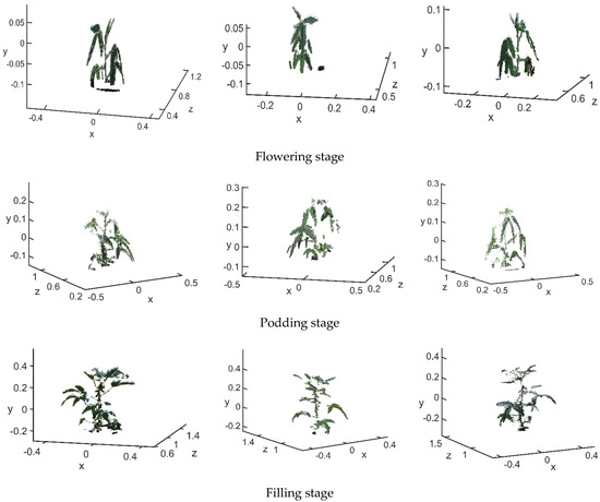
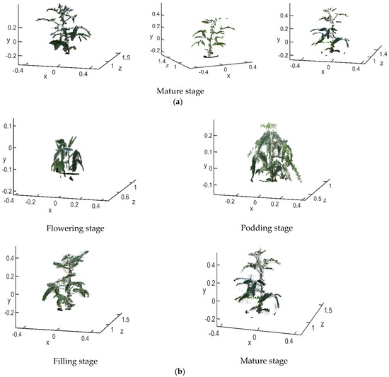
Figure 14.
Point cloud registration (a) before registration (b) after reconstruction.
After being registered by the RANSAC + ICP algorithm, the average distances between the closest points in the soybean canopy point clouds for the four growth stages, flowering, podding, filling and mature, were 0.00485 m, 0.0095 m, 0.0115 m and 0.0101 m, respectively. The average distances between the closest points processed only by the traditional ICP algorithm were 0.05135 m, 0.0119 m, 0.0879 m and 0.01845 m, respectively; the matching accuracy was improved by 0.0465 m, 0.0024 m, 0.0764 m and 0.00835 m, respectively. The number of point clouds in the flowering stage was less than 10,000, while that in the podding, filling and mature stages was between 10,000 and 15,000. The average runtime of the RANSAC + ICP algorithm in each stage was 52.55 s, 90.90 s, 74.22 s and 125.40 s, respectively. The average runtime of the traditional ICP algorithm was 58.89 s, 74.88 s, 105.61 s and 145.39 s, respectively. The former saved an average of 10.43 s compared with the latter. It can be seen from Figure 14 that the main view and views 1 and 2 were basically integrated, and the 3D structure and morphology of the soybean canopy could be well reconstructed from the full perspective. The plant height and crown width were more accurate, which solved the problem of occlusion of the angle between the leaf and the petiole due to a monocular viewing angle. Using the method proposed here to reconstruct the 3D point cloud of soybean canopy had relatively high accuracy and relatively short time consumption. On this basis, the calculation of soybean canopy phenotypic traits could be carried out.
5.4. Analysis of Accurate Registration Results
Per a comparison of the 135 sets of data, the average registration time of the point clouds of the two algorithms is shown in Table 1, and the results of the registration errors are shown in Figure 15.

Table 1.
Comparison of the average time taken by the two algorithms.
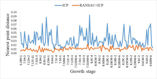
Figure 15.
Comparison of the errors of the two algorithms.
Since the shape of soybeans varies at different growth periods, the numbers of point clouds acquired were also different. In comparing the runtime, the analysis was based on the number of point clouds. In addition, the shape of the soybean canopy point cloud was extremely irregular, so it was normal for the matching time to be long. From Table 1, the ICP algorithm time consumption satisfied a positive linear relationship with the size of the input point cloud. Compared with the registration time of the traditional ICP algorithm, the time required to perform ICP algorithm registration after RANSAC coarse alignment was shorter, and the average registration times for the three ranges of point clouds were reduced by 19.53 s, 44.62 s and 59.96 s. In Figure 15, the horizontal coordinates indicate the numbers of soybean plants, and the vertical coordinates represent the distance to the nearest point. The matching error of the RANSAC + ICP algorithm was between 0.0023 and 0.0230, with an average error of 0.0109, and the error of the traditional ICP algorithm was between 0.0101 and 0.0933, with an average error of 0.0323. The matching accuracy of the former was significantly higher than that of the latter, and the average error of the RANSAC + ICP algorithm was 0.0214 smaller than that of the traditional ICP algorithm. Therefore, the RANSAC + ICP algorithm proposed in this study was suitable for multi-perspective 3D reconstruction of soybean canopy in complex environments with low requirements for real-time performance. Compared with the traditional ICP algorithm, the algorithm was more robust and tolerant to the noise and outliers in the point cloud, and the overall registration results of the canopy point cloud were not easily affected by the noise. Moreover, the generated 3D point cloud of soybean plants had a better visual structure for the subsequent calculation of phenotypic traits for soybean plant.
6. Calculation of Phenotypic Traits
6.1. Calculation of Plant Height
Plant height is an important agronomic trait of soybean that is of great significance to breeding and soybean yield. It was defined herein as the distance from the root neck of the plant to the top.
For effectively selecting the edge points of the whole point cloud, the alpha-shapes algorithm was chosen in this paper. This is a simple and effective fast algorithm for extracting boundary points, which can be used to extract edges from a number of disordered point sets [30]. Supposing that the alpha shape of a point set was a polygon, which was determined by the point set and the radius parameter , for plane point clouds of any arbitrary shape, a circle of radius was rolled around it. If the radius of the rolling circle was small enough, each point in the point cloud was a boundary point. If it was appropriately increased to a certain extent, it rolled only on the boundary points, and the rolling trajectory was the point cloud boundary.
Specific steps were as follows:
- For any point , the radius of the rolling circle was , and all points within a distance of from the point were searched in the point cloud and recorded as the point set .
- Arbitrary points in were selected, and the coordinates of the center of the circle from the coordinates of these two points and were calculated. The principle is shown in Figure 16.
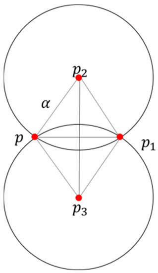 Figure 16. Alpha-shapes calculation schematic.
and were the coordinates of the center of the circle in the two cases of and ; the radius was . The equation for calculating the coordinates was Equation (18):
where
- After removing points from the set of points, the distances from the remaining points to points or were calculated. If the distance from all points to or was greater than , the point was a boundary point.
- If the distance from the remaining points to or was not all greater than , all points in the set of points were traversed and rotated as points. If there was a point satisfying the conditions 2 and 3, the point was a boundary point, the judgment of the point was terminated and the next point was judged. If no point like existed among all the nearest neighboring points in the point set , this indicated that point was a nonboundary point. The effect of the final edge detection in the four growth stages was shown in Figure 17.
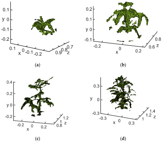 Figure 17. Edge extraction results: (a) flowering stage; (b) podding stage; (c) filling stage; (d) mature stage.
The point cloud processed by the above algorithm resulted in a clear outline of the soybean canopy. When selecting the highest point and the lowest point, invalid points were well avoided, so that the calculation result was close to the real value. The coordinates of the highest point extracted at the flowering stage were (−0.05422, 0.785, −0.03832), and the lowest point was (−0.05414, 0.77, −0.1451). The highest point extracted at the podding stage was (−0.01342, 0.6912, 0.2244), and the lowest point was (−0.01026, 0.713, −0.1249). The highest point extracted at the filling stage was (0.108, 1.121, 0.3506), and the lowest point was (0.04255, 1.15, −0.2293). The highest point extracted at the mature stage was (−0.1008, 1.188, 0.4104), and the lowest point was (−0.09018, 1.043, −0.2523).
The method for acquiring plant height of the soybean canopy was to calculate the spatial distance between the highest and lowest points of the canopy (Figure 18). The calculation method is shown in Equation (19):
where is the highest point and is the lowest point.
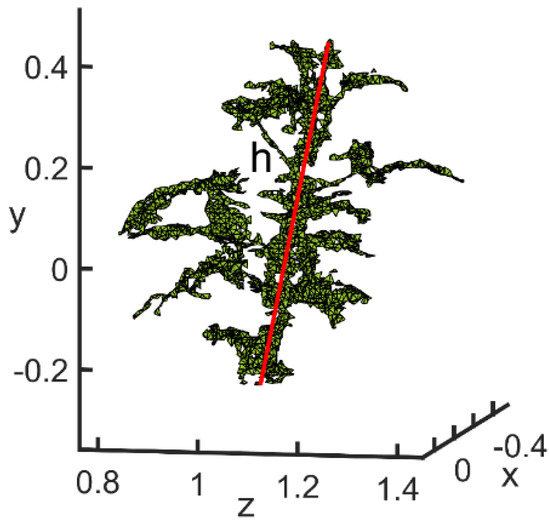
Figure 18.
Plant height calculation diagram.
By the above method, the results for the four growth stages of plant height were 10.78 cm, 35.00 cm, 58.43 cm and 67.85 cm, respectively. The results of the actual measurements were 111.5 cm, 36.8 cm, 60 cm and 69 cm, respectively. Their absolute deviations were 0.72 cm, 1.8 cm, 1.57 cm and 1.15 cm, respectively. The average deviation rates were 6.3%, 4.9%, 3% and 1.7%. Therefore, the 3D structural morphology of the soybean canopy obtained by the above reconstruction method was applied to calculate the plant height of soybean plants with accuracies of 93.7%, 95.1%, 97.4% and 98.3% for different growth periods. This showed that the 3D structural morphology of the soybean canopy obtained by this reconstruction method differed less from the real soybean plant. The plant height deviations of the obtained samples were within the allowable range, which verified the validity of the 3D reconstruction method for soybean canopy.
6.2. Calculation of Leafstalk Angle
Soybean leafstalk angle is an important phenotypic trait that directly affects canopy structure and thus has an important impact on soybean yield. It is important to improve the yield of soybean by improving the plant shape. The leafstalk angle was defined herein as the inclination between the midrib and the stem of the leaf, which consists of branch points and vertices. Take any petiole as an example: the vertex was the intersection of the petiole and the main stem, and the branch point was the end of petiole or the end of main stem. Because soybean plants have an irregular shape, and the branches and leaves block each other, it is difficult to calculate leafstalk angle using traditional 2D images.
Compared with traditional 2D images, a 3D structure of a soybean canopy can provide comprehensive plant phenotype information more conveniently. This allowed us to find the best viewpoint for observing a particular leafstalk angle without the limitation of the field of view. If the points are selected manually within the 3D morphological structure, the spatial influence may lead to deviations in the selection of points. In this paper, in order to calculate the leafstalk angle more accurately, we mapped the 3D point cloud structure of the observation location to the 2D plane after selecting the best observation angle using the orthogonal side projection method [31].
Normal axonometric projection is a projection method in which a three-dimensional structural shape is rotated around the -axis by an angle of , then rotated by an angle of around the -axis and finally projected to the plane . The projection method used was the parallel projection method. The steps of the normal axonometric projection in three-dimensional space were as follows:
- The diagram was rotated by the angle around the -axis, rotated by the angle around the -axis, and then projected to the plane (y = 0). The transformation matrix was . The three matrices were multiplied together to obtain the orthometric projection transformation matrix .
Any given and was transformed into the matrix, the matrix was used to transform the 3D structure to obtain a parallel projection of the 3D point cloud. The matrix composed of the coordinates of each point of the 3D soybean canopy is expressed by Equation (24):
- 2.
- The result of multiplying the vertices with was the coordinates of the transformed vertices. These coordinates were then projected to the surface to obtain a reconstructed orthoaxial side view of the 3D soybean canopy point cloud. Since was a matrix and was an matrix, the two matrices could not be multiplied directly. To make the transformation possible, we used chi-square coordinates, i.e., added a coordinate component to each vertex of the stereogram so that became as follows:
- 3.
- The matrix was used to transform to obtain the projected coordinates of each point of the 3D soybean canopy on the specified plane. In this study, the values of and were adaptive, ranging from 0 to 180°. The projection effect is shown in Figure 19.
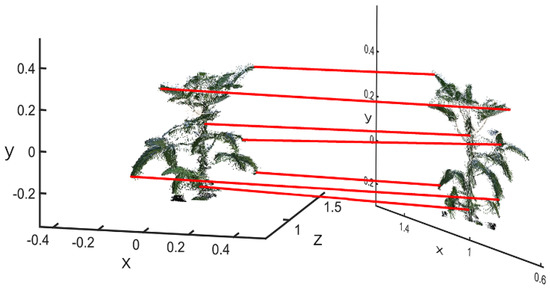 Figure 19. Projection of point cloud.
The projection of point cloud maintained the characteristics of the canopy, and the angle of the peduncle was observed clearly. To distinguish the vertex and branch points of the leafstalk angle, the point cloud of the canopy was projected on a 2D plane after selecting the best viewpoint for observing the leafstalk angle. The color of the point cloud of the canopy part was set to black, and that of the rest to white, by using binarization. Thus, the pixel value of the canopy was 0, while the pixel value of the background was 1. The steps for judging branch points and vertices were as follows [32]:
- A 8-neighborhood template centered on the test point was created and detected point by point according to the projected 3D canopy.
- At each test point, detection was performed point by point according to the detection template as in Figure 20. The feature points detected in this paper were the branch points and vertices of the soybean canopy stalks.
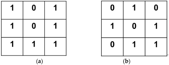 Figure 20. Test results: (a) branch point; (b) vertex point.
When the center point of the template was 0, it meant that this point was valid and could participate in the detection. To eliminate adjacent points and spurious branch points, the value of was calculated by Equation (26):
where was the pixel value and was the value of the center of the template.
- 3.
- If or , the point was a vertex. If , the point was a branch point.
The vertex on the main stem detected by the above method was connected with any branch point above it to form a line segment ; the branch point on the leafstalk was connected to form a line segment ; and the line segment was the edge opposite to the vertex , that is, the line segment connecting the branch points and . Triangle was constructed with vertices at . According to the 3D point cloud information on the soybean plants, the 3D spatial coordinate information of the corresponding points , , and was obtained, and the leafstalk angle was calculated by Equation (27):
where was the angle of the leafstalk and , and are the lengths of the three sides of the triangle.
A diagram of the leafstalk angle is shown in Figure 21. From the top of the soybean canopy, three leafstalk angles were calculated for the flowering and podding stages, and five were calculated at the filling stage and mature stage. Through the calculation of the above method, the calculation results of the leafstalk angles at the flowering stage were 29.8349°, 90.9043° and 47.2386°. The three leafstalk angles at the podding stage were 42.8972°, 37.6307° and 85.0950°. The five leafstalk angles at the filling stage were 52.0119°, 68.0138°, 57.2703°, 53.1517° and 66.9444°. The five leafstalk angles at mature stage were calculated as 65.8847°, 46.0832°, 61.3087°, 62.2047° and 81.5838°. The measured values for the three corners of the flowering stage were 33.1°, 92.2° and 50.4°; those for the podding stages were 44°, 35.8° and 84.6°; those for the filling stage were 56.7°, 69.3°, 55.9°, 56.4° and 67.8°; and those for the mature stage were 63.1, 50.3, 60.9, 60.3, 84.2°. The average deviations calculated for the four growth stageswere 2.5741°, 1.1428°, 2.2898° and 2.3862°, respectively. The accuracy rates for leafstalk angles based on 3D reconstruction were 95.6, 97.9, 96.3, 96.3%, respectively, and the average deviation rates were 4.4%, 2.1%, 3.7% and 3.7%, respectively.
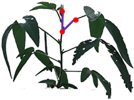
Figure 21.
Diagram for calculating the angle of the leafstalk.
The deviations of the obtained sample leafstalk angles were within the permissible range, which verified that the reconstruction method for the 3D structural morphology of the soybean canopy obtained in this study had some scientific validity and provided the basic conditions for the calculation of leafstalk angle. Meanwhile, from the above calculation results, the average accuracy of the leafstalk angle was above 95%, which verified the accuracy of the 3D reconstruction.
6.3. Calculation of Canopy Width
Canopy width is an important trait in the soybean phenotype. The traditional method of measuring crown width is to measure the length of the canopy in the east–west and north–south directions with a ruler, so as to obtain the crown width of a single soybean plant. Although this method is accurate, it is labor-, cost- and time-consuming. Because of the low resolution and other aspects of the plant canopy image data obtained by satellite remote sensing images, only a large area of canopy can be extracted, and a single plant canopy cannot be effectively extracted. In this study, depth cameras was used to obtain and reconstruct the 3D structure of the soybean canopy, and the 3D reconstruction technology was used to calculate the soybean canopy width nondestructively, quickly, and accurately, which can effectively overcome the aforementioned problems.
According to agronomic requirements, the vertical distance between the farthest lateral point clouds of the canopy projected to the ground was defined as the maximum length of the canopy, and the corresponding longitudinal distance was defined as the maximum width of the canopy. The average of the maximum length of the canopy and the maximum width of the canopy was the crown width. On the basis of the method proposed in Section 4.1, accurate canopy edge points were extracted. Since the coordinate system of the Kinect sensor was different from the Cartesian coordinate system, the maximum axis was the difference between the maximum and minimum values on the axis , and the minimum axis was the difference between the maximum and minimum values on the axis . The average of the maximum canopy widths in the horizontal, vertical and two directions of the soybean canopy were used to represent the canopy width size in this experiment [33]. A schematic diagram of canopy width calculation is shown in Figure 22, and its calculation was as follows in Equations (28)–(30):
where and represent the maximum canopy widths of the soybean canopy in the east–west and north–south directions, respectively.
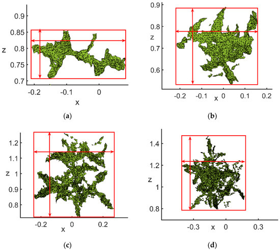
Figure 22.
Schematic of calculation of the canopy width: (a) flowering stage; (b) podding stage; (c) filling stage; (d) mature stage.
Through the calculation of the above method, the calculated values of the maximum axes in the four growth stageswere 0.2180 m, 0.5144 m, 0.5789 m and 0.6450 m, respectively; those of the minimum axes were 0.1062 m, 0.3852 m, 0.5116 m and 0.5486 m, respectively; and those of the crown widths were 0.1621 m, 0.4498 m, 0.5453 m and 0.5968 m, respectively. However, the measured values of the maximum axes were 0.2001 m, 0.509 m, 0.61 m and 0.59 m, respectively; those of the minimum axes were 0.1025 m, 0.49 m, 0.47 m and 0.59 m, respectively; and those of the crown widths were 0.1513 m, 0.4995 m, 0.54 m and 0.59 m, respectively. Therefore, the calculation deviations were 0.0108 m, 0.0497 m, 0.0053 m and 0.0068 m, respectively. It followed that using the reconstructed 3D structural morphology of the soybean canopy to calculate the canopy width, the accuracy rates were 92.9%, 90.1%, 99% and 98.8%, respectively, and the average deviation rates were 7.1%, 9.9%, 1.0% and 1.2%, respectively. Above all, 3D structural morphology reconstructed by the above method had a high degree of reduction.
6.4. Analysis of the Calculation Results of Phenotypic Traits
To further evaluate the effect of the 3D reconstruction, two algorithms were used to study two varieties (Heihe 49 and Suinong 26) at the flowering, podding, filling and mature stages. To accurately find the corresponding measured data for the height, the leafstalk angle, and canopy width, 30 sets of data per plant were selected, and 135 sets of crown width data were used, including single plants and multiple plants.
From the above collected data, scatter plots of calculated data on different phenotypes and actual measured data were fitted to calculate a linear regression equation. The calculated fitting diagrams of different phenotypic traits are shown in Figure 23, Figure 24 and Figure 25.
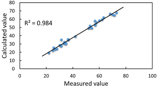
Figure 23.
Linear relationship between calculated and measured values of plant height.
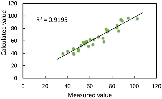
Figure 24.
Linear relationship between calculated and measured values of leafstalk angle.
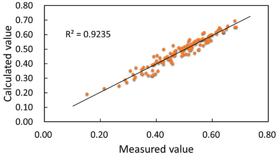
Figure 25.
Linear relationship between calculated and measured values of canopy width.
Figure 23 shows that the coefficient of determination between the calculated and measured values of plant height was 0.984, and the correlation coefficient was 0.9920. These coefficients directly indicated that the plant heights calculated based on the reconstructed 3D soybean canopy were closely related to the measured values. The measured plant height values for the four growth stages, flowering, podding, filling and mature, were in the ranges of 20–25 cm, 25.6–62.2 cm, 53–71.5 cm and 52–73 cm, respectively, and the mean values were 25.44 cm, 37.97 cm, 48.08 cm and 46.04 cm, respectively. The calculated plant height values for the four growth stages were in the ranges of 19.34–23.49 cm, 24.16–59.68 cm, 49.35–66.48 cm and 49.16–67.85 cm, and the mean values were 22.45 cm, 35.57 cm, 45.90 cm and 44.15 cm, respectively. The deviations were 2.99 cm, 2.4 cm, 2.18 cm and 1.89 cm, respectively. The deviations ranged from 0.14 to 6.72 cm, with average and median deviations of 2.84 cm each. The overall deviation distribution for the calculations was relatively dense. From these data, plant height grew faster at the pod stage, which was a critical stage of soybean growth and directly affected soybean yield; plant height peaked at the filling stage, when pods grew vigorously, and plant height decreased slightly from the filling stage to the mature stage. In this paper, we used the reconstructed results for the calculation of plant height, based on the manually measured values. The method in Section 4.1 obtained plant height values more accurately with less deviation, and the reconstruction was more satisfactory, with better accuracy and robustness in calculating the plant height.
As can be seen in Figure 24, the coefficient of determination between the calculated and measured values of leafstalk angle was 0.9195, and the correlation coefficient was 0.9589, which indicated that the method for leafstalk angle calculation based on the 3D reconstructed soybean canopy was scientific and adaptable. The measured values of leafstalk angles for the four growth stages, flowering, podding, filling and mature, were in the ranges of 56.1–87.7°, 35.8–94.5°, 49.7–103.0° and 45.3–89.2°, respectively. The average measured values were 63.63°, 67.93°, 61.30° and 66.88°, respectively. The calculated values of the leafstalk angle were in the ranges of 52.65–94.8°, 39.7–97.2°, 43.82–95.84°, 39.07–92.37°, respectively. The average calculated values were 64.46°, 65.76°, 59.44° and 66.66°, respectively. The deviation range of the overall leafstalk angle was from 0.2023 to 13.6471°; the average deviation was 4.0866°. From the above data, soybeans had overall good growth during the experimental process, and their overall canopy spreading was reasonable. When arriving at the filling stage, the whole soybean plant leafstalk angle reached the peak of growth, with the complete growth and development of pods. The overall canopy of the leafstalk angle showed a shrinking state at the mature stage due to external environmental light factors and internal nutrient distribution. Leafstalk angle was the core of canopy morphology, which directly affected the canopy structure and thus the yield. In addition, from the results of the deviation between the calculated and measured values, the method of calculating the plant leafstalk angle based on the 3D soybean canopy reconstruction was able to calculate the plant leafstalk angle more accurately within a tolerable range of deviation. The main reason for the deviation was the limitations imposed by the minimum recognition accuracy of the hardware and the human deviation in the traditional manual measurement.
The coefficient of determination between the calculated and measured values of crown width 0.9235, and the correlation coefficient was 0.9610, as shown in Figure 25. Both coefficients indicated that the morphological structure of the soybean point cloud was more similar to the real one. The measured values of crown width in the four growth stages, flowering, podding, filling and mature, were in the ranges of 0.1513–0.4500 m, 0.3065–0.5655 m, 0.4025–0.6800 m and 0.4150–0.6850 m, respectively, and the mean measured values were 0.3230 m, 0.4075 m, 0.4544 m and 0.4305 m, respectively. The calculated values were in the ranges of 0.1921–0.4363 m, 0.3263–0.6078 m, 0.4543–0.6518 m and 0.4183–0.6854 m, respectively, and the mean calculated values were 0.2940 m, 0.4013 m, 0.4417 m and 0.4234 m, respectively. The deviation range was 0.0001–0.0740 m, with an average deviation of 0.0213 m and a median deviation of 0.0164 m, indicating a dense deviation distribution. From the trend of the above data, the width of the soybean canopy increased sharply and varied greatly from the flowering to the podding stage. Furthermore, the size of canopy width was influenced by the leafstalk angle. The larger the leafstalk angle was, the larger the canopy width was, provided that all leaves were retained. At the filling stage, the soybean canopy was maximally stretched by the leafstalk in order to allow sufficient light for pod growth. At the mature stage, the leafstalk and leaves began to fall off for physiological reasons, resulting in smaller canopy widths. In this paper, we used the reconstructed results for the calculation of crown width, based on the manually measured values. The method in Section 4.2 obtained the size of crown width more accurately with less deviation. The calculated values of canopy width were closer to the actual soybean crown width measurements than values calculated by traditional methods. The method for canopy width in this paper had high accuracy, with good agreement with the manual measurements.
7. Discussion
A 3D reconstruction algorithm of the soybean canopy based on multivision technology is proposed. Phenotypic traits, including plant height, leafstalk angle and crown width, of soybean plants were calculated based on the 3D reconstruction of the soybean canopy at four growth stages. This technology could provide the basis for breeders to perform virtual breeding based on predicted future meteorological conditions [34]. The experimental results were analyzed as follows:
- Preprocessing. Preprocessing operations such as simplification and denoising of point clouds were important factors affecting data processing speed and calculation accuracy [35]. Because the canopy leaves were relatively densely distributed, the point cloud image from a single perspective could not clearly show the 3D structural morphology of the canopy, and there existed a large number of interference factors such as edge noise and background redundancy, which directly affected the feature extraction, registration and semantic processing of point clouds. In order to solve the above problems, this paper adopted conditional filtering and K-neighbor filtering, which effectively preserved the edge and stem detail characteristics in the raw point cloud. This method was suitable for the simplification of soybean canopy point clouds at different growth stages. The appropriate threshold K should be set for the details of the canopy layer to optimize the filtering results and simplify the canopy point cloud slice model of each viewing angle.
- Point cloud registration. Both the RANSAC algorithm and the ICP registration algorithm used in this paper should be improved to obtain the best reconstructed 3D model of the soybean canopy. In this study, the RANSAC algorithm was used to extract the soybean canopy from complex feature points. In addition, the ICP algorithm was used to achieve accurate and efficient registration between 3D point clouds of three perspectives. Robustness was a key indicator of algorithm evaluation. The correlation results showed that the error of the algorithm was between 0.0023 and 0.0230, and the average error was 0.0109. The RANSAC–ICP algorithm in this study satisfied the requirements of 3D reconstruction and phenotypic analysis of soybean plants.
- Calculation of phenotypic traits. In the field of 3D crop reconstruction, a high-precision 3D point cloud, as an important dataset, was the key to successfully extracting crop morphological characteristics. Three-dimensional point clouds can already be obtained by many methods, such as LiDAR, ultrasonic sensors, scanners and digitizers. Compared with these techniques, the proposed 3D reconstruction method is more economical and more efficient and more realistically restores the color and morphological structure of the plant. Therefore, this method can better extract the quantitative characteristic parameters of soybean plants. The correlation results showed that the coefficient of determination between the calculated value of plant height and the measured value was 0.984. The coefficient of determination between the calculated value of leafstalk angle and the measured value was 0.9195. The coefficient of determination between the calculated value of the canopy width and the measured value was 0.9235.
- Experimental environment. Although the experimental results met the requirements for calculating the phenotypic traits of soybean canopy, some aspects still needed considering in order to obtain more accurate horizontal canopy point cloud data under outdoor conditions. The first relates to environmental factors, and in particular weather conditions. Ideal weather conditions include a windless sunny day. Actual environmental conditions, such as windy or rainy days, cannot be controlled but can be avoided. In the second aspect, attention should be paid to ensure that the shooting background during data acquisition avoids complex environments and has reduced environmental redundancy. This would guarantee the reliability of the collected sample data. This study showed that the Kinect sensor, together with the algorithm, could quickly and accurately measure the plant height, leafstalk angle and canopy width of the soybean canopy. From a plant science and breeding perspective, plant height, leafstalk angle and canopy width can be used for soybean genotype screening and optimal breeding.
- Model error analysis. The reasons for the existence of calculation errors were as follows: first, because of the limitation of the accuracy of the shooting equipment, it was impossible to accurately depict the structural form of the crop at a certain distance. Second, the method of manual measurement and data collection was rough, with inevitable accuracy errors and measurement errors, which would affect the accuracy of the final model calculation. To date, most of the research data on crop plant type selection have been obtained by hand [36]. Plant traits extracted based on 3D models can greatly avoid the damage caused by manual measurements. The 3D reconstruction of the model can permanently preserve the plant morphology of specific varieties in a specific environment, which could provide theoretical and data support for the design breeding model combining fraction breeding and phenotypic breeding.
- Application and extension. This paper presents a method for calculating soybean phenotypic traits based on multivisual 3D reconstruction, which was effectively applied in trait detection of potted soybean plants. Its simple operation, fast calculation and accurate results make it extremely easy to be promoted and applied in agricultural breeding, production and management. The method still needs improving in terms of computational efficiency and optimizing of algorithm parameters to accommodate the intricate spatial arrangement and disturbances of different crops under natural field conditions. Furthermore, the method incorporated a streamlined algorithm for point cloud redundancy data to adapt to the data characteristics of field phenotype acquisition devices such as radar sensors, providing technical support for their combination with field locomotives, navigation systems and drones to nondestructively acquire large point cloud data of field crops and accurately reconstruct the 3D structure of single plants and groups. The research could achieve rapid detection of phenotype traits in field crops.
Similarly, food shortages caused by rapid population growth are growing. Increasing crop yields through traditional crop management methods has become a huge challenge for modern agriculture. The key to increasing yields is to combine the extraction of precise crop phenotypes with traditional management. Understanding the precise phenotypes of soybeans, such as plant height, crown width, plant volume, and canopy area, at specific growth stages can help promote optimal management of agriculture, such as optimizing planting density based on plant volume. The combination of crop 3D models and planting density can undoubtedly provide new avenues for optimal management of agriculture. As high-throughput plant phenotypic analysis techniques continue to evolve, it is inevitable that more plant phenotype information will be obtained and integrated to improve crop management.
8. Conclusions
- In this paper, a soybean multisource data acquisition system based on multiple Kinect V2 sensors was designed to collect point cloud data of soybeans in four growth stages. Conditional filtering was used to filter the point cloud files, and then K-nearest Neighbor filtering was used to reduce noise. The final retention rate of valid points was 95.97%. In addition, the traditional ICP algorithm was improved by using the RANSAC algorithm, and then the ICP algorithm was used for accurate registration. The average matching deviation of the RANSAC–ICP algorithm was 0.0214, smaller than that of the traditional ICP algorithm, and its average run time was 41.37 s, less than that of the traditional ICP.
- Soybean canopies’ phenotypic traits were calculated based on 3D reconstruction of the soybean canopy. The alpha-shapes method was used to perform edge extraction of reconstructed point cloud data. The coefficients of determination between the measured and calculated values of soybean plant height, leafstalk angle and canopy width were 0.984, 0.9151 and 0.9235, respectively. The calculation results enabled accurate and rapid calculation of soybean canopy plant parameters.
This method avoided the shortcomings of traditional manual measurements, which were influenced by various factors. The results can provide not only technical support for optimal soybean selection and breeding, growth monitoring and scientific planting, but feasible method for digital and visual simulation and calculation of soybean plants.
Author Contributions
Conceptualization, X.M.; data curation, F.W. and B.W.; investigation, F.W. and M.L.; methodology, F.W. and X.M.; resources, X.M.; writing—original draft, F.W.; writing—review and editing, X.M. All authors have read and agreed to the published version of the manuscript.
Funding
This study was funded jointly by the National Natural Science Foundation of China (funding code: 31601220), the Natural Science Foundation of Heilongjiang Province, China (funding codes: LH2021C062 and LH2020C080) and the Heilongjiang Bayi Agricultural University Support Program for San Heng San Zong, China (funding codes: TDJH202101 and ZRCQC202006).
Institutional Review Board Statement
Not applicable.
Informed Consent Statement
Not applicable.
Data Availability Statement
All data are presented within the article.
Conflicts of Interest
The authors declare that they have no conflict of interest.
References
- Lin, D. Soybean planting technology and control of flower and pod falling in North China. Agric. Dev. Equip. 2022, 1, 199–201. [Google Scholar]
- Li, C. Principal component analysis of yield traits of major soybean cultivars in northern Heilongjiang Province. Mod. Agric. 2020, 12, 4–8. [Google Scholar]
- Yang, Q.; Lin, G.; Lv, H.; Wang, C.; Liao, H. Environmental and genetic regulation of plant height in soybean. BMC Plant Biol. 2021, 21, 63. [Google Scholar] [CrossRef] [PubMed]
- Ikhajiagbe, B.; Ogwu, M.; Lato, N. Growth and yield responses of soybean (Glycine max [L.] Merr.) accessions after exposure to cadmium. J. Vegetos. 2021, 34, 107–118. [Google Scholar] [CrossRef]
- Kong, L.; Wen, Y.; Jiao, X.; Liu, X.; Xu, Z. Interactive regulation of light quality and temperature on cherry tomato growth and photosynthesis. Environ. Exp. Bot. 2021, 182, 104326. [Google Scholar] [CrossRef]
- Petros, W.; Tesfahunegn, G.B.; Berihu, M.; Meinderts, J. Effectiveness of water-saving techniques on growth performance of Mango (Mangifera indica L.) Seedlings in Mihitsab-Azmati Watershed, Rama Area, Northern Ethiopia. Agric. Water Manag. 2021, 243, 106476. [Google Scholar] [CrossRef]
- Pandey, A.K.; Jiang, L.; Moshelion, M.; Gosa, S.C.; Xu, P. Functional physiological phenotyping with functional mapping: A general framework to bridge the phenotype-genotype gap in plant physiology. Iscience 2021, 24, 102846. [Google Scholar] [CrossRef] [PubMed]
- Ma, X.; Wu, Y.; Shen, J.; Duan, L.; Liu, Y. ML-LME: A Plant Growth Situation Analysis was Model Using the Hierarchical Effect of Fractal Dimension. Mathematics 2021, 9, 1322. [Google Scholar] [CrossRef]
- Wang, C.H.; Liu, D.; Rui-Neng, X.U.; Yang, Y.Q.; Liao, H. Mapping of QTLs for leafstalk angle in soybean. Acta Agron. Sin. 2020, 46, 9–19. [Google Scholar]
- Xiong, J.; Yu, D.; Liu, S.; Shu, L.; Liu, Z. A Review of Plant Phenotypic Image Recognition Technology Based on Deep Learning. Electronics 2021, 10, 81. [Google Scholar] [CrossRef]
- Zhao, J.; Wang, X.; Tian, H.; Lu, Y.; Liu, H. A fertilizer discharge detection system based on point cloud data and an efficient volume conversion algorithm. J. Comput. Electron. Agric. 2021, 185, 106131. [Google Scholar] [CrossRef]
- Pasinetti, S.; Hassan, M.M.; Eberhardt, J.; Lancini, M.; Docchio, F.; Sansoni, G. Performance Analysis of the PMD Camboard Picoflexx Time-of-Flight Camera for Markerless Motion Capture Applications. IEEE Trans. Instrum. Meas. 2019, 68, 4456–4471. [Google Scholar] [CrossRef] [Green Version]
- Chang, C.; Zhang, Z.; Gao, N.; Meng, Z. Improved infrared phase measuring reflectometry method for the measurement of discontinuous specular objects. Opt. Lasers Eng. 2020, 134, 106194. [Google Scholar] [CrossRef]
- Hu, C.; Kong, L.; Lv, F. Application of 3D laser scanning technology in engineering field. E3S Web Conf. 2021, 233, 4014. [Google Scholar] [CrossRef]
- Jiang, Q.; Shi, Y.E.; Yan, F.; Zheng, H.; He, B.G. Reconstitution method for tunnel spatiotemporal deformation based on 3D laser scanning technology and corresponding instability warning. Eng. Fail. Anal. 2021, 125, 105391. [Google Scholar] [CrossRef]
- Bi, S.; Yuan, C.; Liu, C.; Cheng, J.; Cai, Y. A Survey of Low-Cost 3D Laser Scanning Technology. Appl. Sci. 2021, 11, 3938. [Google Scholar] [CrossRef]
- Jensen, M.N.; Helles, O.G. Measuring the end-face of silicon boules using mid-infrared laser scanning. CrystEngComm 2021, 23, 4648–4657. [Google Scholar] [CrossRef]
- Majeed, Y.; Zhang, J.; Zhang, X.; Fu, L.; Whiting, M.D. Deep learning based segmentation for automated training of apple trees on trell was wires. Comput. Electron. Agric. 2020, 170, 105277. [Google Scholar] [CrossRef]
- Hai, L.; Shu, L.; Ye, Z. Wheat growth process 3D visualization research based on growth model. In Proceedings of the International Conference on Computer and Computing Technologies in Agriculture, Jilin, China, 12–15 August 2017; Springer: Cham, Switzerland, 2017; Volume 545, pp. 217–231. [Google Scholar]
- Wu, D.; Ye, J.L.; Wang, K.; Geng, Z.; Fu, J.; Liu, L.; Yang, W. Research on 3D reconstruction method of potted rice based on contour projection. J. Agric. Sci. Technol. 2020, 22, 87–95. [Google Scholar]
- Zhu, B.; Liu, F.; Zhu, J.; Guo, Y.; Ma, Y. 3D quantification of plant growth dynamics in a field based on machine vision. Trans. Chin. Soc. Agric. Mach. 2018, 49, 256–262. [Google Scholar]
- Ruchay, A.; Kober, V.; Dorofeev, K.; Kolpakov, V.; Miroshnikov, S. Accurate body measurement of live cattle using three depth cameras and non-rigid 3-D shape recovery. Comput. Electron. Agric. 2020, 179, 105821. [Google Scholar] [CrossRef]
- Alaei, M.; Kokkeler, A.; Boer, P. Vector Modulator-Based Analog Beamforming Using the Least Euclidean Distance Criterion. J. IEEE Access 2021, 9, 65411–65417. [Google Scholar] [CrossRef]
- Cai, Y.; Xu, W.; Zhang, F. ikd-Tree: An Incremental K-D Tree for Robotic Applications. arXiv 2021, arXiv:2102.10808. [Google Scholar]
- Lu, J.; Qian, W.; Li, S.; Cui, R. Enhanced K-Nearest Neighbor for Intelligent Fault Diagnosis of Rotating Machinery. Appl. Sci. 2021, 11, 919. [Google Scholar] [CrossRef]
- Guan, G.; Gu, W. Reconstruction of propeller and complex ship hull surface based on reverse engineering. J. Mar. Sci. Technol. 2019, 27, 498–504. [Google Scholar]
- Tao, H.; Da, F. An automatic point cloud alignment method based on normal vectors. Chin. J. Lasers 2013, 40, 184–189. [Google Scholar]
- Wongkhuenkaew, R.; Auephanwiriyakul, S.; Chaiworawitkul, M.; Theera-Umpon, N. 3D Tooth Model Reconstruction Using Statistical Randomization-Based Particle Swarm Optimization. Appl. Sci. 2021, 11, 363. [Google Scholar] [CrossRef]
- Nguyen, H.; Tan, T.; Wang, Y.; Wang, Z. 3D Shape Reconstruction from Single-shot Speckle Image Using Deep Convolutional Neural Networks. Opt. Lasers Eng. 2021, 143, 106639. [Google Scholar] [CrossRef]
- Liao, Z.; Liu, J.; Shi, G.; Meng, J. Grid Partition Variable Step Alpha Shapes Algorithm. Math. Probl. Eng. 2021, 2021, 5073562. [Google Scholar] [CrossRef]
- Tang, D.; Yan, T. Orthogonal side projection of 3D figures and fading of convex polyhedral. Intell. Comput. Appl. 1994, 1, 23–26. [Google Scholar]
- Zhu, K.; Ma, X.; Guan, H.; Feng, J.; Yu, S. A method of calculating the leafstalk angle of the soybean canopy based on 3D point clouds. Int. J. Remote Sens. 2021, 42, 2463–2484. [Google Scholar] [CrossRef]
- Huang, S.; Wang, H.; Wang, X.; Liang, H.; Pan, W. Effect of ionic rare earth mining on oil tea plant configuration. Environ. Dev. 2019, 31, 224–226. [Google Scholar]
- Ying, L.; Wei, W.; Teng, M.; Sheng, W.; Ze, Y.; Xiao, W.; Chun, Z. Automatic organ-level point cloud segmentation of maize shoots by integrating high-throughput data acquisition and deep learning. Comput. Electron. Agric. 2022, 193, 106702. [Google Scholar]
- Li, R.; Yi, L.; Zhao, W.; Chen, F. Measurement Method of Thermal Protection Layer Thickness of Solid Rocket Motor Based on Laser Point Cloud. J. Solid Rocket. Technol. 2021, 44, 112–117. [Google Scholar]
- Rong, Z.; Kai, S.; Zhuang, Y.; Xue, Y.; Jiang, Y.; Jia, S.; Zhen, H.; Hong, J.; Da, X.; Zhan, Z.; et al. Analysing the phenotype development of soybean plants using low-cost 3d reconstruction. Sci. Rep. 2020, 40, 2352–2357. [Google Scholar]
Publisher’s Note: MDPI stays neutral with regard to jurisdictional claims in published maps and institutional affiliations. |
© 2022 by the authors. Licensee MDPI, Basel, Switzerland. This article is an open access article distributed under the terms and conditions of the Creative Commons Attribution (CC BY) license (https://creativecommons.org/licenses/by/4.0/).