Innovative Living Mulch Management Strategies for Organic Conservation Field Vegetables: Evaluation of Continuous Mowing, Flaming, and Tillage Performances

Abstract

Organic vegetable production is particularly affected by weed pressure and mechanical weeding is the major tactic implemented by growers to keep weeds under economic thresholds. Living mulch (LM) has been shown to provide several environmental services; however, LM management is required to avoid competition between service crops and cash crops. The aim of this trial was to evaluate two innovative LM-based management systems: a system that provided LM growth regulation by means of flaming (LM-FL) and a system where the LM was regularly mowed by an autonomous mower (LM-AM), both compared with a control without LM and based on standard tillage operations (TILL). The three management systems were evaluated in terms of crop production, weed control, and energy consumption on a 2 yr organic crop rotation of cauliflower (Brassica oleracea L. var botrytis) and eggplant (Solanum melongena L.). LM-AM produced an acceptable fresh marketable yield for both vegetable crops. Moreover, the weed dry biomass obtained in LM-AM-managed plots was lower compared to the LM-FL plots and ranged approximately from 200 to 300 kg ha⁻¹. Furthermore, LM-AM management resulted in lower energy consumption (−2330 kWh ha⁻¹ with respect to the TILL system and −7225 kWh ha⁻¹ with respect to the LM-FL system). The results of this trial suggest that autonomous mowers have a great potential to improve LM management and help with implementing sustainable organic vegetable systems.

1. Introduction

1.1. Organic Farming and Non-Chemical Weed Control

Organic farming systems provide a range of ecosystem services with the aim of improving the production process and final product quality [1]. Furthermore, organic farming systems provide a reduction in energy consumption [2] and greenhouse gases (GHG) emissions [3]. However, several studies have highlighted that organic farming system yields are generally lower compared to yields obtained from traditional farming systems [4,5]. In organic farming systems, due to the ban of herbicide use, weed pressure is recognized as the greatest hindrance to crop production [6]. Yield losses mainly occur due to the ability of weeds to compete with the cash crop for resources such as nutrients, light, and water. Despite these dynamics being well known, it is difficult to determine the relationships between yield losses and weed abundance and composition, as many interacting factors must be considered [7]. Moreover, organic farmers generally rely on a range of multiple weed control techniques such as cultural methods, thermal weeding, mechanical removal, or cultivation, all leading to variable results in terms of crop yield and weed control [8]. Inversion tillage (e.g., moldboard plowing) is one of the main weed control strategies in organic farming systems [9]. Its action works mainly through soil burial and uprooting of weed seedlings, agamic propagules, and seeds [10]. It is well known that this type of practice exploits negative effects such as water and organic matter losses, increased CO₂ emissions, nitrate leaching, excessive soil compaction and erosion, and biodiversity reduction [11]. Shallow (~15 cm), non-inversion tillage and no-tillage are thus becoming more common in European organic farming systems [12] to contrast conventional tillage drawbacks. Nevertheless, reduced or no-till practices, when constantly implemented over time, have been shown to promote weed encroachment, especially for perennial weeds [13], which may create a very challenging scenario. On the other hand, diversified crop rotations, including crops with different growing cycles (e.g., winter or summer growing), also entailing the diversification of tillage operations and techniques, may prevent weed species’ adaption to the specific tillage systems through resource competition, allelopathic interference, soil disturbance, and mechanical damage [14,15]. An adequate crop sequence, including also cover crops, grown either in between or within main crop cycles, may affect weed seed-bank composition, reduce weed infestation levels, and prevent difficult weed infestations such as perennials [16].

1.2. Living Mulch Weed Control and Management

Cover crops can be introduced into crop rotations as living mulch (LM), i.e., establishing cover crops in cash crop stands and letting them grow together in an intercropping association at least for one part of the cash crop cycle. Thanks to the continuous soil cover established both in time and space, LMs have shown the potential to protect the soil against erosion; reduce nitrate leaching; increase soil and water quality; enhance microbial, vegetal, and animal biodiversity; and have shown an acceptable weed control effect in vegetable crops [17,18]. LM advantages strictly depend on their management (i.e., species employed, sowing time, seeding rates, tillage operations, weed flora composition, availability of water and nutrients, climatic conditions, and so on), and the magnitude of their benefits is positively correlated with their biomass production [19,20]. On the other hand, excessive growth of the LM can lead to overgrowing the main crop, thus causing competition and, if this occurs at key growing stages of the crop, yield losses. Indeed, carefully planned LM management may improve weed management and environmental benefits and minimize potential negative effects for crop production [21]. In particular, efficient LM management, enabling the LM to deliver ecosystem services to support the main crop growth and avoiding competition between the LM and the main crop, represents a big challenge for this cultural method. Innovative strategies and technologies are needed to increase the economic and agronomic feasibility of LM systems. Among thermal weed control methods, flame weeding can be considered the most widely used in organic farming systems, especially for vegetable production [22,23]. Intense flames are obtained by burning liquefied petroleum gas (LPG) [24]. The most effective use of flaming is to control early emerged weed seedlings [23]. Flaming has also been shown to be more effective on broad-leaved weeds [25]. In field vegetable crops, promising results have been reported by the combination of flaming and mechanical weed control techniques [26]. Mechanical weed control may be fulfilled by numerous devices that generally aim to remove aboveground weed biomass [27]. Mowing is a common mechanical technique for weed control that allows the maintenance of a short weed canopy height and balances water and nutrients between weeds and crops [28]. Different studies have shown that mowing allowed an acceptable weed control effect together with lower energy consumption and GHG emissions [29,30,31]. Despite it representing a valid alternative to chemical herbicides, mechanical weed control is still a challenging field of study for which the scientific literature shows contrasting results [32]. Mechanical weed control efficiency may further increase with the introduction of precise and autonomous machines [33]. For instance, autonomous mowers have been tested in agricultural contexts [29,31,34] showing improved weed control action without a significant increase in energy requirements.

The aim of this trial was to evaluate the suitability and efficiency of three different organic farming management systems. Specifically, tests have been carried out on a 2 yr crop rotation of a fall–winter growing cauliflower (Brassica oleracea L.var botrytis) and spring–summer growing eggplants (Solanum melongena L.) planted on a conventional tillage system (TILL), an LM-based system managed with flaming (LM-FL), and an LM-based system managed with an autonomous mower (LM-AM). The three management systems were evaluated in terms of crop production, weed control effect, and energy consumption.

2. Materials and Methods

2.1. Experimental Design

A two-year trial has been carried out at the Centre for Agri-Environmental Research “Enrico Avanzi” (CIRAA) of the University of Pisa, San Piero a Grado, Pisa, Italy (43°40′ N, 10°20′ E, 0 m a.s.l.) from March 2019 to November 2021. On the studied fields, an organic crop rotation of cauliflower (F1 hybrid ‘Janvel’) and eggplant (F1 hybrid ‘Dalia’) was planted with a plant density of 12,500 plants per hectare (0.8 × 1.0 m). Cauliflowers−eggplants is a typical Mediterranean vegetable crop rotation. Moreover, the plant density of both vegetables was suitable for the random trajectories of operating an autonomous mower provided for the LM-AM plots. The climate is a typical Mediterranean climate, with seasonal peaks of rainfall in spring and fall with a total average annual rainfall of 907 mm and a mean annual temperature of 15 °C. The soil was classified as Typic Xerofluvent, according to the USDA taxonomy, and had a loam sandy texture (81 g 100 g⁻¹ sand, 13 g 100 g⁻¹ silt, 6 g 100 g⁻¹ clay). In the first 30 cm of depth, the soil pH was 6.7, the total N (1.3 mg g⁻¹, Kjeldahl method) and soil organic matter (2.2 g 100 g⁻¹, Walkley–Black method) contents were good, whereas the available P content was low (5 mg kg⁻¹, Olsen method). Cation exchange capacity was 11 meq 100 g⁻¹ and electrical conductivity was 113 μS cm⁻¹. The experimental layout was a completely randomized block design with three replications for a total of 9 experimental plots of 112 m² (5.6 × 20 m). Each experimental plot consisted of a different organic management strategy. Three different management systems were compared: (i) a no-till system based on a permanent living mulch mowed by an autonomous mower (hereafter referred to as LM-AM), (ii) a no-till system based on a permanent living mulch managed with flaming (LM-FL), and (iii) a standard system based on conventional tillage and without living mulch (TILL). The entire experimental field was divided into two parts to achieve a one-year time offset of the crop rotations. The living mulch used for this study consisted of a micro clover (Trifolium repens L. var. Pipolina) and was hand seeded in March 2019 and March 2020 with a seed rate of 10 g m⁻². A Case IH CVX tractor (CNH Industrial, Turin, Italy) powered by a 144.0 kW diesel engine was employed for tillage operations. A Fiat 70–90 tractor (Fiat CNH Industrial, Turin, Italy) powered by a 52.2 kW diesel engine was employed for all the other operations (

Table 1. List of operations carried out during the trial for TILL, LM-FL, and LM-AM plots.

Operation		Number of Operations		Plots
		Year 1 *	Year 2 **	TILL	LM-FL	LM-AM
Seed-bed preparation and cover crop establishment	Tillage 25 cm (combined cultivator)	1	1	✓	✓	✓
	Tillage 15 cm (rotary hoe)	1	1	✓	✓	✓
	Cover crop hand seeding	1	1	-	✓	✓
	rolling (compacting roller)	1	1	-	✓	✓
Weed control treatments	Autonomous mower installation	1	1	-	-	✓
	Weed control (backpack flaming machine)	4	4	-	✓	-
	Weed control (cultivation at 4–5 cm of depth)	4	4	✓	-	-
Crop transplantation and harvest	Vegetable transplantation	2	2	✓	✓	✓
	Cauliflower harvesting	1	1	✓	✓	✓
	Eggplant harvesting	5	5	✓	✓	✓

* Year 1 refers to the crop rotation (cauliflower–eggplant) during 2019 and 2020. ** Year 2 refers to the crop rotation (cauliflower–eggplant) during 2020 and 2021. ✓: the specific operation in column was fulfilled in the treatment plots reported on the rows.

). In February 2019, prior to the living mulch seeding, the whole studied area was tilled (at a depth of 25 cm) with a Mandam top 3 m wide combined cultivator, equipped with curved shanks provided with twist deflectors, couples of concave discs, and a ring roller (Mandam, Gliwice, Poland), and then the seedbed was established by an Alpego Rotozappa FZ rotary harrow 5 m wide (Alpego, Lonigo (VI), Italy), working at a 15 cm depth. The living mulch was left growing until it reached the average canopy height of 15 cm. Subsequently, all the plots grown with the living mulch were mowed in order to bring the average canopy height to 5 cm. On all the experimental plots, irrigation water was supplied during the whole vegetable growing season by means of sprinklers with an inter-space of 7 m. The water volume provided for the cauliflower was approximately 2400 m³ ha⁻¹ for both years, while the eggplants’ water volume was 4900 m³ ha⁻¹ in 2020 and 5100 m³ ha⁻¹ in 2021. The cauliflowers were transplanted on 1 August 2019 and 4 August 2020 using a prototype of a vegetable transplanter developed by Frasconi et al. [35]. The abovementioned machine allows the successful transplantation of vegetable seedlings in both tilled and no-tilled soils. In addition, the machine is able to precisely release solid fertilizers within the furrow by means of a pneumatic spreader APV PS 200 (APV Technische Produkte GmbH ZENTRALE Dallein 15, Hötzelsdorf, Austria) placed on the frame of the machine to boost the vegetable seedlings’ initial growth. Dry blood meal (Orgazot^®, 14-0-0, AGM Fertilizzanti srl, Castelnovo di Sotto (RE), Italy), rock phosphates (Fosfonature 26^®, 0-26-0, TIMAC AGRO Italia spa, Milano (MI), Italy), and potassium sulfate (KALISOP^®, K+S Minerals and Agriculture GmbH, Kassel, Germany) were applied, respectively, at 747, 150, and 234 kg ha⁻¹ on cauliflower, and at 700, 250, and 300 kg ha⁻¹ on eggplants. Eggplants were transplanted with the same machine on 5 May 2020 and 3 May 2021 after the cauliflowers. On each experimental plot and for each crop rotation, 150 plants were transplanted on six rows (25 plants per row). For the TILL plots, additional tillage at a 15 cm depth was provided with the Alpego Rotozappa FZ rotary harrow prior to the vegetable transplantation (both cauliflowers and eggplants).

After transplantation, three Husqvarna Automower 310 (Husqvarna, Stockholm, Sweden) were installed in the LM-AM plots (one per plot) and set to work three days per week. The autonomous mower’s size (length 63 cm × width 51 cm × height 25 cm, with a cutting width of 22 cm) allowed it to move between the plants. The Husqvarna Automower 310’s working capacity is 1000 (±20%) m² d⁻¹ (charging time included and with a random mowing pattern). Thus, the mowing time was set to 4 h per day (charging time excluded) to manage the trial plots of 112 m². To avoid eventual damages to the transplanted vegetables, a customized plastic cylinder was mounted at the base of each plant in the LM-AM plots and fixed to the ground (Figure S1 in Supplementary Material). The cover crop established in the LM-FL plots was managed by means of two flaming treatments per crop rotation (Table 1). Flaming was applied manually with a prototype of a backpack flaming machine developed at the University of Pisa [36]. The operative characteristics of the backpack flaming machine are reported in Section 2.4. On TILL plots, weed control was achieved by means of four shallow tillage operations (Table 1). A 1.5 m wide precision hoeing machine, equipped with a central goose-foot sweep and two side ‘L’-shaped sweeps, along with flexible-tine torsion weeders for intra-row selective weed control, was used at a very reduced soil depth (4–5 cm) [37]. No other field operations were implemented before harvest in all the crops.

2.2. Crop, Living Mulch and Weed Assessments

The manual harvesting of vegetables was fulfilled on 4 December 2019 and 10 December 2020 for the cauliflower. For the eggplant, multiple harvests were performed on 22 July, 30 July, 13 August, 31 August, and 20 October 2020 and on 13 July, 29 July, 29 August, 15 September, and 13 October 2021. Vegetable crop biomass production was assessed at harvest time (in correspondence with the last harvest for eggplants) by sampling the aboveground biomass of each crop on 10 plants of the two central rows. Plant samples collected in each sampling area were processed separately. Crop biomass was subdivided into fresh marketable products (i.e., corymbs for cauliflower and fruits for eggplants) and the total plant weights that were fresh-weighed separately. From each of the three total plant samples collected in each plot, a representative subsample of each component (marketable products and plant aboveground biomass) was fresh-weighed and oven-dried at 60 °C until constant weight. The dry material was then weighed to obtain the dry weight. The LM and weed aboveground biomass were assessed on 0.5 m² (1 m wide × 0.5 m long) areas surrounding the harvested plants. Later, the LM and weed biomass were manually separated in the lab (only for LM-AM and LM-FL plots), oven-dried at 60 °C until constant weight, and the dry weight of their total biomass was measured. Furthermore, during the trial, crop and weed visual soil cover was assessed at the species level for both crops and management systems. Surveys were carried out at two phases: cauliflower-head emergence and final harvest [38] on cauliflower fields, and eggplant blooming and final harvest on eggplant fields. At those phases, weed species were recognized and the soil cover was visually estimated according to the Braun–Blanquet scale, and the values have been re-calculated based on the midpoint percentage mean values indicated by [39].

2.3. Autonomous Mower Working Data

A remote sensing system consisting of two Emlid Reach RTK (Emlid Ltd., Hong Kong China) devices along with two software packages to extract and display the data was used. The custom-built software calculates the area mowed by the autonomous mower over a given period, based on the distance traveled and the cutting width. Furthermore, the custom-built software allows the operator to extract different operational data [40]. In this study, the distance traveled was chosen as an operational parameter, and together with the mowed area data (reported as a percentage of the total area) were recorded every 15 min [40]. Working efficiency was calculated as the ratio of the area mowed (obtained by converting the mowed area percentage to m²) and the area theoretically mowed (obtained by multiplying the distance traveled by the autonomous mower’s working width). Area mowed percentage and distance traveled after 4 h of working were used to calculate the work efficiency. The autonomous mowers’ operational data assessments were carried out in September and November 2019 on cauliflower fields and in June and September 2020 on eggplant fields, for a total of four measurements in vegetable fields. In 2021, four measurements were carried out in fields with no plants (obstacle-free) to evaluate the efficiency reduction.

2.4. Energy Consumption

Primary energy consumption was estimated for the three management systems. To assess the electric energy consumption of the autonomous mowers, a power consumption meter (EL-EPM02HQ; Nedis, MC, ’s-Hertogenbosch, The Netherlands) was installed in each LM-AM plot. According to [24], the backpack flaming machine releases 1.88 kg_LPG h⁻¹ when LPG burners work at a pressure of 2 bar and with a nozzle diameter of 0.9 mm.

The fuel consumption of the tractors was estimated using the following equation (Equation (1)):

$$\mathrm{Ch}=\mathrm{Wm}\times \mathrm{Cs}$$

(1)

where Ch is the hourly consumption of the tractor (kg fuel h⁻¹); Wm is the driving power of the tractor (kW) which was calculated by the ratio of its useful power (Wu) and its estimated global efficiency (η_g), which was different for the combined cultivator (0.6), the rotary harrow (0.7), the transplanter, and the precision hoeing machine (0.8); and Cs is the specific consumption of the tractor (kg fuel kWh⁻¹), which, on average for both the tractors’ diesel engines, is equal to 0.22 kg kWh⁻¹. The primary energy requirement of the autonomous mower was calculated considering the efficiency of the Italian National Electric System equal to 0.546 [41]. To estimate the primary energy consumption of the tractor, a conversion factor of 12.03 kWh kg⁻¹ of fuel [42] was used. To estimate the primary energy consumption of the flaming machine, a conversion factor of 12.78 kWh kg⁻¹ [43] was used.

2.5. CO₂ Emission Estimation

To estimate CO₂ emissions produced by the management systems, the following conversion factors were applied: 0.332 kg of CO₂ emission per kWh generated from the public electricity production in Italy [44], 0.265 kg of CO₂ emission per kWh generated by the diesel fuel [44], and 3.01 kg of CO₂ emission per kWh generated by GPL burning [45]. This CO₂ emissions estimation derives from field operations fulfilled during this trial (it is strictly dependent of the primary energy consumption estimation). Therefore, this estimation does not provide information on CO₂ indirect sources.

2.6. Statistical Analysis

The Shapiro–Wilk test was used to assess data normality and the Breusch–Pagan test was used for homoscedasticity. The statistical software SPSS (IBM Corp, Armonk, NY, USA) was used to analyze cauliflower and eggplant fresh marketable yield and dry biomass, as well as weed and LM dry biomass data. To evaluate changes in cauliflower and eggplants’ fresh marketable yield and plants’ dry biomass over years and treatments, data were processed with a general linear model two-way ANOVA (UNIANOVA). UNIANOVA was also used to perform statistical analysis on eggplant weeds dry biomass and cauliflower LM dry biomass. Cauliflower weeds dry biomass and eggplant LM dry biomass did not respect the normality assumption (p-value < 0.05), and thus were analyzed using a generalized linear model (GENLIN) with a gamma distribution and a log link function. Pairwise comparisons were performed with a Bonferroni’s test and by estimating the 95% confidence interval of the difference between the values.

Equation (2):

$$\mathrm{CI}\left(\mathrm{difference}\right)=\left({\mathrm{x}}_1-{\mathrm{x}}_2\right)\pm 1.96\sqrt{{\left({\mathrm{SEx}}_1\right)}^2+{\left({\mathrm{SEx}}_2\right)}^2}$$

(2)

where x₁ is the mean of the first value, x₂ is the mean of the second value, SEx₁ is the standard error of x₁, and SEx₂ is the standard error of x₂. The resulting confidence interval (CI) of the difference between values should not cross the value 0 in order to accept the null hypothesis that the compared values were different. The autonomous mower’s area mowed percentage was analyzed using the extension package ‘drc’ (dose–response curve) of R [46] with a two-stage meta-analysis dose–response model to estimate the parameters and the effective time values [40]. The non-linear function corresponded to a two-parameter asymptotic regression.

Equation (3):

$$\mathrm{f}\left(\mathrm{x}\right)=\mathrm{d}\left(1-\exp \left(-\frac{\mathrm{x}}{\mathrm{e}}\right)\right)$$

(3)

where parameters d (the upper limit of the function for x going to infinity) and e (the steepness of the increase in the function) were estimated from the model. All the graphs were plotted using the extension package ‘ggplot2′ (Elegant Graphics for Data Analysis New York, NY, USA).

3. Results

Figure S2 in the Supplementary Materials shows the weather conditions during the three experimental years. The winters were warmer than the multiannual values while the summer was warmer only in 2019. The three hottest months in terms of mean maximum temperature were August for the three years, with a mean maximum temperature of 30.8°C (2019), 30.7°C (2020), and 30.4°C (2021). For the three years of the trial, the mean minimum temperatures were higher than their multiannual values except for in January 2019 (0.8 °C). The three experimental years were also characterized by significant amounts of rainfall compared to the multiannual trend. The highest monthly rainfall totals were in November 2019 (279 mm), December 2020 (267 mm), and January 2021 (234 mm). Significant rainfall peaks also occurred in July 2019 and June 2020. The driest months were March 2019, July 2020, and March 2021, with the least amount of rainfall ranging from 1 to 3 mm.

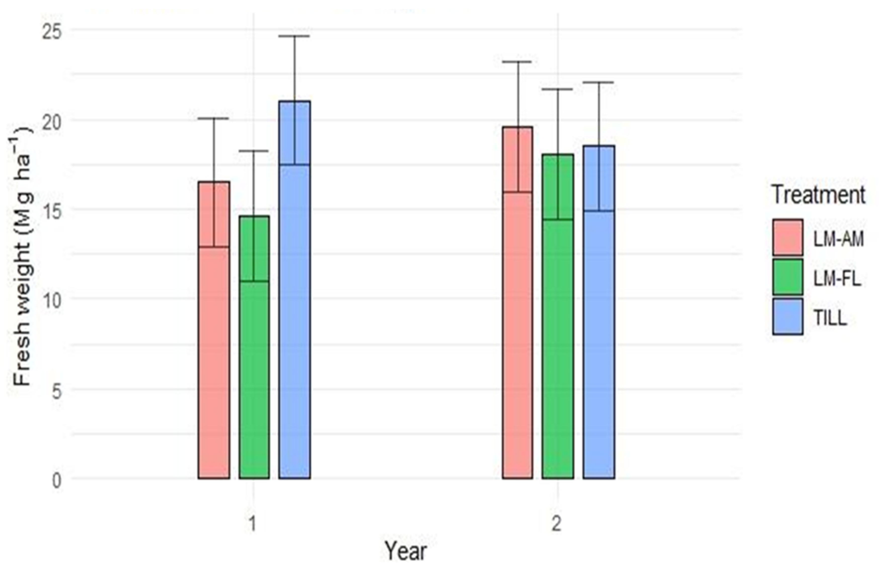
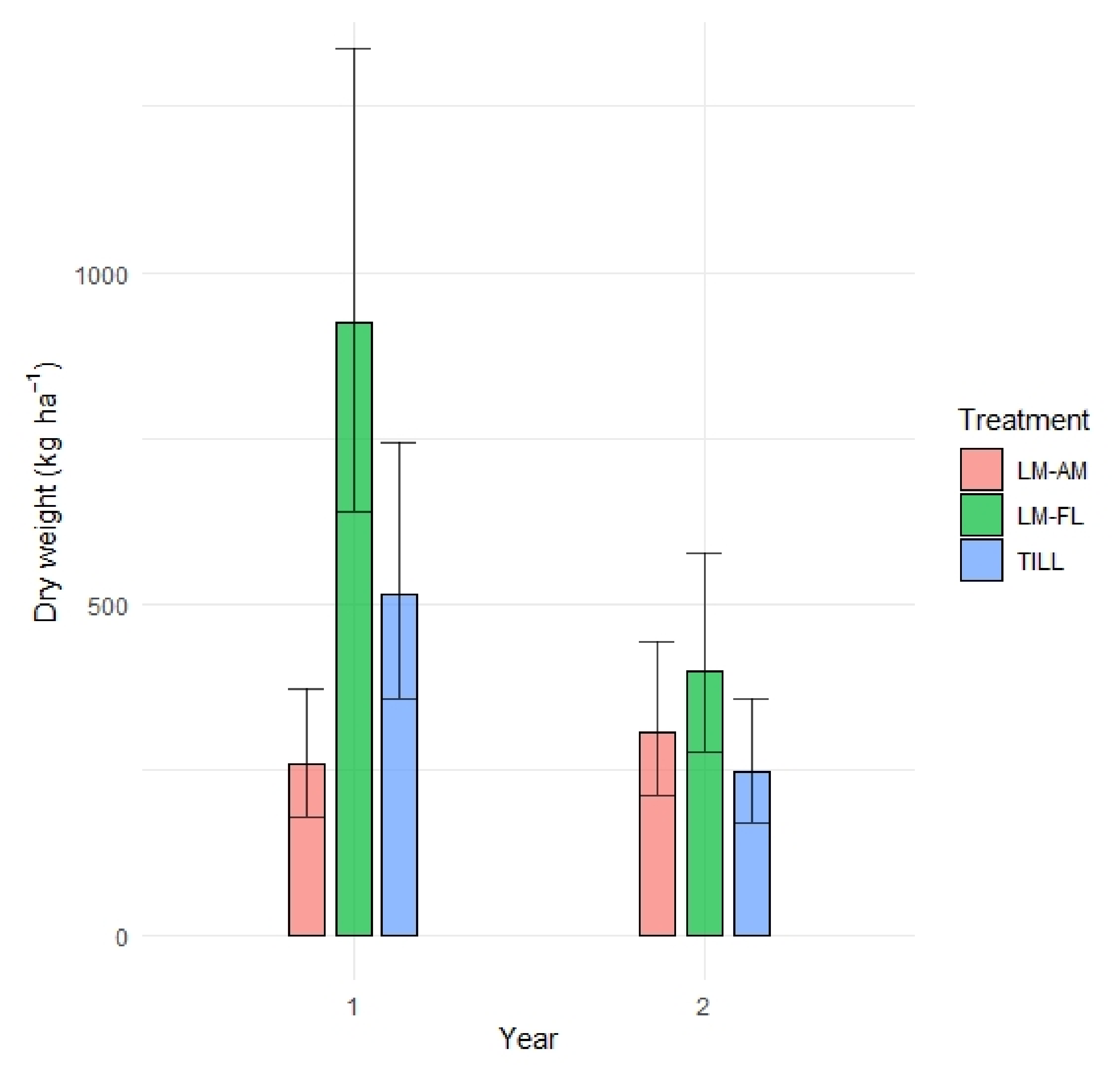
3.1. Cauliflower Data

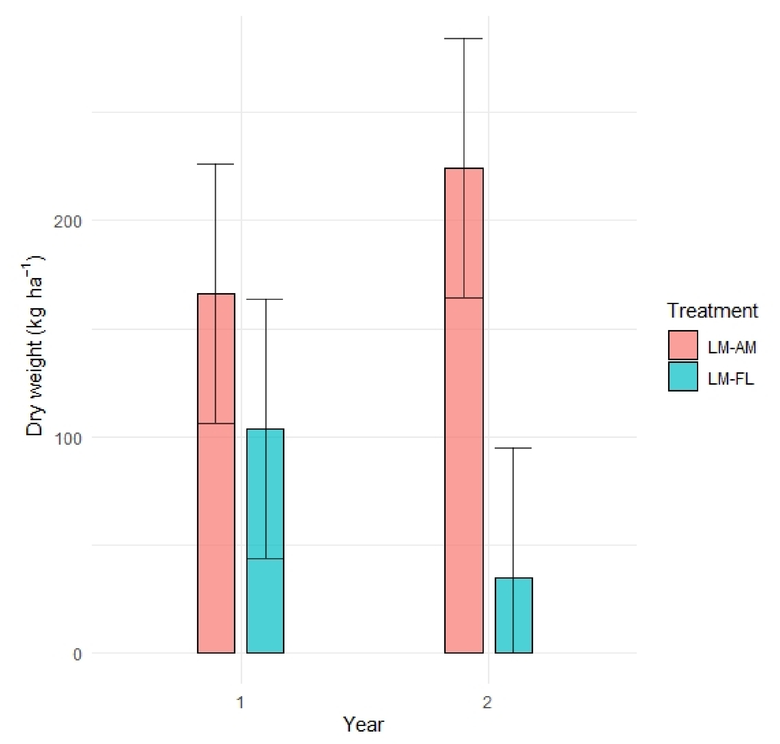
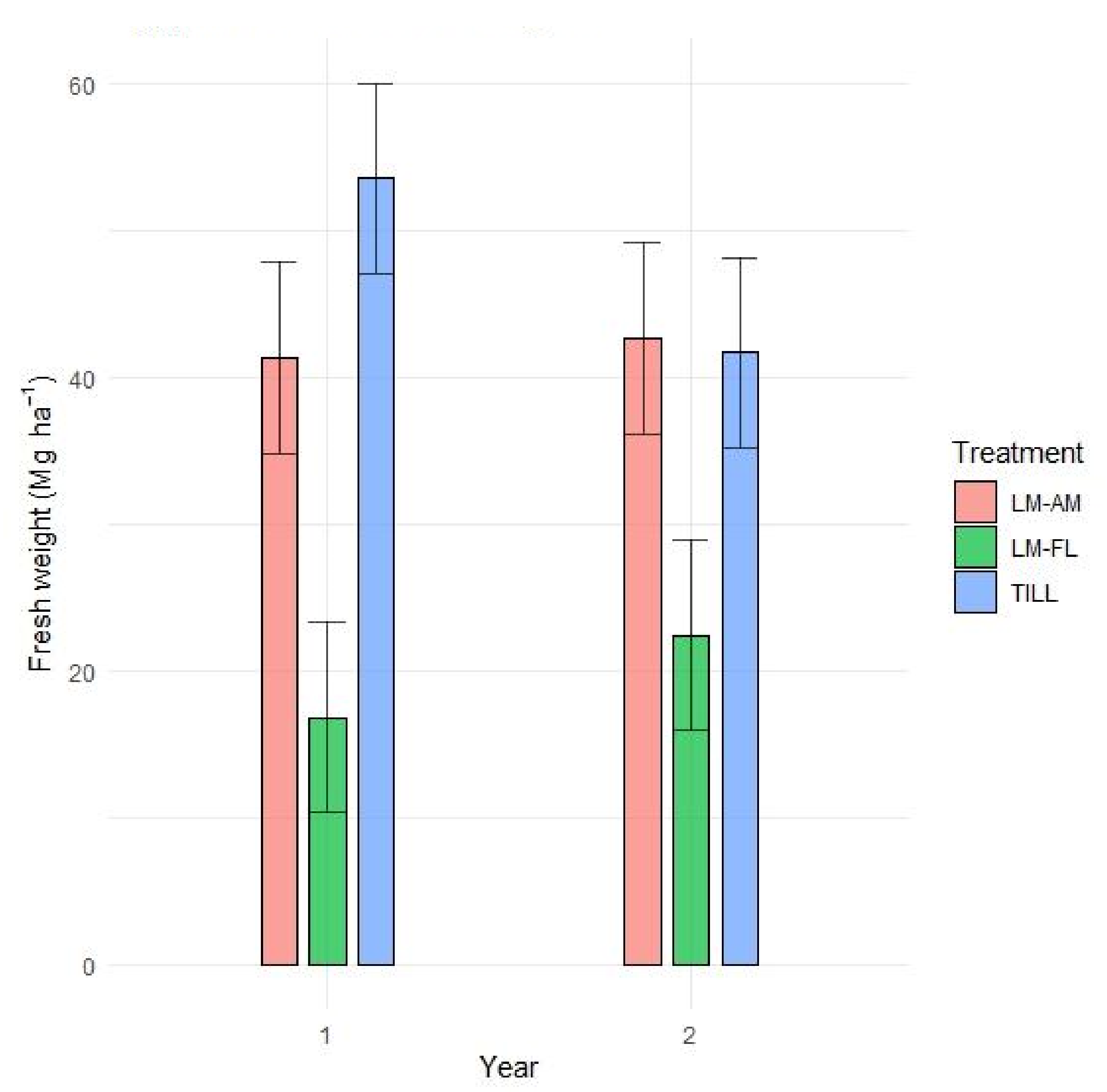
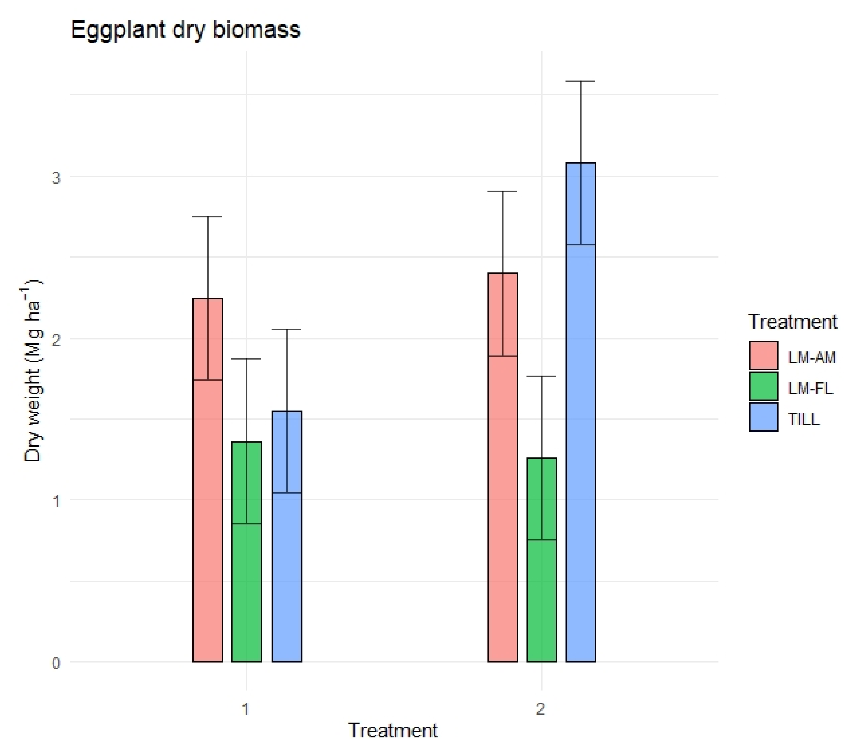
The data of cauliflower fresh marketable yields were normally distributed (p-value = 0.14) and with homogeneous variances (p-value = 0.79). The analysis of variance revealed that the cauliflower fresh marketable yield was not affected by year or treatments (Table S1 in Supplementary Materials). The cauliflower fresh marketable yield ranged from 14.89 to 24.64 Mg ha⁻¹ for the TILL plots, from 11.03 to 21.66 Mg ha⁻¹ for the LM-FL plots, and from 12.89 to 23.17 Mg ha⁻¹ for the LM-AM plots (Figure 1).

The data of cauliflower plants dry weights were normally distributed (p-value = 0.06) and with homogeneous variances (p-value = 0.69). The analysis of variance revealed that the treatment and the interaction between treatment and year significantly affected the cauliflower plants’ dry weight (p-value < 0.001 and < 0.05). Moreover, differences between treatments were found only in the first year (Table S2). In 2019, the plants’ dry weight for the TILL was significantly higher than the LM-FL (p-value < 0.001) and LM-AM (p-value < 0.01). No differences were found in the plants’ dry weights in the second year. Averaged over years, the cauliflower plants’ dry weight was 3.39 Mg ha⁻¹ for the TILL plots, 2.48 Mg ha⁻¹ for the LM-FL plots, and 2.87 Mg ha⁻¹ for the LM-AM plots (Figure 2).

Despite the fact that the data of weed dry weight in cauliflower fields were not normally distributed, homogeneous variances were found (p-value = 0.33). The analysis of variance revealed a significant effect of the year, the treatment, and their interaction (p < 0.01, < 0.001, and < 0.05, respectively) on the total weed dry weight in cauliflower fields (Table S3). The highest weed dry biomass on cauliflower plots was found in the first year in LM-FL plots with an average value of 925.34 (±174.08) kg ha⁻¹. A significant reduction in weed dry biomass was obtained on LM-AM plots in the first year (p-value < 0.01). Weed dry biomass values of LM-AM plots were 258.19 (±48.58) kg ha⁻¹ for the first year and 307.10 (±58.08) kg ha⁻¹ for the second year. The lowest weed dry biomass was measured on TILL plots in the second year with an average of 246.78 (±46.19) kg ha⁻¹ (Figure 3).

Data of LM dry weights in cauliflower fields were normally distributed (p-value = 0.16) and with homogeneous variances (p-value = 0.49). The analysis of variance revealed a significant effect of the treatment and the interaction between year, treatment, and block (p < 0.001, < 0.05, and < 0.01, respectively) on LM dry weights in cauliflower fields (Table S4). The LM dry weight was higher in LM-AM plots than LM-FL during the second year (224.29 kg ha⁻¹). LM-FL plots showed the lower LM dry weights during the trial with only 35.09 kg ha⁻¹. No significant differences were found between treatments during the first year of trial (Figure 4).

3.2. Eggplant Data

The data of eggplant fresh marketable production were normally distributed (p-value = 0.37) and with homogeneous variances (p-value = 0.85). The eggplant fresh marketable production was significantly affected by the treatment and interaction between treatment and year (p-values < 0.001 and < 0.05, respectively) (Table S5). The eggplant fresh marketable yield was the highest in the TILL plots for the first year (53.61 Mg ha⁻¹) and for LM-AM plots in the second year (42.73 Mg ha⁻¹). During both years, no significant differences were found between TILL and LM-AM plots fresh yields (Figure 5). Substantial fresh marketable production differences were found between LM-FL plots and other treatments (p-value < 0.001 for both years). Indeed, the fresh yield production obtained from LM-FL plots was significantly lower compared to other treatment yields for both years (Figure 5).

The data of eggplant dry weights were normally distributed (p-value = 0.42) and with homogeneous variances (p-value = 0.59). The analysis of variance revealed a significant effect of the year, the treatment, and their interaction on eggplant dry weights (p-values < 0.05, < 0.001, and < 0.01, respectively) (Table S6). A pairwise comparison revealed that the eggplant dry biomass obtained from LM-FL plots, ranging from 1.261 to 1.363 Mg ha⁻¹, was significantly lower than the dry biomass obtained from other plots (p-value < 0.001 for both years). No significant differences were found between TILL and LM-AM plots dry biomasses for both years (Figure 6). The higher eggplant dry biomass for the first year was obtained in LM-AM plots (2.245 Mg ha⁻¹), while the second year was higher in the TILL plots (3.080 Mg ha⁻¹).

The data of eggplant weeds dry biomass were normally distributed (p-value = 0.19) and with homogeneous variances (p-value = 0.55). The analysis of variance revealed that the year, the treatment, and their interaction significantly affected the eggplant weeds dry biomass (p < 0.001 for all the factors) (Table S7). The most relevant differences in weed dry biomass were found between LM-AM plots and the other treatments (p-value < 0.001 for both years). LM-AM plots showed the lowest weed dry biomass for both years (208.27 kg ha⁻¹ for the first year and 292.64 kg ha⁻¹ for the second year) (Figure 7). The highest weed dry biomass was obtained during the first year in the LM-FL plots (2254.09 kg ha⁻¹). In the second year, no significant differences were found between the weed dry biomasses obtained from TILL plots during both years and LM-FL plots.

Despite the fact that the data of LM dry weights in eggplant fields were not normally distributed, homogeneous variances were found (p-value = 0.57). The analysis of variance revealed that the LM dry biomass was significantly affected by treatments (p-value < 0.001) (Table S8). The LM dry weights in eggplant fields showed a clear difference based on treatments (Figure 8). The higher value of dry weights was obtained during the second year in LM-FL plots (583.22 kg ha⁻¹) while the lower value was obtained in LM–AM plots (52.38 kg ha⁻¹), also during the second year (Figure 8).

Table 2. Binomial name, botanical family, biological group (BG), life cycle, and average midpoint percentage cover values of the major weed species under three different management systems (LM-AM, LM-FL, TILL) and for the two cash crops (cauliflower and eggplant). Data were pooled over years and repetitions. LM-AM: Living mulch autonomously mowed; LM-FL: living mulch managed with flaming; TILL: conventional tillage.

Species	Botanical Family	BG 1	Life Cycle	Cauliflower			Eggplant
				LM-AM	LM-FL	TILL	LM-AM	LM-FL	TILL
Chenopodium album L.	Chenopodiaceae	T	annual	0.08	0.07	0.13	0.19	0.04	0.16
Amaranthus retroflexus L. *	Amaranthaceae	T	annual	0.02	0.17	0.14	0.04	0.24	0.10
Digitaria sanguinalis (L.) Scop.	Poaceae	T	annual	0.16	0.11	0.07	0.17	0.12	0.10
Echinochloa crus-galli (L.) P. Beauv	Poaceae	T	annual	0.06	0.10	0.13	0.01	0.03	0.09
Cyperus spp. *	Cyperaceae	G	perennial	0.02	0.02	0.11	0.02	0.02	0.04
Cynodon dactylon (L.) Pers.	Poaceae	G	perennial	0.17	0.03	0.06	0.01	0.01	0.19
Lysimachia arvensis (L.) U. Manns and Anderb.	Primulaceae	T	annual	-	-	-	-	0.01	0.01
Schedonorus arundinaceus (Schreb.) Dumort	Poaceae	H	perennial	-	-	-	-	0.01	0.01
Veronica persica Poir *	Plantaginaceae	T	annual	-	0.02	0.02	-	-	-
Paspalum spp. *	Poaceae	G	perennial	0.17	0.05	0.01	0.34	0.12	0.04
Fumaria officinalis L.	Papaveraceae	T	annual	-	0.01	0.01	-	0.03	0.01
Setaria italica subsp. viridis (L.) Thell.	Poaceae	T	annual	0.02	0.15	-	0.09	0.04	-
Verbena officinalis L.	Verbenaceae	H	perennial	0.04	0.01	-	-	-	-
Portulaca oleracea L. s.l.	Portulacaceae	T	annual	-	0.02	0.11	-	0.01	0.03
Poa annua L.	Poaceae	T	annual	0.26	0.05	0.06	0.09	0.01	0.03
Solanum nigrum L.	Solanaceae	T	annual	-	0.04	0.05	-	0.07	-
Rumex spp.	Polygonaceae	H	perennial	-	0.05	0.02	-	0.11	0.02
Stellaria media (L.) Vill.	Caryophyllaceae	T	annual	-	-	0.01	-	-	0.01
Geranium molle L.	Geraniaceae	T	annual	-	-	-	-	-	0.01
Ranunculus repens L.	Ranunculaceae	H	perennial	-	-	0.03	-	-	0.05
Erigeron canadensis L. *	Asteraceae	T	annual	-	-	-	-	0.01	-
Symphyotrichum squamatum (Spreng.) G.L. Nesom *	Asteraceae	T	annual	-	-	-	0.02	0.01	-
Senecio vulgaris L.	Asteraceae	T	annual	-	-	0.03	-	-	0.06
Cardamine hirsuta L.	Brassicaceae	T	annual	-	-	-	-	0.02	0.01
Artemisia vulgaris L.	Asteraceae	H	perennial	-	-	-	0.02	-	-
Hypochaeris radicata L.	Asteraceae	H	perennial	-	-	-	-	-	0.01
Plantago lanceolata L.	Plantaginaceae	H	perennial	-	0.07	-	-	0.06	-
Plantago major L.	Plantaginaceae	H	perennial	-	0.03	0.01	-	0.03	0.01
Subtotals				LM-AM	LM-FL	TILL	LM-AM	LM-FL	TILL
Percentage of therophytes (%)				0.60	0.74	0.76	0.60	0.64	0.62
Percentage of hemicryptophytes (%)				0.04	0.16	0.06	0.02	0.21	0.10
Percentage of geophytes (%)				0.36	0.10	0.18	0.37	0.15	0.27
Percentage of annual (%)				0.60	0.74	0.76	0.60	0.64	0.62
Percentage of perennial (%)				0.40	0.26	0.24	0.39	0.36	0.37

¹ Biological groups: T—therophytes; H—hemicryptophytes; G—geophytes. * Invasive species.

shows the major weeds encountered in the trials and their characteristics. LM-AM, LM-FL, and TILL plots showed a similar percentage of annual therophytes on cauliflower fields (60%, 74%, and 76%, respectively) and on eggplant fields (60%, 64%, and 62%, respectively). A higher hemicryptophytes percentage was found in LM-FL-managed plots (16% in cauliflower fields and 21% in eggplant fields). LM-AM-managed plots showed a higher percentage of geophytes in cauliflower fields (36%) and in eggplant fields (37%). Perennial weed percentages (hemicryptophytes and geophytes) were similar in LM-AM, LM-FL, and TILL plots in cauliflower fields (40%, 26%, and 24%, respectively) and eggplant fields (39%, 36%, and 37%, respectively).

3.3. Autonomous Mower Working Data

The recorded data was well fitted to the asymptotic regression model (lack-of-fit test: p = 1.000). Figure 9 shows the relative working path in a plot with 150 vegetable plants (Figure 9a) and the working path in an obstacle-free plot (Figure 9b), as measured during assessments on 31 July 2020 and 7 June 2021, respectively.

The autonomous mower managed an area of 112 m² consisting of the vegetable plots and a small buffer area surrounding the crops with 150 transplanted vegetables (Figure 9a). In this case, the percentage of area mowed was approximately 26.62% (±5.07%) after one hour, 48.18% (±2.82%) after two hours, 63.26% (±4.92%) after three hours, and 73.93% (±4.95%) after four hours of mowing (Figure 9a). When the autonomous mower managed an area of 112 m², free from transplanted vegetables (Figure 9b), the percentage of area mowed was approximately 66.52% (±1.95%) after one hour, 88.20% (±0.80%) after two hours, 94.79% (±0.22%) after three hours, and 98.57% (±0.42%) after four hours of mowing (Figure 9b).

Table 3. Parameters of the non–linear asymptotic regressions (Equation (3)) and effective times of the autonomous mower estimated from the two-stage meta-analysis dose–response model for an area of 112 m² with obstacles and obstacle-free.

Field	d	e	Effective Time (h)
			ET30	ET60	ET90
obstacles *	108.59 (9.73)	222.42 (29.76)	1.32 (0.18)	3.40 (0.46)	8.54 (1.14)
obstacle-free **	99.43 (0.92)	56.59 (1.79)	0.34 (0.01)	0.86 (0.03)	2.17 (0.07)

* Assessments were carried out while 150 transplanted vegetables were established in the plots. ** Assessments were carried out in plots without vegetables. d: the upper limit of the curve; e: determines the steepness of the increase as time; ET30: the time required to mow 30% of the area; ET60: the time required to mow 60% of the area; ET90: the time required to mow 90% of the area.

shows the non-linear asymptotic regression parameters (Equation (3)) and the effective times estimated from the two-stage meta-analysis dose–response model.

According to the estimation, the autonomous mower was able to manage 90% of the area with transplanted vegetables in 8.54 (±1.14) hours when working in an area of 112 m² and 150 vegetable plants. When working in the same area without transplanted vegetables, 90% of the area was mowed in 2.17 (±0.07) hours. Autonomous mowers working with random trajectories in a field with obstacles show an increase in the time needed of approximately +293.55%. Based on the working data extracted by the custom-built software, the autonomous mower traveled an average of 1953.26 (±213.12) m after four hours of mowing in a 112 m² vegetable field and had an average work efficiency of 0.15 (±0.009). In the field without obstacles, the autonomous mower traveled an average of 2620.66 (±66.65) m after four hours of mowing and had an average work efficiency of 0.18 (±0.005). In this case, the work efficiency of the autonomous mower was evaluated after four hours of working; however, working in a field with no obstacles, 90% of the area mowed was achieved approximately after two hours, which provides a work efficiency of 0.28 (±0.007).

3.4. Primary Energy Consumption and CO₂ Emissions Estimation

Table 4. Estimation of primary energy consumption and CO₂ emission equivalents for the different vegetable management systems during the two years of the trial.

Parameter	Operation	TILL	LM-FL	LM-AM
Primary energy consumption (kWh ha−1)	Seed-bed preparation and CC establishment	1222.79 (±37.16)	770.64 (±20.18)	771.11 (±25.52)
	Weed control treatments	1975.57 (±95.44)	7353.32 (±124.71)	97.47 (±0.40)
	Total	3198.37 (±132.60)	8123.96 (±144.89)	868.58 (±25.92)
CO2 emission equivalents (kg ha−1)	Seed-bed preparation and CC establishment	324.04 (±9.85)	204.22 (±5.35)	204.34 (±6.76)
	Weed control treatments	523.53 (±25.29)	22,133.49 (±375.38)	32.36 (±0.13)
	Total	847.57 (±35.14)	22,337.71 (±380.70)	236.70 (±6.90)

Values were pooled over the blocks and summed over the two years of the trial.

shows the primary energy consumption and CO₂ estimation of the three different management systems studied in this trial. The values shown in Table 4 were pooled over different blocks and summed over the two-year trial. The primary energy estimation highlighted that LM-AM allows a significant reduction in energy consumption (−2330 kWh ha⁻¹ with respect to the TILL system and −7225 kWh ha⁻¹ with respect to the LM-FL system) and CO₂ emissions (−611 kg ha⁻¹ with respect to the TILL system and −22101 kWh ha⁻¹ with respect to the LM-FL system).

On LM-AM plots, seed-bed preparation and CC establishment operations accounted for 88.78% of the primary energy consumption, while the weed control, exploited by the autonomous mower, required 11.22%. Conversely, the LM-FL plots employed 9.49% of the primary energy consumption for seed-bed preparation and CC establishment and 90.51% for weed control. The TILL plots’ primary energy requirements ratio was 38.23% for seed-bed preparation and CC establishment and 61.77% for weed-control treatments. Similar trends were found in CO₂ emissions in TILL- and LM-AM-managed plots; however, in LM-FL-managed plots, seed-bed preparation, and CC establishment were responsible for 0.91% of the CO₂ emissions, and weed control treatments accounted for 99.09% of the CO₂ emissions.

4. Discussion

In this trial, two innovative LM management systems (LM-FL and LM-AM) were tested on a two-year field vegetable crop rotation (cauliflower, eggplants) and compared to a conventionally tilled organic management system (TILL) in Mediterranean conditions.

4.1. Marketable Yields and Crop Dry Biomass Production

Over the two years, cauliflower marketable yields did not show clear differences among the three management systems (Table 2). Moreover, the average marketable yields obtained were in line with values reported in central Italy for organic farms (ranging from 13 to 22 Mg ha⁻¹) [47]. These results are encouraging and suggest that the adoption of LM may increase the sustainability of organic cauliflower crops while maintaining an acceptable production. In eggplant fields, no clear differences emerged between LM-AM and TILL management systems for both years. LM-AM- and TILL-managed eggplants provided acceptable yields ranging from 42.73 to 53.61 Mg ha⁻¹. These production values are similar to eggplant yields obtained by [48]. Conversely, the lowest yield in eggplant fields was observed in LM-FL plots for both years. LM-FL plots showed a significantly higher weed biomass (see the next section), and these results corroborate the idea that weed pressure represents a major hindrance to eggplant production in organic conservation systems [35]. Cauliflower plant dry weights, instead, were significantly higher in TILL-managed plots in the first year compared to LM-AM and LM-FL plots (Figure 2). In the second year, no differences among the three management systems were detected. Several authors reported cash crops’ limited vertical root development due to a shallow soil compaction layer [49]. As in this case, the transitional stage from inversion tillage to conservative management was more susceptible to this phenomenon [50]. The eggplant dry biomass was lower in LM-FL plots during the two years, and no differences were found between LM-AM- and TILL-managed plots. The results of cash crop plant dry biomass highlight the potential of the LM-AM technique. Indeed, the generally marketable yield and plant dry biomass were slightly higher in tilled systems [51] due to the higher mineralization rate of soil organic matter, crop residues, and organic fertilizers [52]. However, in both years and crops, LM managed by AM did not show differences with the tilled systems in terms of fresh marketable yields and crop dry biomass, thus demonstrating that the total biomass production of low-input organic conservative systems can be as high as in the standard organic and integrated systems.

4.2. Weed Control

An adequate weed control strategy has been shown to be a significant yield determinant in cauliflower and eggplant fields [53,54]. Reducing weed competition is a major issue for vegetable crops given their quick cycle, low soil cover capability, reduced plant height, and shallow root systems [17,18]. The three management systems studied in this trial showed different results in terms of weed control effects. In general, the LM-AM management system obtained the lowest weed dry biomass in both years and crops (Figure 3 and Figure 7). Moreover, the weed aboveground dry biomass obtained in LM-AM-managed plots showed similar values between cauliflowers and eggplant fields, ranging approximately from 200 to 300 kg ha⁻¹. These similar weed dry biomass values may be the consequence of the autonomous mower’s continuous cutting action and high overlapping, which produced an intense disturbance action. Interestingly, the trend observed was similar in the two crops, despite their different growing cycles, with weeds that were expected to be more aggressive and competitive in eggplants, due to the huge presence of dormant seeds of harmful summer weed species in the experimental fields, such as Amaranthus retroflexus L., Chenopodium album L., and Echinocloa crus-galli L. P. Beauv. (data not shown) [7,14]. Furthermore, the LM-AM plots resulted in a higher geophytic weed percentage (Table 2), confirming that mowing selects for perennial species and for perennial species with a creeping habitus [30,55]. Despite the fact that creeping habitus and quick soil cover are considered appropriate traits for living mulch species [21], in this case, those species consisted of aggressive weeds such as Paspalum spp. and Cynodon dactylon (L.) Pers. The LM-FL and TILL management systems showed higher weed dry biomass values at harvest time in eggplant fields compared to cauliflower fields (Figure 3 and Figure 7). Furthermore, the highest value was measured in the first year in the LM-FL plots (2254.09 kg ha⁻¹). Several authors reported positive results from flaming for organic weed control in vegetable fields [26] and as a CC termination technique to obtain a dead mulch [35,56]. In this study, flaming was tested as an innovative LM managing technique. However, these results highlight that the tested combination of LM and flaming techniques was not effective in terms of weed control. The weed control effect provided by flaming consists of heat transfer to the aboveground plant biomass [57]. In this case, flaming was used to control both LM and weeds in LM-FL plots; however, due to LM’s higher soil cover, the heat was mainly delivered to the LM and led to its withering. As a consequence of the LM layer fading, weeds quickly developed and filled the free space within the field. The LM-FL plots showed the highest hemicryptophytic weed species percentage. Those species were mainly represented by perennial rosette-forming weeds such as Rumex spp. and Plantago lanceolata L. Those findings confirm that thermal weeding techniques are not effective on these weeds’ typology because of the resources stored in their roots [58]. Moreover, the summer weeds community exerts a higher pressure on eggplants, and this was aggravated by the sprinkler irrigation adopted. In this regard, Lai [59] proposed subirrigation as an irrigation method in no-till vegetable systems to precisely provide water for the vegetables and avoid interference with mechanical or thermal weed control. This would also reduce water availability for summer weeds and consequently slow weed development.

4.3. LM Management System

It is well known that LMs provide numerous ecosystem services and can help design sustainable organic agricultural systems [47,56,60]. However, many authors agree that LM management must be provided along their growing cycle to avoid competition with cash crops [35,60]. Despite LM achieving an acceptable soil cover for all the trials and the fact that it did not outgrow the vegetables, it showed different trends between the two treatments (LM-AM and LM-FL) for cauliflower and eggplants. Averaged over treatments, the aboveground dry biomass achieved by the LM at the harvest of eggplants was higher (+120% on the first year and +145% on the second) than for cauliflower (Figure 4 and Figure 8). The LM biomass produced in cauliflower fields was always higher in LM-AM plots, although significant differences were found only in the second year (Figure 4). Conversely, the LM biomass was higher in LM-FL plots for eggplant fields with clear differences in both years. Eggplants were transplanted in succession to cauliflower and the LM was not reseeded between the two crops. The LM employed for this trial consisted of a microclover. Since microclover is not a Mediterranean ecotype, its performance was probably affected by environmental factors. We argue that the AM management was more intense (three mowing operations per week) compared to the flaming (two flaming treatments during the whole season). The combination of the environmental factors and the management strategy may have compromised LM biomass production, especially in eggplants, which is a summer crop, growing in stressful conditions, prone to drought and thermal stresses. However, the higher LM biomass production in eggplant fields refers to values obtained at the last harvest (20 October 2020 and 13 October 2021). The LM was left undisturbed after the second flaming treatment, and together with the environmental conditions, was able to develop its biomass, which is crucial for exploiting LM ecosystem services [56]. In addition, the two innovative LM management systems proposed in this study were evaluated for their efficiency, primary energy consumption, and CO₂ emissions. The continuous mowing exploited by the AM has been proved to provide for short LM and weed height and small-size clippings [31]. These two conditions have been shown to promote nutrient recycling and favor cash crops for increased water and nutritional availability [30]. The results reported in Table 3 corroborate that AM work efficiency significantly decreased as the obstacle density increased [40]. Path planning has been shown to substantially boost AM work efficiency [61] and could be an option in areas with many obstacles such as vegetable fields. However, despite the low AM efficiency (0.15), LM-AM management obtained the lowest primary energy consumption (868.58 kWh ha⁻¹) compared to LM-FL (8123.96 kWh ha⁻¹) and TILL (3198.37 kWh ha⁻¹). The trend of estimated CO₂ equivalent emissions linked to primary energy consumption was in line with primary energy consumption results. These findings highlight that the use of an AM system is able to increase the sustainability of organic conservation vegetable production, providing significant energy savings [29,34]. Bergtold et al. [62] report that major economic costs for conservation agriculture techniques (especially cover crops) are associated with their management; therefore, increasing the autonomous mower’s precision can bring further economic savings [63]. In contrast, as reported by Antichi et al. [35], controlling weeds by flaming was simply not feasible with the operating machines available, emphasizing the need to develop more effective machinery for LM management and weed control to improve organic conservative systems. The findings of this trial highlight that the LM management by means of autonomous mowers may be employed to further increase the sustainability of organic conservation vegetable production systems.

5. Conclusions

This trial highlights that living mulch managed by autonomous mowers benefits organic vegetable production and provides energy savings compared to flaming and conventional tilling. Indeed, autonomous mowers ensured an acceptable vegetable fresh marketable yield and low weed dry biomass with low energy requirements. The results obtained in this trial suggest that autonomous mowers have a great potential for agricultural purposes, even in challenging scenarios such as organic no-till field vegetables. Further works are needed to improve autonomous mowers’ navigation systems, assess the cost-benefits of this management, and investigate more persistent living mulch species. In this regard, the machines need to be tested in horticultural fields with higher plant densities and with solutions that avoid crop damages. Finally, local ecotype species should be tested to constitute permanent living mulch mixtures and achieve higher ecosystem services through a quicker and more persistent soil cover.

References

1. Arunrat, N.; Sereenonchai, S.; Chaowiwat, W.; Wang, C.; Hatano, R. Carbon, Nitrogen and Water Footprints of Organic Rice and Conventional Rice Production over 4 Years of Cultivation: A Case Study in the Lower North of Thailand. Agronomy 2022, 12, 380. [Google Scholar] [CrossRef]
2. Šarauskis, E.; Masilionytė, L.; Juknevičius, D.; Buragienė, S.; Kriaučiūnienė, Z. Energy use efficiency, GHG emissions, and cost-effectiveness of organic and sustainable fertilization. Energy 2019, 172, 1151–1160. [Google Scholar] [CrossRef]
3. Tzilivakis, J.; Warner, D.J.; May, M.; Lewis, K.A.; Jaggard, K. An assessment of the energy inputs and greenhouse gas emissions in sugar beet (Beta vulgaris) production in the UK. Agric. Syst. 2005, 85, 101–119. [Google Scholar] [CrossRef] [Green Version]
4. Kirchmann, H.; Bergström, L.; Kätterer, T.; Andrén, O.; Andersson, R. Can Organic Crop Production Feed the World? In Organic Crop Production—Ambitions and Limitations; Springer: Berlin/Heidelberg, Germany, 2008; pp. 39–72. [Google Scholar] [CrossRef] [Green Version]
5. Seufert, V.; Ramankutty, N.; Foley, J.A. Comparing the yields of organic and conventional agriculture. Nature 2012, 485, 229–232. [Google Scholar] [CrossRef]
6. Kloen, L.; Daniels, H. Onderzoeksagenda Biologische Landbouw & Voeding 2000–2004; Biologica/Wageningen UR: Utrecht, The Netherlands, 2000. [Google Scholar]
7. Zimdahl, R.L. Influence of Competition on the Plant. In Weed-Crop Competition. A Review; Blackwell Publishing Ltd.: Ames, IA, USA, 2004. [Google Scholar]
8. Peruzzi, A.; Martelloni, L.; Frasconi, C.; Fontanelli, M.; Pirchio, M.; Raffaelli, M. Machines for non-chemical intra-row weed control in narrow and wide-row crops: A review. J. Agric. Eng. 2017, 48, 57–70. [Google Scholar] [CrossRef] [Green Version]
9. Doohan, D.; Wilson, R.; Canales, E.; Parker, J. Investigating the Human Dimension of Weed Management: New Tools of the Trade. Weed Sci. 2010, 58, 503–510. Available online: http://www.jstor.org/stable/40891269 (accessed on 7 February 2022). [CrossRef]
10. Jensen, P. Longevity of seeds of four annual grass and two dicotyledon weed species as related to placement in the soil and straw disposal technique. Weed Res. 2009, 49, 592–601. [Google Scholar] [CrossRef]
11. Morris, D.R.; Gilbert, R.A.; Reicosky, D.C.; Gesch, R.W. Oxidation Potentials of Soil Organic Matter in Histosols under Different Tillage Methods. Soil Sci. Soc. Am. J. 2004, 68, 817–826. [Google Scholar] [CrossRef]
12. Failla, S.; Pirchio, M.; Sportelli, M.; Frasconi, C.; Fontanelli, M.; Raffaelli, M.; Peruzzi, A. Evolution of smart strategies and machines used for conservative management of herbaceous and horticultural crops in the mediterranean basin: A review. Agronomy 2021, 11, 106. [Google Scholar] [CrossRef]
13. Thomas, A.G.; Derksen, D.A.; Blackshaw, R.E.; Van Acker, R.C.; Légère, A.; Watson, P.R.; Turnbull, G.C. A multistudy approach to understanding weed population shifts in medium- to long-term tillage systems. Weed Sci. 2004, 52, 874–880. [Google Scholar] [CrossRef]
14. Graziani, F.; Onofri, A.; Pannacci, E.; Tei, F.; Guiducci, M. Size and composition of weed seedbank in long-term organic and conventional low-input cropping systems. Eur. J. Agron. 2012, 39, 52–61. [Google Scholar] [CrossRef]
15. Murphy, C.E.; Lemerle, D. Continuous cropping systems and weed selection. Euphytica 2006, 148, 61–73. [Google Scholar] [CrossRef]
16. Bohan, D.A.; Powers, S.J.; Champion, G.; Haughton, A.J.; Hawes, C.; Squire, G.; Cussans, J.; Mertens, S.K. Modelling rotations: Can crop sequences explain arable weed seedbank abundance? Weed Res. 2011, 51, 422–432. [Google Scholar] [CrossRef]
17. Campiglia, E.; Mancinelli, R.; Radicetti, E.; Caporali, F. Effect of cover crops and mulches on weed control and nitrogen fertilization in tomato (Lycopersicon esculentum Mill.). Crop Prot. 2010, 29, 354–363. [Google Scholar] [CrossRef]
18. Navarro-Miró, D.; Blanco-Moreno, J.M.; Ciaccia, C.; Chamorro, L.; Testani, E.; Kristensen, H.L.; Hefner, M.; Tamm, K.; Bender, I.; Jakop, M.; et al. Agroecological service crops managed with roller crimper reduce weed density and weed species richness in organic vegetable systems across Europe. Agron. Sustain. Dev. 2019, 39, 1–13. [Google Scholar] [CrossRef]
19. Peachey, R.E.; William, R.A.Y.; Mallory-Smith, C. Effect of No-Till or Conventional Planting and Cover Crops Residues on Weed Emergence in Vegetable Row Crop1. Weed Technol. 2009, 18, 1023–1030. [Google Scholar] [CrossRef]
20. Teasdale, J.R.; Brandsæter, L.O.; Calegari, A.; Neto, F.S. Cover Crops and Weed Management. In Non-Chemical Weed Management: Principles, Concepts and Technology; Upadhyaya, M.K., Blackshaw, R.E., Eds.; CABI: Wallingford, UK, 2007; pp. 49–64. [Google Scholar]
21. Vincent-Caboud, L.; Peigné, J.; Casagrande, M.; Silva, E.M. Overview of Organic Cover Crop-Based No-Tillage Technique in Europe: Farmers’ Practices and Research Challenges. Agriculture 2017, 7, 42. [Google Scholar] [CrossRef] [Green Version]
22. Chehade, L.A.; Fontanelli, M.; Martelloni, L.; Frasconi, C.; Raffaelli, M.; Peruzzi, A. Effects of Flame Weeding on Organic Garlic Production. Horttechnology 2018, 28, 502–508. [Google Scholar] [CrossRef]
23. Tei, F.; Pannacci, E. Weed Management Systems in Vegetables. In Weed Research. Expanding Horizons, 1st ed.; Hatcher, P.E., Froud-Williams, R.J., Eds.; John Wiley & Sons Ltd.: Oxford, UK, 2017; p. 367. [Google Scholar]
24. Raffaelli, M.; Frasconi, C.; Fontanelli, M.; Martelloni, L.; Peruzzi, A. LPG burners for weed control. Appl. Eng. Agric. 2015, 31, 717–731. [Google Scholar] [CrossRef]
25. Martelloni, L.; Fontanelli, M.; Frasconi, C.; Raffaelli, M.; Peruzzi, A. Cross-flaming application for intra-row weed control in maize. Appl. Eng. Agric. 2016, 32, 569–578. [Google Scholar] [CrossRef]
26. Martelloni, L.; Fontanelli, M.; Frasconi, C.; Raffaelli, M.; Pirchio, M.; Peruzzi, A. A combined flamer-cultivator for weed control during the harvesting season of asparagus green spears. Span. J. Agric. Res. 2017, 15, e0203. [Google Scholar] [CrossRef]
27. Bhadra, T.; Paul, S. Weed management in sugar beet: A review. Fundam. Appl. Agric. 2020, 5, 1. [Google Scholar] [CrossRef]
28. Garnier, E.; Navas, M.-L. A trait-based approach to comparative functional plant ecology: Concepts, methods and applications for agroecology. A review. Agron. Sustain. Dev. 2012, 32, 365–399. [Google Scholar] [CrossRef] [Green Version]
29. Magni, S.; Sportelli, M.; Grossi, N.; Volterrani, M.; Minelli, A.; Pirchio, M.; Fontanelli, M.; Frasconi, C.; Gaetani, M.; Martelloni, L.; et al. Autonomous mowing and turf-type bermudagrass as innovations for an environment-friendly floor management of a vineyard in coastal tuscany. Agriculture 2020, 10, 189. [Google Scholar] [CrossRef]
30. MacLaren, C.; Bennett, J.; Dehnen-Schmutz, K. Management practices influence the competitive potential of weed communities and their value to biodiversity in South African vineyards. Weed Res. 2019, 59, 93–106. [Google Scholar] [CrossRef]
31. Sportelli, M.; Frasconi, C.; Fontanelli, M.; Pirchio, M.; Raffaelli, M.; Magni, S.; Caturegli, L.; Volterrani, M.; Mainardi, M.; Peruzzi, A. Autonomous mowing and complete floor cover for weed control in Vineyards. Agronomy 2021, 11, 538. [Google Scholar] [CrossRef]
32. Machleb, J.; Peteinatos, G.G.; Sökefeld, M.; Gerhards, R. Sensor-Based Intrarow Mechanical Weed Control in Sugar Beets with Motorized Finger Weeders. Agronomy 2021, 11, 1517. [Google Scholar] [CrossRef]
33. Slaughter, D.C.; Giles, D.K.; Downey, D. Autonomous robotic weed control systems: A review. Comput. Electron. Agric. 2008, 61, 63–78. [Google Scholar] [CrossRef]
34. Hossain, M.; Takahashi, K.; Komatsuzaki, M. Robotic Lawnmower Saves Labor and Operation Costs in a Pear (Pyrus pyrifolia) Orchard. Jpn. J. Farm Work Res. 2020, 55, 143–153. [Google Scholar] [CrossRef]
35. Antichi, D.; Sbrana, M.; Martelloni, L.; Abou Chehade, L.; Fontanelli, M.; Raffaelli, M.; Mazzoncini, M.; Peruzzi, A.; Frasconi, C. Agronomic performances of organic field vegetables managed with conservation agriculture techniques: A study from central Italy. Agronomy 2019, 9, 810. [Google Scholar] [CrossRef] [Green Version]
36. Raffaelli, M.; Martelloni, L.; Frasconi, C.; Fontanelli, M.; Peruzzi, A. Development of machines for flaming weed control on hard surfaces. Appl. Eng. Agric. 2013, 29, 663–673. [Google Scholar] [CrossRef]
37. Raffaelli, M.; Fontanelli, M.; Frasconi, C.; Sorelli, F.; Ginanni, M.; Peruzzi, A. Physical weed control in processing tomatoes in Central Italy. Renew. Agric. Food Syst. 2011, 26, 95–103. [Google Scholar] [CrossRef]
38. Ciaccia, C.; Kristensen, H.L.; Campanelli, G.; Xie, Y.; Testani, E.; Leteo, F.; Canali, S. Living mulch for weed management in organic vegetable cropping systems under Mediterranean and North European conditions. Renew. Agric. Food Syst. 2017, 32, 248–262. [Google Scholar] [CrossRef]
39. van der Maarel, E. Transformation of cover-abundance values for appropriate numerical treatment—Alternatives to the proposals by Podani. J. Veg. Sci. 2007, 18, 767–770. [Google Scholar] [CrossRef]
40. Sportelli, M.; Pirchio, M.; Fontanelli, M.; Volterrani, M.; Frasconi, C.; Martelloni, L.; Caturegli, L.; Gaetani, M.; Grossi, N.; Magni, S.; et al. Autonomous mowers working in narrow spaces: A possible future application in agriculture? Agronomy 2020, 10, 553. [Google Scholar] [CrossRef] [Green Version]
41. Pirchio, M.; Fontanelli, M.; Labanca, F.; Sportelli, M.; Frasconi, C.; Martelloni, L.; Raffaelli, M.; Peruzzi, A.; Gaetani, M.; Magni, S.; et al. Energetic Aspects of Turfgrass Mowing: Comparison of Different Rotary Mowing Systems. Agriculture 2019, 9, 178. [Google Scholar] [CrossRef] [Green Version]
42. ISPRA—Istituto Superiore per la Protezione e la RicercaAmbientale. Rapporti 280/2018. Available online: https://www.isprambiente.gov.it/files2018/pubblicazioni/rapporti/R_280_18_Emissioni_Settore_Elettrico.pdf (accessed on 7 February 2022).
43. Bilancio Energetico Nazionale (BEN). National Energetic Report 2017. Available online: https://dgsaie.mise.gov.it/pub/ben/BEN_2017.pdf (accessed on 7 February 2022).
44. ISPRA. Italian Greenhouse Gas Inventory 1990–2015. National Inventory Report 2017. Available online: http://www.isprambiente.gov.it/files2017/pubblicazioni/rapporto/R_261_17.pdf (accessed on 7 February 2022).
45. Perry’s Chemical Engineers’ Handbook. Available online: https://www.academia.edu/32945246/Perry_s_Chemical_Engineers_Handbook (accessed on 7 February 2022).
46. Gerhard, D.; Ritz, C. medrc: Mixed Effect Dose-Response Curves. Available online: https://rdrr.io/github/DoseResponse/medrc/man/metadrm.html (accessed on 7 February 2022).
47. Canali, S.; Diacono, M.; Campanelli, G.; Montemurro, F. Organic No-Till with Roller Crimpers: Agro-ecosystem Services and Applications in Organic Mediterranean Vegetable Productions. Sustain. Agric. Res. 2015, 4, 70. [Google Scholar] [CrossRef]
48. Moncada, A.; Miceli, A.; Vetrano, F.; Mineo, V.; Planeta, D.; D’Anna, F. Effect of grafting on yield and quality of eggplant (Solanum melongena L.). Sci. Hortic. 2013, 149, 108–114. [Google Scholar] [CrossRef]
49. Peigné, J.; Ball, B.C.; Roger-Estrade, J.; David, C. Is conservation tillage suitable for organic farming? A review. Soil Use Manag. 2007, 23, 129–144. [Google Scholar] [CrossRef]
50. Blanco-Canqui, H.; Ruis, S.J. No-tillage and soil physical environment. Geoderma 2018, 326, 164–200. [Google Scholar] [CrossRef]
51. Pittelkow, C.M.; Linquist, B.A.; Lundy, M.E.; Liang, X.; Van Groenigen, K.J.; Lee, J.; Van Gestel, N.; Six, J.; Venterea, R.T.; Van Kessel, C. When does no-till yield more? A global meta-analysis. Field Crop. Res. 2015, 183, 156–168. [Google Scholar] [CrossRef] [Green Version]
52. Oorts, K.; Nicolardot, B.; Merckx, R.; Richard, G.; Boizard, H. C and N mineralization of undisrupted and disrupted soil from different structural zones of conventional tillage and no-tillage systems in northern France. Soil Biol. Biochem. 2006, 38, 2576–2586. [Google Scholar] [CrossRef]
53. Marques, L.; Bianco, S.; Filho, A.; Bianco, M.; Lopes, G. Weed interference in eggplant crops. Rev. Caatinga 2017, 30, 866–875. [Google Scholar] [CrossRef] [Green Version]
54. Sen, S.; Sharma, R.; Kushwah, S.; Dubey, R. Effect of different weed management practices on growth and yield of cauliflower (Brassica oleracea var. botrytis L.). Ann. Plant Soil Res. 2018, 20, 63–68. [Google Scholar]
55. Mainardis, M.; Boscutti, F.; Cebolla, M.d.R.; Pergher, G. Comparison between flaming, mowing and tillage weed control in the vineyard: Effects on plant community, diversity and abundance. PLoS ONE 2020, 15, e0238396. [Google Scholar] [CrossRef]
56. Abou Chehade, L.; Antichi, D.; Martelloni, L.; Frasconi, C.; Sbrana, M.; Mazzoncini, M.; Peruzzi, A. Evaluation of the Agronomic Performance of Organic Processing Tomato as Affected by Different Cover Crop Residues Management. Agronomy 2019, 9, 504. [Google Scholar] [CrossRef] [Green Version]
57. Melander, B.; Liebman, M.; Davis, A.S.; Gallandt, E.R.; Bàrberi, P.; Moonen, A.C.; Rasmussen, J.; van der Weide, R.; Vidotto, F. Non-Chemical Weed Management. Thermal Weed Control. In Weed Research. Expanding Horizons, 1st ed.; Hatcher, P.E., Froud-Williams, R.J., Eds.; John Wiley & Sons Ltd.: Oxford, UK, 2017; pp. 259–264. [Google Scholar]
58. Martelloni, L.; Frasconi, C.; Sportelli, M.; Fontanelli, M.; Raffaelli, M.; Peruzzi, A. Flaming, glyphosate, hot foam and nonanoic acid for weed control: A comparison. Agronomy 2020, 10, 128. [Google Scholar] [CrossRef] [Green Version]
59. Lai, R. Managing Soils for Food Security and Climate Change. J. Crop Improv. 2007, 19, 49–71. [Google Scholar] [CrossRef]
60. Diacono, M.; Ciaccia, C.; Canali, S.; Fiore, A.; Montemurro, F. Assessment of agro-ecological service crop managements combined with organic fertilisation strategies in organic melon crop. Ital. J. Agron. 2018, 13, 172–182. [Google Scholar] [CrossRef] [Green Version]
61. Sportelli, M.; Fontanelli, M.; Pirchio, M.; Frasconi, C.; Raffaelli, M.; Caturegli, L.; Magni, S.; Volterrani, M.; Peruzzi, A. Robotic Mowing of Tall Fescue at 90 mm Cutting Height: Random Trajectories vs. Systematic Trajectories. Agronomy 2021, 11, 2567. [Google Scholar] [CrossRef]
62. Bergtold, J.S.; Ramsey, S.; Maddy, L.; Williams, J.R. A review of economic considerations for cover crops as a conservation practice. Renew. Agric. Food Syst. 2019, 34, 62–76. [Google Scholar] [CrossRef]
63. Gagliardi, L.; Sportelli, M.; Frasconi, C.; Pirchio, M.; Peruzzi, A.; Raffaelli, M.; Fontanelli, M. Evaluation of Autonomous Mowers Weed Control Effect in Globe Artichoke Field. Appl. Sci. 2021, 11, 11658. [Google Scholar] [CrossRef]
Figure 1. Effect of treatments (TILL, conventional tillage system; LM-FL, living mulch-based system managed with flaming; LM-AM, living mulch-based system managed with an autonomous mower) and years (1 is 2019, 2 is 2020) on cauliflower fresh marketable yield. Error bar represents the upper and lower limits of the 95% confidence interval.
Agronomy 12 00622 g001
Figure 2. Effect of treatments (TILL, LM-FL, LM-AM) and years (1 is 2019, 2 is 2020) on cauliflower plants’ dry weight (stems and leaves). Error bar represents the upper and lower limits of the 95% confidence interval.
Agronomy 12 00622 g002
Figure 3. Effect of treatments (TILL, LM-FL, LM-AM) and years (1 is 2019, 2 is 2020) on the dry weight of the total aboveground biomass of weeds collected in cauliflower at harvest time. Error bar represents the upper and lower limits of the 95% confidence interval.
Agronomy 12 00622 g003
Figure 4. Effect of treatments (LM-FL, LM-AM) and years on the aboveground dry weight of the LM sampled at cauliflower harvest time. Error bar represents the upper and lower limits of the 95% confidence interval.
Agronomy 12 00622 g004
Figure 5. Effect of treatments (TILL, LM-FL, LM-AM) and years (1 is 2020, 2 is 2021) on eggplant fresh marketable yield. Error bar represents the upper and lower limits of the 95% confidence interval.
Agronomy 12 00622 g005
Figure 6. Effect of treatments (TILL, LM-FL, LM-AM) and years (1 is 2020, 2 is 2021) on eggplant dry weight (stems and leaves). Error bar represents the upper and lower limits of the 95% confidence interval.
Agronomy 12 00622 g006
Figure 7. Effect of treatments (TILL, LM-FL, LM-AM) and years (1 is 2020, 2 is 2021) on the dry weight of the total aboveground biomass of weeds collected in eggplants at harvest time. Error bar represents the upper and lower limits of the 95% confidence interval.
Agronomy 12 00622 g007
Figure 8. Effect of treatments (LM-FL, LM-AM) and years on the aboveground dry weight of the LM sampled at eggplant harvest time. Error bar represents the upper and lower limits of the 95% confidence interval.
Agronomy 12 00622 g008
Figure 9. (a) Custom-built software showing the working path of the autonomous mower (green lines) managing a vegetable plot on 29 July 2020 after four hours of mowing; (b) Custom-built software showing the working path of the autonomous mower (green lines) managing an obstacle-free plot on 7 June 2021 after four hours of mowing.
Agronomy 12 00622 g009