Toward Field Soil Surveys: Identifying and Delineating Soil Diagnostic Horizons Based on Deep Learning and RGB Image

Abstract

The diagnostic horizon in a soil is reflective of the environment in which it developed and the inherent characteristics of the material, therefore quantitative approaches to horizon delineation should focus on the diagnostic horizon. Moreover, it can enable the exchange and transfer of soil information between different taxonomic systems. This study aims to explore the use of deep learning and RGB images to train a soil diagnostic horizon identification model that can help field workers determine soil horizon information quickly, efficiently, easily, and cost-effectively. A total of 331 soil profile images of the main soil categories (five soil orders, including Primosols, Ferrosols, Argosols, Anthrosols, and Cambosols) from Hubei and Jiangxi Provinces were used. Each soil profile image was preprocessed and augmented to 10 images and then inputted into the UNet++ architecture. The mean intersection over union and pixel accuracy of the model were 71.24% and 82.66%, respectively. Results show that the model could accurately identify and delineate the soil diagnostic horizons. Moreover, the model performance varied considerably due to the definition of the horizon and whether the diagnostic conditions applied to a wide range of visual features on RGB images, the number of samples, and the soil characteristics of the study area.

1. Introduction

The Chinese Soil Taxonomy (CST, third version) is a soil classification system that has been gradually developed in recent years; researchers have increasingly recommended and studied CST because it is more accurate in expressing the differences in soil properties and is the basis for the quantitative expression and application of soil information [1,2,3]. In the application of the CST, the diagnostic horizon is a specific soil horizon with quantitatively defined properties, which can finally determine the soil type. However, identifying and delineating diagnostic horizons in field soil surveys requires considerable effort to collect samples and measure the physical and chemical data of the soil samples [4,5,6].

As a result, field workers lacking specialized knowledge are desperate for a fast, efficient, and convenient way to identify and delineate diagnostic horizons. With the advancement of many sensor technologies, researchers are beginning to combine them with modern information technology tools for soil classification and soil mapping [7]. This approach has given a major boost to the development of quantitative pedology and digital soil mapping [8,9].

The use of sensors for quantitative soil research is a popular direction in soil science, which proves that the data obtained by sensors can be used to characterize some of the quantitative information in the soil [10]. This method corresponds to the required characteristics of quantitative indicators for the CST and the identification of diagnostic horizons. Therefore, in recent years, some researchers have built predictive models for identifying and delineating diagnostic horizons by training directly from sensor data [11]. Sun et al. [12] proved that the data measured with portable X-ray fluorescence (pXRF) spectrometry on a soil profile can effectively guide the delineation of soil horizons. However, these data are mainly related to the chemical element content of the soil and are thus more suitable for use as auxiliary data; thus, characterizing more information on soil morphology is difficult. Zhang et al. [13] proposed the use of vis-NIR and pXRF data to delineate soil horizons. The addition of new sensor data makes the basis for the delineation more comprehensive. However, the acquisition of vis-NIR data has several limitations, including the quality of the light source, the cost of the sensors and associated equipment, and the low penetration rate, which make it less suitable for field surveys, especially for large-scale soil inventory.

DSLRs and smartphones are the most widely used camera devices in modern times [14]. They have seen significant improvements in their optical performance and usability, and their low cost and miniaturization have attracted a large number of researchers to produce RGB image datasets using these devices and to study them. This type of data was used by Jiang et al. [15] to estimate the volume of rock fragments in soil profiles. Yang et al. [16] then used this type of data to predict the soil organic matter content. Thus, the RGB images of the soil profile alone can predict some of the physicochemical properties in soil. Zhang et al. [17] used the k-mean clustering method to directly segment RGB soil profile images, achieving automation of soil horizon boundary mapping. However, this method is limited to delineating diagnostic horizons but it does not identify them. To solve this problem, Jiang et al. [18] used neural network training to obtain a higher-accuracy identification model for soil genetic horizons, in which the horizons were grouped into a total of three types (A, B, and C) and then identified.

In recent years, neural network models based on deep learning are being used increasingly and widely in a number of disciplines due to the increase in computing power and the advancement of various algorithms [19]. Among the algorithms related to image processing based on deep learning, semantic segmentation is a process whereby an input image is segmented into a number of meaningful image regions, and these segmented image regions are assigned labels [20]. The semantic segmentation image processing technique not only allows the segmentation of soil profile images but also the assignment of type labels to each of the segmented regions [21], thereby meeting the needs of soil diagnostic horizon delineation and identification in this study. In the soil discipline, this image processing technique has been successfully applied to an automated visual scene understanding method for soil types [22] and soil salinity distribution [23].

Therefore, considering the realistic needs for field soil surveys, the following study objectives were set: (i) train a model that can quickly, easily, and accurately delineate and identify soil diagnostic horizons from RGB images; (ii) evaluate the accuracy of the models obtained from the training and compare it quantitatively with the manually delineated horizontal range; and (iii) perform an analysis of misclassification based on the different accuracy performance of the model on different soil diagnostic horizons, combined with expertise related to soil diagnostic horizons.

2. Materials and Methods

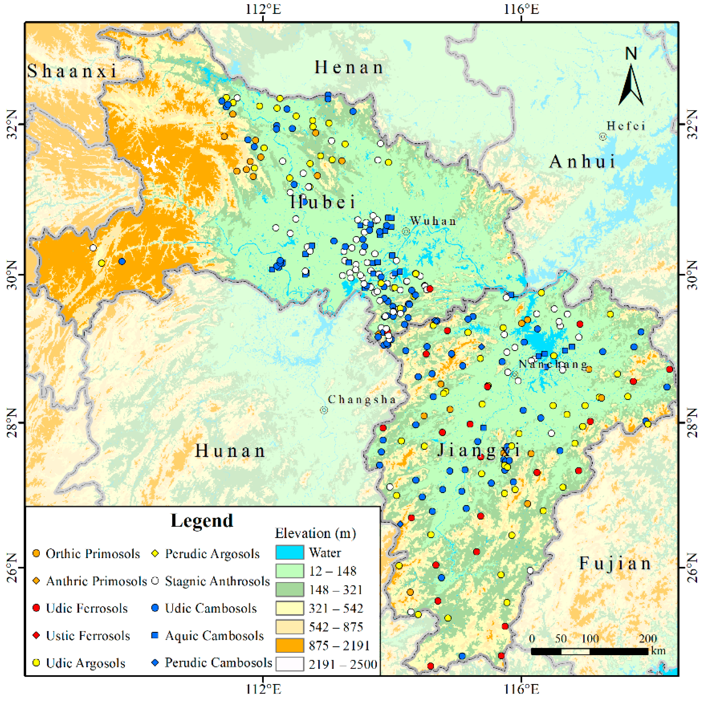
2.1. Study Area and Soil Profiles

The study area includes Hubei and Jiangxi Provinces in China (24°29′–33°20′ N, 108°21′~118°28′ E), as shown in Figure 1. Both provinces are in a humid subtropical monsoon climate, with abundant water and heat resources to meet the conditions for a wide range of crops, and most of the arable land in the region can grow two or three crops a year. There exists a full range of landscape types, with the Jianghan Plain located within the territory, the Yunnan–Guizhou Plateau in western Hubei and a small area of the Qinling Mountains, and the hilly areas in southern Jiangxi, which are more closely related to the formation and distribution of soils.

A total of 331 soil profiles were used, and the geographical distribution of the individual profiles is shown in Figure 1. These profiles were classified into a total of 10 soil suborders. The numerical distribution is shown in

Table 1. Suborders to which the soil at the profile sampling site belongs.

Order	Suborder	Number of Profiles	Total
Primosols	Orthic Primosols	22	23
	Anthric Primosols	1
Ferrosols	Udic Ferrosols	24	25
	Ustic Ferrosols	1
Argosols	Udic Argosols	64	65
	Perudic Argosols	1
Anthrosols	Stagnic Anthrosols	89	89
Cambosols	Udic Cambosols	96	129
	Aquic Cambosols	29
	Perudic Cambosols	4

.

The sampling sites in Hubei Province are concentrated in the southeastern and northerly parts of the province, mainly due to the high mountainous terrain in the western part of Hubei Province. The sampling sites in Jiangxi Province are more evenly distributed in all regions of the province. The sampling sites for Anthrosols and Cambosols in Hubei Province are concentrated in the southeastern part of the province’s plains, whereas the sampling sites for Argosols and Primosols are concentrated in the hilly and alpine parts of the province due north. The Ferrosols sampling sites in both provinces are largely located within Jiangxi Province, whereas the Anthrosols sampling sites in Jiangxi Province are mostly concentrated in the cultivated areas near the lacustrine plain of Poyang Lake.

Given the uneven distribution of soil resources within the study area, the number of profile sampling points within each category is not guaranteed to be evenly distributed. Table 1 has been ranked in ascending order of the number of profiles, from least to most, as Primosols, Ferrosols, Argosols, Anthrosols, and Cambosols.

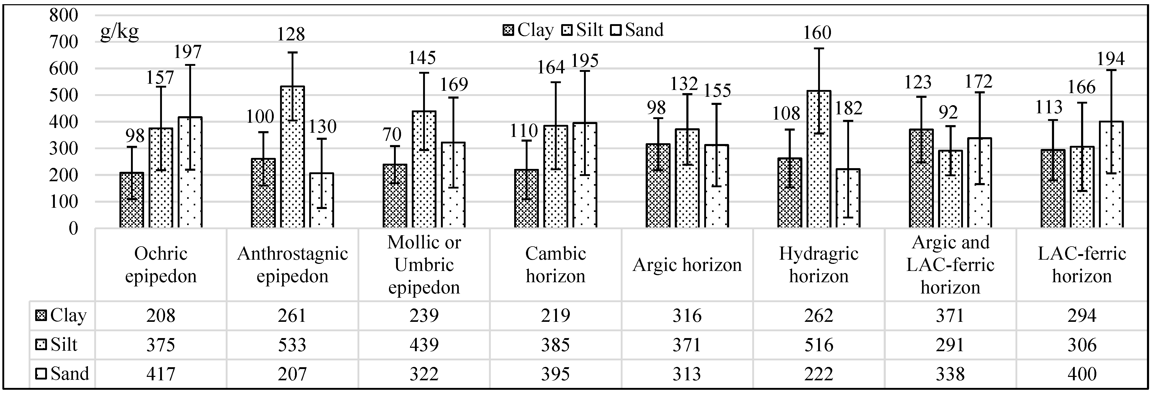
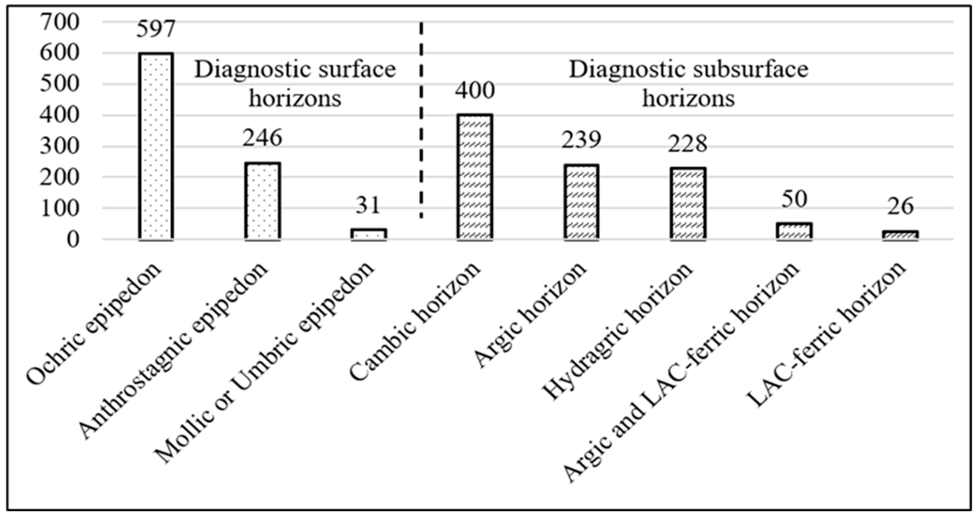
2.2. Categories Distribution, Morphological Attributes, and Physico-Chemical Properties of Soil Diagnostic Horizons

To obtain a general overview of the diagnostic horizons in this study, we generated categories distribution, morphological attributes, and physico-chemical properties of soil diagnostic horizons. They will help us to understand and discuss the ability of the model to identify different diagnostic horizons, and these attributes and properties can be directly characterized in RGB images.

Soil diagnostic horizons can be differentiated into diagnostic surface horizons and diagnostic subsurface horizons according to their position in the individual soil body. The distribution of the number of soil diagnostic horizons at the sampling sites in the study area is shown in Figure 2.

As shown in Figure 2, some categories only have one or two cases in the soil profile sample of this study. These categories were excluded to avoid interference in the model. Therefore, the categories of diagnostic horizons that were ultimately used include a total of eight categories: Ochric epipedon, Anthrostagnic epipedon, Mollic or Umbric epipedon, Cambic horizon, Argic horizon, Hydragric horizon, Argic and LAC-ferric horizon, and LAC-ferric horizon.

Morphological attributes that are clearly characterized in RGB images include the thickness, boundary, and root, as shown in

Table 2. The thickness, boundary, and root description of each diagnostic horizon. Boundary distinctness represents the thickness of the intersection region between a horizon and the one below it (abrupt: <2 cm, clear: 2–5 cm, gradual: 5–12 cm, and diffuse: ≥12 cm). Boundary topography was divided in the same way as in US Soil Taxonomy (ST). The highest percentage of each category is marked in red.

Diagnostic Horizon	Thickness Mean (cm)	Boundary Distinctness	%	Boundary Topography	%	Density of Roots (/dm2)	%	Thickness of Roots (mm)	%
Ochric epipedon	23	Abrupt	4%	Smooth	66%	0	3%	0	3%
		Clear	44%	Wavy	27%	1–20	13%	<0.5	9%
		Gradual	38%	Irregular	6%	20–50	40%	0.5–2	70%
		Diffuse	14%	Broken	1%	50–200	35%	2–5	16%
						≥200	9%	5–10	2%
Anthrostagnic epipedon	31	Abrupt	23%	Smooth	89%	0	6%	0	6%
		Clear	42%	Wavy	10%	1–20	5%	<0.5	9%
		Gradual	30%	Irregular	1%	20–50	25%	0.5–2	85%
		Diffuse	5%	Broken	0%	50–200	50%	2–5	0%
						≥200	14%	5–10	0%
Mollic or Umbric epipedon	26	Abrupt	0%	Smooth	55%	0	9%	0	9%
		Clear	45%	Wavy	45%	1–20	0%	<0.5	9%
		Gradual	55%	Irregular	0%	20–50	46%	0.5–2	64%
		Diffuse	0%	Broken	0%	50–200	18%	2–5	9%
						≥200	27%	5–10	9%
Cambic horizon	67	Abrupt	8%	Smooth	65%	0	21%	0	21%
		Clear	27%	Wavy	28%	1–20	33%	<0.5	18%
		Gradual	42%	Irregular	4%	20–50	35%	0.5–2	53%
		Diffuse	23%	Broken	3%	50–200	10%	2–5	5%
						≥200	1%	5–10	3%
Argic horizon	62	Abrupt	3%	Smooth	58%	0	14%	0	14%
		Clear	28%	Wavy	30%	1–20	40%	<0.5	28%
		Gradual	45%	Irregular	12%	20–50	33%	0.5–2	48%
		Diffuse	24%	Broken	0%	50–200	11%	2–5	6%
						≥200	2%	5–10	4%
Hydragric horizon	74	Abrupt	19%	Smooth	86%	0	44%	0	44%
		Clear	29%	Wavy	10%	1–20	25%	<0.5	12%
		Gradual	34%	Irregular	4%	20–50	21%	0.5–2	44%
		Diffuse	18%	Broken	0%	50–200	9%	2–5	0%
						≥200	1%	5–10	0%
Argic and LAC-ferric horizon	48	Abrupt	0%	Smooth	62%	0	6%	0	6%
		Clear	44%	Wavy	19%	1–20	38%	<0.5	38%
		Gradual	31%	Irregular	19%	20–50	38%	0.5–2	37%
		Diffuse	25%	Broken	0%	50–200	18%	2–5	13%
						≥200	0%	5–10	6%
LAC-ferric horizon	54	Abrupt	0%	Smooth	68%	0	12%	0	12%
		Clear	26%	Wavy	11%	1–20	11%	<0.5	23%
		Gradual	48%	Irregular	11%	20–50	44%	0.5–2	43%
		Diffuse	26%	Broken	0%	50–200	22%	2–5	22%
						≥200	11%	5–10	0%

.

The Munsell color system can be used to describe the color through various dimensions such as hue, value, and chroma. CST conventionally distinguishes soil diagnostic horizons based on hue. Soil moisture status affects soil color; as such, to ensure comparable assessment of soil color, the hue was recorded for moist soil, which is also the most common status of soils in the study area (

Table 3. Distribution of hue (moist) of each category of diagnostic horizons.

	Hue (Moist)	5R	7.5R	10R	2.5YR	5YR	7.5YR	10YR	2.5Y	5Y	7.5Y	10G	10BG	5PB	Total
Diagnostic Horizons
Ochric epipedon		1	1	3	27	47	85	41	2		1			1	209
Anthrostagnic epipedon					1	9	18	45	3	3			1		80
Mollic or Umbric epipedon					2	3	4	2							11
Cambic horizon				5	22	25	56	31	3	1					143
Argic horizon			2	1	19	28	24	10							84
Hydragric horizon					3	7	18	40	2	3		2	2		77
Argic and LAC-ferric horizon					6	7	2	1							16
LAC-ferric horizon				1	2	5		1							9
Total		1	3	10	82	131	207	171	10	7	1	2	3	1	629

). It was determined based on the Munsell soil-color charts [24], and corresponds directly to the values of the three bands in RGB images.

The soil texture of each diagnostic horizon was expressed by the content of clay (<0.002 mm), silt (0.002–0.05 mm), and sand (0.05–2 mm) based on USDA standards (Figure 3). Soil particle size distribution was measured using the pipette method [25].

The statistical information of soil free iron oxide content and soil organic carbon (SOC) content in soil chemical properties is shown in Figure 4. Soil free iron oxide content and SOC content was determined by the citrate bicarbonate dithionite (CBD) procedure [26] and the external-heat potassium dichromate oxidation-colorimetric method [27], respectively. The higher their value, the redder or darker the soil color will tend to be.

2.3. Image Dataset of Soil Diagnostic Horizons

The RGB images used in this study were all taken during field surveys with a Nikon digital single-lens reflex camera (model: D90) with a Nikon AF-S DX NIKKOR 18–105 mm f/3.5–5.6 G ED VR lens, with a maximum resolution of 2880 × 4032 pixels. As several images were taken for a single soil profile, significant differences exist in angle, light intensity, and camera parameters, so they were retained in the data processing for this study to improve the generalizability of the model. The final number of diagnostic horizons contained in all images is shown in Figure 5.

To intuitively feel the characteristics and differences between different categories of soil diagnostic horizons from the RGB image, the original soil profile image was cropped, and six pieces of more typical differences among different categories were selected, as shown in Figure 6. Notably, the figure is only for display and not the actual operation in semantic segmentation.

As shown in Figure 6, the diagnostic horizons have fewer common features characterized in the images, making it difficult to determine the category to which the diagnostic horizons belong, especially Ochric epipedon and Cambic horizon. Features of the soil diagnostic horizons that can be perceived by the human eye include:

(1)

Anthrostagnic epipedon tend to be yellowish or grayish in color and show a visual representation of gleying due to their agitation by rice farming activities.

(2)

The color of Hydragric horizon is mainly similar to Anthrostagnic epipedon, and it has a distinct redox characteristic, dominated by rust streak and rust spots.

(3)

Mollic or Umbric epipedon is generally darker in color; it also has more internal roots due to its higher organic carbon content.

(4)

The color of LAC-ferric horizon and Argic and LAC-ferric horizon tends to be reddish.

Although these diagnostic horizons have these common characteristics, individual samples from other diagnostic horizons also exhibit similar characteristics. Therefore, direct differentiation of the original image by the human eye alone is prone to recognition errors, and a deep learning model is required.

Before being inputted into the deep learning network, the images need resizing, data augmentation, and image labeling to form a standard image dataset. During the image resizing process, all RGB images were resized to 256 × 256 pixels depending on the computer memory configuration and other hardware conditions.

2.3.1. Data Augmentation

Deep learning often requires a large amount of data to train a model with good performance [28,29]. Data augmentation is often used to solve the problem of insufficient data. Various digital image processing operations (e.g., flipping, rotating, and brightness adjustment) are performed on the original image during data augmentation [30,31,32]. Such transformations can significantly increase the diversity of the training image and will thus also improve the performance of image segmentation [33,34] and prevent overfitting of the model [35,36].

The following methods were used for data augmentation, considering the various conditions that occur in the field when shooting with ordinary digital cameras, the characteristics of the profile images, and the characteristics of the original dataset.

(1)

Translation and rotation: Given the difficulty of photographing perfectly upright in the field and the susceptibility of researchers to shaking, data enhancement was limited to a percentage shift of less than 5% and an angle of less than 5°.

(2)

Flip: The profile images were all taken with the surface vegetation on top and from the top down, so only horizontal flips were considered.

(3)

Adjusting brightness: In view of the inconsistent lighting conditions at the time of shooting, brightness was adjusted appropriately to simulate different sunlight intensities.

The before and after changes in data augmentation are shown in Figure 7. The addition of noise perturbation was not considered because the current camera technology is considered to be quite mature in this study, and having a wide coverage of pepper noise and Gaussian noise is difficult. Moreover, it was also not considered for the process of adding color balance, because it was already achieved by adjusting the camera parameters during the field survey.

Randomly applying different translation, rotation, and brightness adjustment values to the images of the 331 soil profiles, as well as randomly performing horizontal flips, resulted in 10 images for each profile. Given that many images came from the same profile, we distinguished the training dataset images from the validation dataset images by the ID number of the soil profiles, which means that all the images generated by each soil profile can only exist in the training or validation dataset. The final result was a dataset of 2320 training images and 990 validation images. The ratio of the number of training images to the number of validation images was 7:3.

2.3.2. Image Labeling

For semantic segmentation algorithms, image labeling is a necessary step for training a supervised model [37,38]. In this step, all diagnostic horizons are manually delineated using the Labelme software package [39] based on existing soil profile descriptions. The input images for labeling are those that have undergone resizing and data augmentation. A total of 3310 images needed to be image-labeled for this study. The manual delineation process attempted to avoid delineating the hanging plant leaves in the surface horizons. The specific boundaries between horizons were delineated by reference to their clear soil profile original images. When distinctness of the boundary of a soil diagnostic horizon is considered diffuse in the field survey description of the soil profile, it would then be delineated by a straight line based on depth information with the soil profile ruler in the image. This is because the inherently diffuse boundaries are more difficult to accurately delineate manually after image compression. This process completes the construction of the image database for the soil diagnostic horizons.

2.4. Semantic Segmentation Network Model-UNet++

The UNet++ model (Figure 8) is an improved model based on U-Net model [40]. Its advantage is that further learning of the different layers of the convolution process without deepening the network layers makes UNet++ have a better fine-grained segmentation capability compared with U-Net [41]. At the same time, it also has the same advantage in accuracy performance in relatively small datasets that the U-Net model does compared with other classical semantic segmentation models [42,43].

The original image was downsampled four times in the encoder path (Figure 8a), with convolution, activation function, and maximum pooling performed at each layer. As the number of layers progresses deeper, the resolution of each layer feature map gradually becomes lower; the image is gradually blurred and abstracted; the number of channels gradually increases; and detailed information, such as spatial localization features, is gradually lost, but more image features are extracted [44]. Different from CNNs, the decoder path (Figure 8b) of UNet++ used the feature map to perform the corresponding four layers of upsampling, recovering the compressed image up to restoration and outputting the segmented image [45]. To fuse more of the shallow feature information, the symmetric encoder was also channel-merged with the feature maps on the decoder path via skip paths (the black dashed lines in Figure 8), and the features extracted during downsampling were passed directly into the upsampling, thereby adding more details [46].

UNet++, a variant, innovative architecture of U-Net, further connected the feature maps on the encoder and decoder paths through more densely nested skip paths (the green part in Figure 8). In this pathway all nodes in L1 to L5 could be connected by upsampling at each layer, and more feature information was thus fused [47]. Nested skip paths were also used to transfer information from each node in the encoder path to the decoder path for the input image [48]. The original images generated by sampling reductions from multiple decoder branches (the four images in Figure 8d) are the result of multiple cascade skip paths. Finally, all output images from multiple decoder branches were averaged to obtain the final segmentation result [40].

The symmetrical code network architecture complements the semantic information of the input image by extrapolating the missing image information through mirror folding [49]. The skip connection allows the feature maps in the encoder and decoder to be fused directly; and the deep detailed information embedded in the image and the superficial semantic information revealed can thus be obtained and aggregated more efficiently [50]. This network architecture would therefore be well suited to relatively small datasets and for studies with high fine-grained requirements and thus fits the needs of this study.

2.5. Model Validation Indicators

In the quantitative assessment of the model, the previously manually delineated horizons based on the description of the soil profile were considered to be the true results. All validation indicators would be performed at the pixel level. In studies related to semantic segmentation, loss functions are mostly used for the convergence of the model, whereas for the final evaluation of the model, mean intersection over union (MIoU) and pixel accuracy (PA) are most widely used [51,52,53].

The intersection over union (IoU) is the ratio between the intersection area of the true values of the pixels in the image (manually delineated regions) and the predicted values (automatically delineated regions by the model) and the union area of the two, calculated as shown in Equation (1) [54,55]. The MIoU is the mean value of IoU in a category and is calculated as shown in Equation (2) [54,55]. This indicator primarily quantifies the similarity between the predicted results and the manually delineated horizon.

$$IoU=\frac{P\cap G}{P\cup G}$$

(1)

$$MIoU=\frac{{\displaystyle \sum }Io{U}_i}{n}$$

(2)

In Equation (1), $P$ refers to the prediction of the model, $G$ refers to the manually delineated area, $P\cap G$ refers to the area of the intersection of $P$ and $G$, and $P\cup G$ refers to the area of the union of $P$ and $G$. In Equation (2), $\sum Io{U}_i$ is the sum of IoU at a particular soil horizon category, and $n$ is the number of samples in the category.

PA is the ratio of correctly segmented pixels to the total number of pixels in the image, reflecting the accuracy of the model, calculated as shown in Equation (3) [54,55].

$$PA=\frac{TP+TN}{TP+FP+TN+FN}$$

(3)

TP (True Positive) indicates the number of cases that the model predicts as Positive (P), which are actually Positive, so the prediction is correct (True, T); whereas FN (False Negative) indicates that the model predicts Negative (N), which is actually the number of Positive cases, so the prediction is incorrect (False, F). With this rule, TN represents the number of cases predicted as N but correctly judged as N, and FP represents the number of cases predicted as P but incorrectly judged as N.

In deep learning, if there exists a serious imbalance in the number of samples between categories, the neural network will focus on learning images of categories with a large number of samples and ignore those with a small number of samples; this imbalance will cause a huge difference in the value of the loss function for each category of data, which eventually leads to a skewed distribution of recognition ability for each category [56]. In this study, as the input image is a whole image, the number of diagnostic horizons contained in each image is inconsistent. Thus, equalizing the diagnostic horizon samples through data augmentation is difficult. This problem tends to arise in the field of semantic segmentation. A more effective way to solve this problem is to adjust the loss function. In this study, a loss function called Unified Focal Loss Function, which is a combination of Dice loss function and Focal loss function, is used as a new hierarchical framework to deal with the class imbalance [57]. It combines functionally equivalent hyperparameters and uses asymmetry to focus the suppression and enhancement of the focal parameters on the modified loss components [57].

2.6. Model Training

This study is based on the PyTorch deep learning framework for model training, with an Intel Xeon central processing unit and an NVIDIA GeForce RTX 3060 laptop GPU with 6 GB of memory.

During the training process, the learning rate (LR) in the training parameters was 0.001, and it was set to changeable (it would judge whether there exists progress during training based on the loss function of the validation dataset and gradually reduce the LR to make the model perform better). The batch size was set to 4 due to the small gigabytes of memory of the GPU for this study, and epoch was chosen to be 150 after several pretests.

3. Results

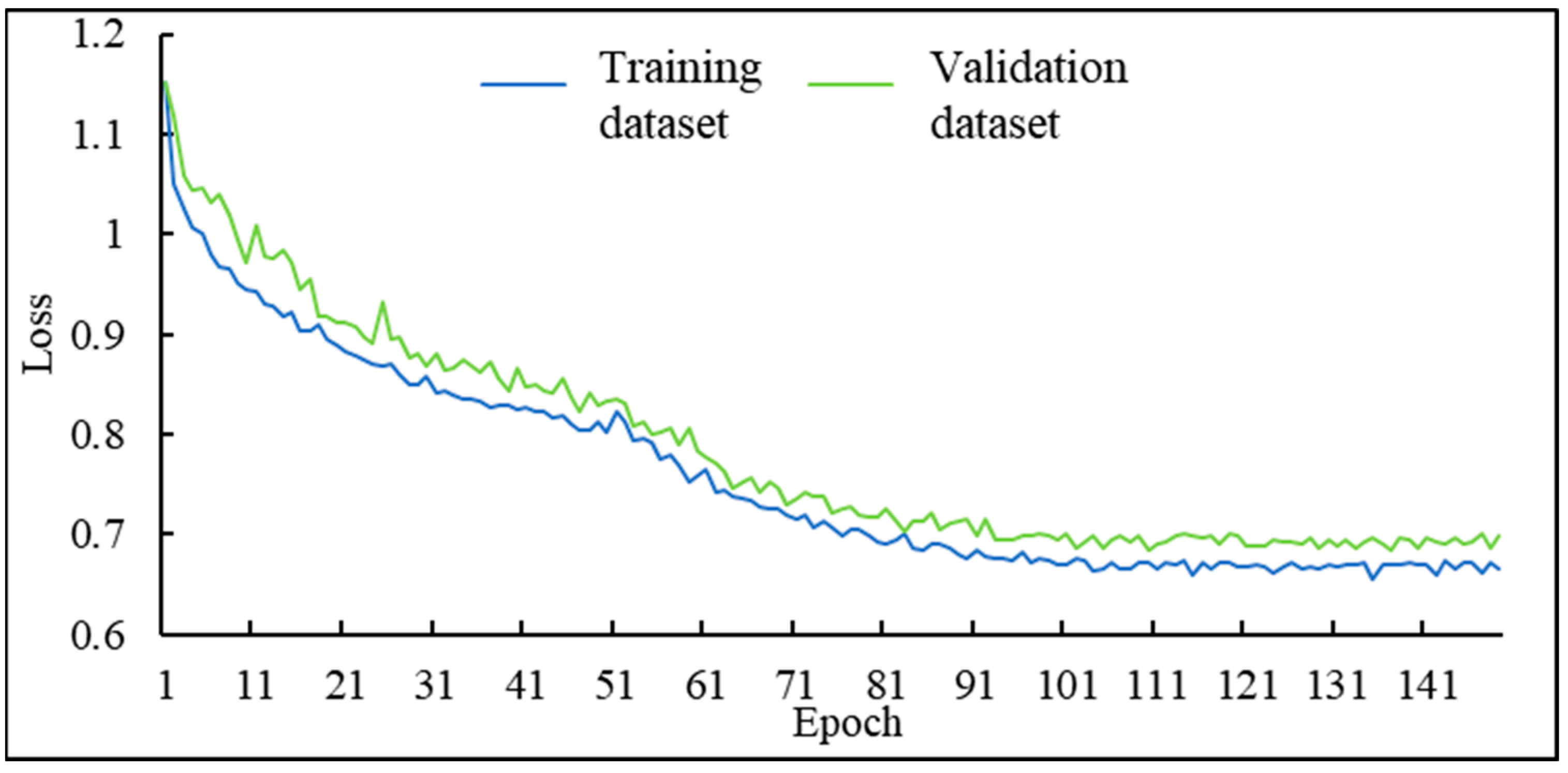
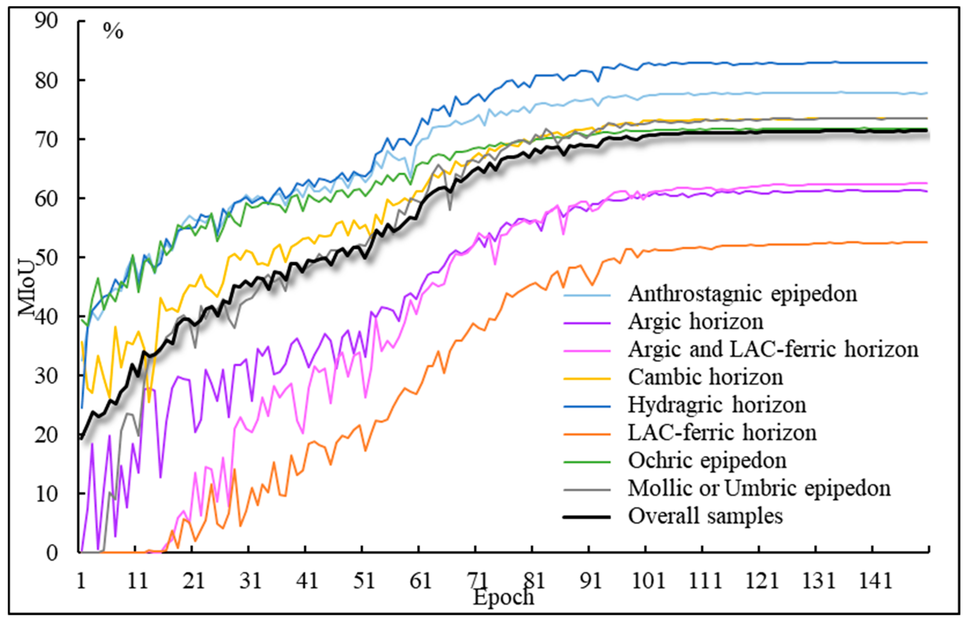
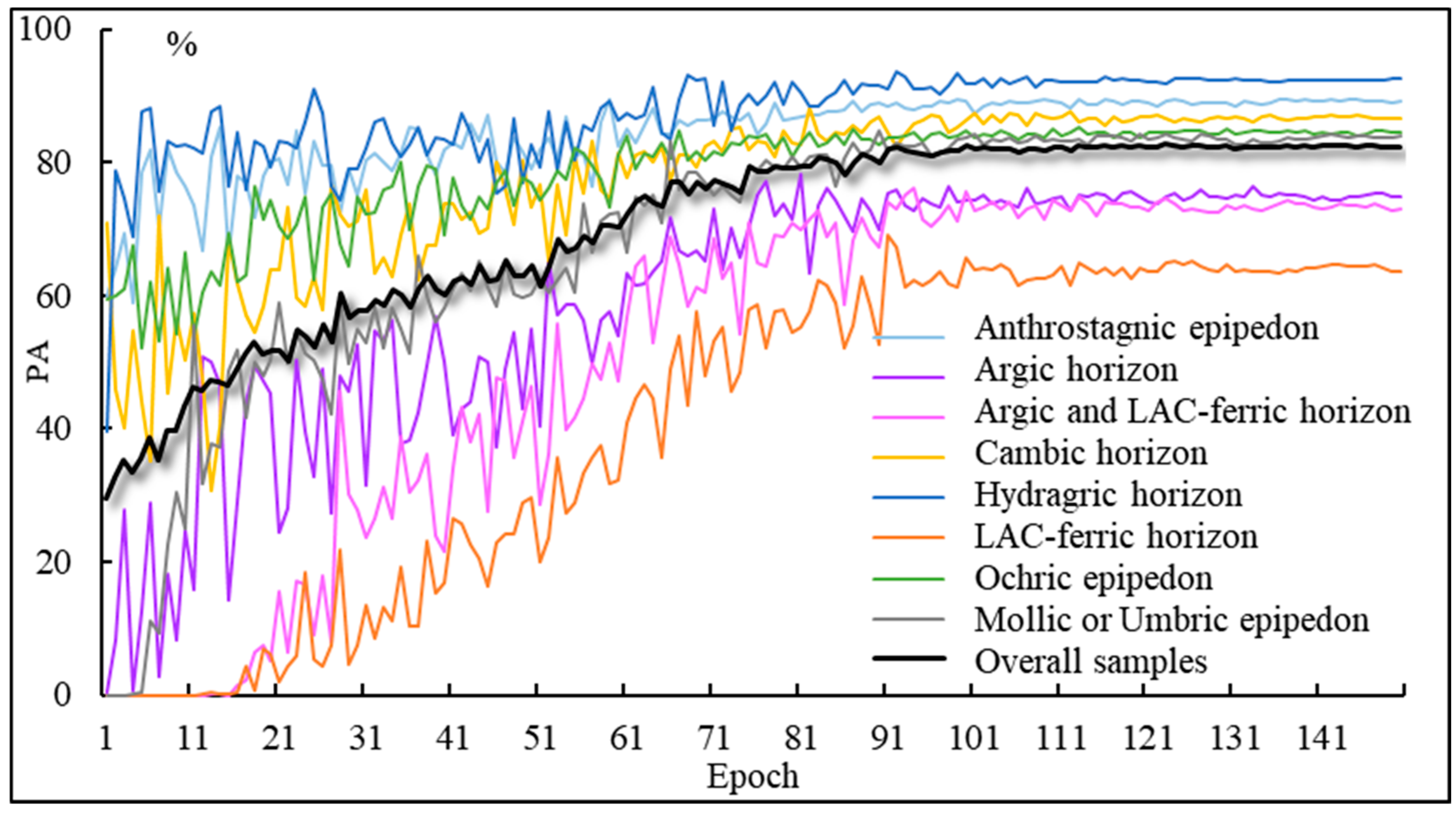
3.1. Training Process

After inputting the 3310 images through preprocessing into the UNet++ model, the loss curves of the training and validation datasets during the model training are shown in Figure 9.

The model generally converged throughout the 150 epochs, with the value of the loss function decreasing in general. The loss curves on the training and validation datasets decreased slowly from the first to the 100th epoch and leveled off between the 100th and 150th epochs. The number of epochs to reach a plateau in the loss curve was approximately the same for both datasets, and the curve converges with relatively less fluctuation. In addition, the value of the loss function in the training dataset stabilized at roughly 0.66 ± 0.01 after the 100th epoch and was at its lowest value of 0.655 at the 135th epoch, whereas the value of the loss function in the validation dataset stabilized at roughly 0.68 ± 0.01 after the 100th epoch and was at its lowest value of 0.683 at the 137th epoch. However, the lowest value of the loss function does not indicate that the performance of the model is optimal at this time.

Accordingly, the MIoU curves of different diagnostic horizon categories for all samples (including the training and validation datasets) and the MIoU curves for the overall samples (all diagnostic horizon categories for all datasets) during the training process were plotted, as shown in Figure 10. Before the 50th epoch, the model performed better in the MIoU of the three categories of diagnostic horizons, namely, the Ochric epipedon, Anthrostagnic epipedon, and Hydragric horizon, with a higher differentiation ability. However, the MIoU curves of the three intersected one another and were difficult to differentiate, and the MIoU of the three was not significantly different at this time. Moreover, the MIoU from high to low for the remaining diagnostic horizons were Cambic horizon > Mollic or Umbric epipedon > Argic horizon > Argic and LAC-ferric horizon > LAC-ferric horizon. From the 50th to the 70th epoch, the MIoU curves of the three types of diagnostic horizons, namely the Ochric epipedon, Anthrostagnic epipedon, and Hydragric horizon, were gradually separated, and the MIoU from high to low was Hydragric horizon > Anthrostagnic epipedon > Ochric epipedon. The MIoU curves of the Cambic horizon and the Mollic or Umbric epipedon, and the Argic horizon and the Argic and LAC-ferric horizon gradually moved closer to each other. The MIoU of the LAC-ferric horizon remained the worst performer. After the 70th epoch, the MIoU curve for the Ochric epipedon had plateaued and was intersected by the Cambic horizon and the Mollic or Umbric epipedon, and was gradually lower than the latter two. After the 100th epoch, the MIoU curves for all horizons and the overall samples had smoothed out, and the MIoU for the different diagnostic horizon categories were Hydragric horizon > Anthrostagnic epipedon > Mollic or Umbric epipedon ≈ Cambic horizon > Ochric epipedon > Argic and LAC-ferric horizon > Argic horizon > LAC-ferric horizon, with the highest values for each diagnostic horizon corresponding to 82.98%, 77.86%, 73.54%, 73.45%, 71.79%, 62.44%, 61.37%, and 52.52%, respectively. The overall samples reached their highest value of 71.36% in the 148th epoch.

Different from the change curve of MIoU, which converged upward with relatively small fluctuations, the change curve of the PA (Figure 11) of each diagnostic horizon category apparently fluctuated relatively more drastically in the early stages of the model training; however, it still generally followed an upward convergence trend and was relatively smoother in the later stages of the training. Similar to the MIoU, the PA curves reached a plateau at the 100th epoch of the model training. The order of PA for each diagnostic horizon category from largest to smallest was broadly similar to the MIoU, with Hydragric horizon > Anthrostagnic epipedon > Cambic horizon > Ochric epipedon > Mollic or Umbric epipedon > Argic horizon > Argic and LAC-ferric horizon > LAC-ferric horizon. The highest values for each of its diagnostic horizons corresponded to 93.71%, 89.55%, 88.09%, 85.38%, 84.79%, 78.31%, 76.08%, and 69.10%. The overall samples reached their highest PA value of 82.66% in the 123rd epoch.

The number of epochs when the two validation indicators MIoU and PA reached their maximum were not the same, the 148th and 123rd epochs, respectively. The models generated from these epochs should represent the most accurate model for identifying the soil diagnostic horizons in terms of their respective validation indicators. To combine the effects of the two validation indicators to select the final model, the indicators of the models generated by the 148th and 123rd epochs for each samples were counted, as shown in

Table 4. Different metrics of the models generated in the 123rd and 148th epochs. The standard deviation indicates the standard deviation of the corresponding indicator for all diagnostic horizons.

Epoch	123rd		148th
	MIoU (%)	PA (%)	MIoU (%)	PA (%)
Ochric epipedon	71.69	84.51	71.78	84.68
Cambic horizon	73.39	86.48	73.45	86.57
Mollic or Umbric epipedon	73.38	84.09	73.49	83.64
LAC-ferric horizon	52.16	64.95	52.49	64.01
Argic horizon	61.03	74.85	61.29	75.25
Anthrostagnic epipedon	77.80	89.23	77.74	89.08
Hydragric horizon	82.86	91.90	82.88	92.33
Argic and LAC-ferric horizon	62.19	74.53	62.43	73.15
Standard deviation	9.41	8.48	9.29	8.86
The overall samples	71.24	82.66	71.36	82.38
The sum of standard deviations	17.89		18.15
MIoU + PA	153.9		153.7

. The model produced by the 123rd epoch outperformed the 148th epoch in terms of the sum of standard deviations and MIoU + PA. The model generated in the 123rd epoch was therefore chosen as the final model.

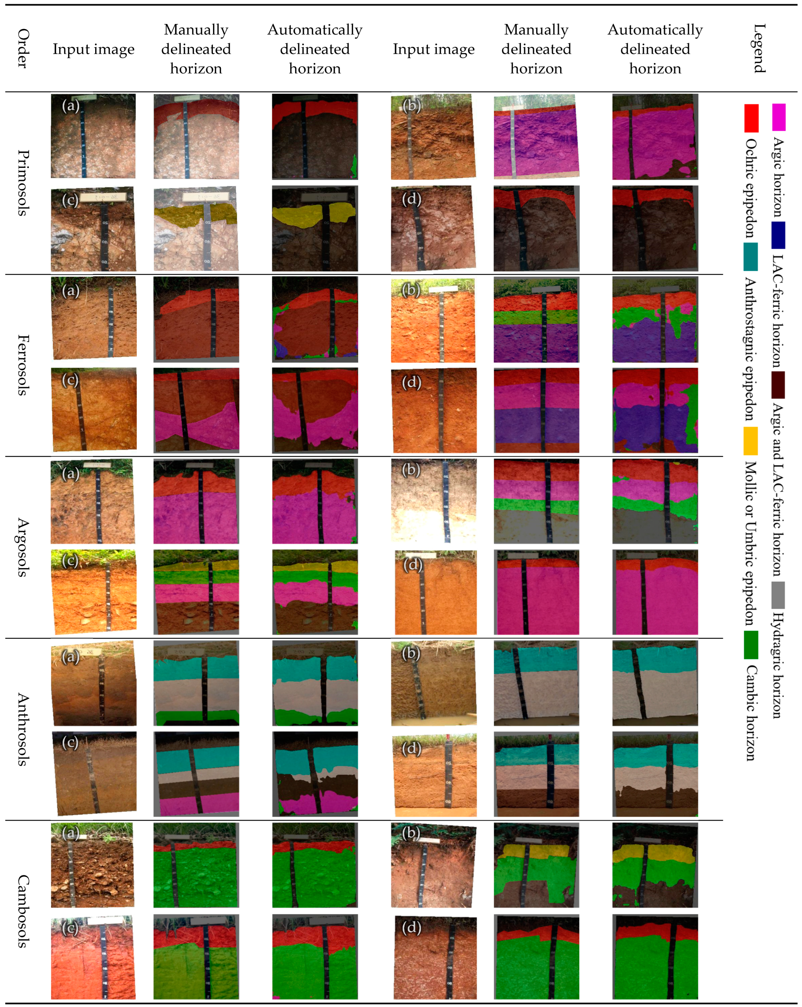
3.2. Model Validation

The manually delineated labels from the field description data were considered to be true and correct for the location and category of horizons. As previously described, diffuse boundaries were represented with straight lines, and such processing will increase the uncertainty of manual delineation, and therefore of model validation.

The order in which the model’s ability to identify different soil diagnostic horizon categories based on the validation indicators was shown in Figure 12. To explore the shortcomings of the model obtained from training and to observe the model run results more visually, four representative soil profile images from each of the five soil orders were selected as input images (images after image augmentation) into the model. Then, the manually delineated images with labels were compared with the model identification result images and finally displayed as an example, as shown in Figure 13. In Argosols (b), the bottom overexposure was attributed to the presence of a large amount of reflective sand in the parent material horizon. Based on the image color, some boundaries of diagnostic horizons, i.e., Anthrosols (a,c), seemed to be overlooked. This is because the horizons that appeared to exist had been analyzed by the laboratory and belonged to the same category of diagnostic horizon based on CST.

In combination with Figure 12 and Figure 13, in general, the UNet++-based soil diagnostic horizon identification model could identify and delineate the soil diagnostic horizon categories covered in the study accurately, with an MIoU of 71.24% and an average PA of 82.66%.

In Figure 12 and Figure 13, the Hydragric horizon and the Anthrostagnic epipedon showed the highest recognition ability on both validation indicators. Moreover, the boundaries between them and the water surface in the soil pits, and the background (i.e., vegetation above the surface horizon) could be delineated accurately on the images.

The Cambic horizon, Mollic or Umbric epipedon, and Ochric epipedon were identified second to the Hydragric horizon and Anthrostagnic epipedon. Particularly, the Ochric epipedon was accurately identified by the model even when they occurred in thinner soil thicknesses, as shown in Figure 13 for the Primosols (b). Many images of Cambic horizon of varying sizes appeared incorrectly as patches in the images of various categories of soil, as shown in Figure 13 for Primosols (a,d), Ferrosols (a,d), Argosols (a), and Anthrosols (c).

The model’s ability to identify the Argic and LAC-ferric horizon, the Argic horizon, and the low LAC-ferric horizon was poor, with the MIoU and PA for the LAC-ferric horizon being only 52.16% and 64.95%, respectively, which were considerably lower than the other diagnostic horizons. In Figure 13, the area of images in Ferrosols was more confusing than in other soil categories, particularly in Ferrosols (a,d), where there existed an even larger area of horizon categories that did not exist in their corresponding manually delineated images. In contrast, in the Argosols, the Argic horizon was better delineated and identified.

When the boundaries between soil horizons were more diffuse, the delineation is less effective. This phenomenon was particularly prominent in the Ferrosols (b,d) and the Anthrosols (c) in Figure 13.

4. Discussion

4.1. Analysis of Misclassifications

Soil diagnostic horizon delineation and identification, as one of the practical applications of semantic segmentation algorithms, is more challenging than semantic segmentation applications in other fields due to boundary ambiguity and the existence of broken boundary shapes. However, generally, the images obtained from the diagnostic horizon identification model can still provide realistic and accurate information on the categories and location of diagnostic horizons, providing fast, efficient, and inexpensive technical support for diagnostic horizon delineation and identification.

For all the roots and stones contained in the images, we consider that they are important references for identifying the categories of soil diagnostic horizons; for example, where there are many roots tends to be diagnostic surface horizons, and where there are many rice roots there tends to be the Anthrostagnic epipedon, as shown in Table 2. Meanwhile, those with many stones tend to be soils with weak soil development, such as the Primosols and the Cambosols, and this type of soil tends to have only a very thin diagnostic surface horizon. For instance, the Ochric epipedon, as shown in Table 2, has the thinnest average thickness.

As there tends to be a large difference between the top and bottom of the soil profile image, the ability of the model to identify diagnostic surface horizons differed from diagnostic subsurface horizons. In terms of validation indicators, the diagnostic surface horizons were easier to identify compared with the diagnostic subsurface horizons due to the fact that surface soils are usually darker in color, as shown in Figure 6, associated with the accumulation of humified organic matter (corresponded to their apparently high SOC content in Figure 4) and thus differ more from the diagnostic subsurface horizons [58]. This result is also consistent with the findings of Jiang et al. [18].

For the two important diagnostic horizons of the Anthrosols, the Hydragric horizon and the Anthrostagnic epipedon, after traversing all the images of the model identification results, the two diagnostic horizons were hardly present in the identification results of other soil categories. The reason was that the two horizons were distinguished from the others by their distinctive image characteristics, as analyzed in Section 2.3. Such characteristics include tending to be more yellow or gray in color (corresponding to their main hues concentrated in 10YR in Table 3) and having stronger visual representations, such as gleying and redox characteristics due to the effects of long-term rice farming activities.

Section 3.2 of this paper mentioned that areas in the various soil profiles were frequently incorrectly classified as Cambic horizon. The Cambic horizon is defined as a soil horizon with soil structure development, essentially without material deposition, without obvious claying, with red, yellow, purple, and brown colors. The characteristics of Cambic horizons commonly seen in Hubei and Jiangxi Regions can be summarized as: (1) finer texture; (2) fine earth fraction (<2 mm) occupies more volume than coarse fragments; (3) a higher degree of color; and a relatively more red or yellow hue than the bottom horizons; and (4) not meeting the conditions of Argic horizon or LAC-ferric horizon [59]. Its characteristics apply in a relatively broad range and can easily be misclassified in other soil categories. In addition, Table 2 and Table 3, Figure 3, Figure 4, and Figure 6 highlight the difficulty in identifying Cambic horizons.

The Ochric epipedon was similar to the Cambic horizon in that it applied in a broad range of visual characteristics that can be extracted from its definition. It is defined as a relatively poorly developed, lighter colored, or thinner humus surface horizon [59]. However, the Ochric epipedon was accurately classified by the model due to its belonging to the diagnostic surface horizon and the large difference between it and the diagnostic subsurface horizon. In addition, the distinctness of their boundaries was mostly clear in Table 2.

The Mollic or Umbric epipedon were better identified by the model due to their relatively darker color and abundance of roots. Specifically, in Table 2, the root density was generally more than 20/dm²; in Figure 4, both soil free iron oxide and SOC content were relatively high, with the highest content of SOC.

For the soils in the study area in Hubei and Jiangxi Provinces, the claying and feralization of some of the soil profiles in the border area of the two provinces happened simultaneously [60]. Thus, there exist some diagnostic horizons that belong to Argic horizon and LAC-ferric horizon in the study area samples. This type of soil horizon was labeled as a different category of diagnostic horizon from the Argic horizon or LAC-ferric horizon in the image labeling to meet the practical requirements. This categorization (Argic and LAC-ferric horizon) also caused some interference in the model’s identification of the three diagnostic horizons: Argic horizon, LAC-ferric horizon, and Argic and LAC-ferric horizon (corresponding to them as very similar in Table 2 and Table 3, Figure 3 and Figure 4). The small number of samples of LAC-ferric horizons in the study area and the similarity of most diagnostic horizons to LAC-ferric horizons (Figure 6) are also considered to be the main reasons for the relatively low values of the validation indicators corresponding to the three diagnostic horizons.

4.2. Applicability Analysis to Other Taxonomic Systems

All soil categories and diagnostic horizons used in this study were obtained based on the CST, and these categories do not have exact one-to-one correspondence with other taxonomic systems. Therefore, the applicability of this method to other taxonomic systems needs to be analyzed.

In the development of CST, it was emphasized that its system was in line with international standards and fully drew on foreign classification experience. It claimed that 36.4% of the diagnostic horizons were directly quoted from the US Soil Taxonomy (ST), 27.2% were introduced concepts to be revised and supplemented, while 36.4% were newly proposed [59]. At the same time, it claimed that the newly proposed categories were classified according to the same principles and methods found in other systems (ST, Food and Agriculture Organization of the United Nations (FAO)/United Nations Educational, Scientific and Cultural Organization (Unesco), and World Reference Base) [59]. Therefore, the two systems are inherently relatively similar. At the same time, the deep learning method used in this study is based on a network that identifies and delineates diagnostic horizons of common features “learned” from manually drawn image regions, so we believe that this method is still feasible even for other taxonomic systems.

4.3. Comparison to Existing Studies

Soil morphological characterization based on soil profile imaging techniques is an area of great interest in soil science and has been extensively studied.

Devices commonly used for profile imaging include pXRF spectrometers [12], imaging spectrometers [13], DSLR cameras [15], smartphones [16], and so on. Although pXRF and vis-NIR sensors capture more information than RGB images from DSLR cameras or smartphones, the latter may be more appropriate for field soil surveys, especially for large-scale projects, because of cost effective, portable, and the low penetration rate.

Clustering approaches have been used to digitize soil morphological characteristics [17] and were shown to quickly and automatically delineate boundaries of soil horizons for soil profile images. However, this method cannot assign the category of horizon or epipedon to each region in the image. In addition, the clustering methods require a high requirement for image pre-processing [61]. For these reasons, the semantic segmentation method used in this study is advantageous. Moreover, in deep learning, the preprocessing of images is not complicated and the diversity of the original images improves the robustness of the model.

Jiang et al.’s study [18] also performed soil horizon delineation and identification based on deep learning with RGB images, but the final result of their identification was mainly A, B, and C categories. Our approach, which provides delineation and identification of diagnostic horizons, provides substantially more information. Furthermore, the number of samples was roughly balanced when segmenting the profiles into A, B, and C categories in the study by Jiang et al. [18], while the number of samples in the current study is severely imbalanced when segmenting soil profile images into diagnostic horizon categories (such as the LAC-ferric horizons). Due to the imbalance in our data, we chose a unique loss function to counteract this challenge. In addition, our study focuses on field soil surveys, and the difference from their study is reflected in data augmentation. Specifically, various noise disturbances as well as vertical flips were used in their study, while not in ours.

4.4. Limitations and Prospects

In this study, on the basis of the RGB profile images of the main soil categories in Jiangxi and Hubei Provinces, a soil diagnostic horizon identification model was obtained through deep learning model training. The model performed well in terms of accuracy and met the objectives of being fast, efficient, convenient, and inexpensive, which are required in field soil survey work. Moreover, the model is of great practical significance for the application and quantitative expression of soil information. However, there still exist limitations in the research process that need to be addressed in future studies:

(1)

Only soil profile image data from Hubei and Jiangxi Provinces were used in this study, resulting in a large limitation of identifiable categories. Meanwhile, the severe imbalance in different category samples, although suppressing the disappearance of some of the gradients by adjusting the loss function, did not completely resolve the problem and still had an impact on the small number of samples, such as the LAC-ferric horizon.

(2)

This study relied only on manual delineation when labeling soil diagnostic horizons, resulting in a large amount of data preprocessing. This study also has repeatedly emphasized that not all boundaries of soil diagnostic horizons are clear, which will have an impact on model training. Thus, future research is expected to automatically label images by image clustering to reduce the preprocessing workload.

(3)

Soil diagnostic horizon identification by RGB images alone cannot sufficiently reflect the physical and chemical properties of the soil. In the identification of diagnostic horizons where some diagnostic conditions have requirements for elemental content (e.g., LAC-ferric horizon), the identification and delineation of soil diagnostic horizons may still require the combined support of pXRF or vis-NIR spectroscopy to quantitatively reflect the variation of different soil chemical properties and elemental distributions in the profile.

5. Conclusions

In this study, a soil diagnostic horizon identification model based on a deep learning model and RGB images was developed to identify and delineate the diagnostic horizons of the main soil types in Jiangxi and Hubei Provinces. The study shows that the model validation indicators and the resultant images performed well, with MIoU of 71.24% and PA of 82.66%.

Moreover, the model’s ability to identify each diagnostic horizon was different depending on whether their visual features embodied in the images as defined in the CST were obvious and broad, as well as their respective sample sizes. Furthermore, the special case of simultaneous claying and feralization of soil profiles in parts of the study area had a considerable effect on the identification ability.

References

1. Xu, D.; Ma, W.; Chen, S.; Jiang, Q.; He, K.; Shi, Z. Assessment of Important Soil Properties Related to Chinese Soil Taxonomy Based on Vis–NIR Reflectance Spectroscopy. Comput. Electron. Agric. 2018, 144, 1–8. [Google Scholar] [CrossRef]
2. Shi, X.Z.; Yu, D.S.; Yang, G.X.; Wang, H.J.; Sun, W.X.; Du, G.H.; Gong, Z.T. Cross-Reference Benchmarks for Translating the Genetic Soil Classification of China into the Chinese Soil Taxonomy. Pedosphere 2006, 16, 147–153. [Google Scholar] [CrossRef]
3. Ju, B.; Wu, K.; Zhang, G.; Rossiter, D.G.; Li, L. Characterization of Some Calcareous Soils from Henan and Their Proposed Classification in Chinese Soil Taxonomy. Pedosphere 2017, 27, 758–768. [Google Scholar] [CrossRef]
4. Hartemink, A.E.; Zhang, Y.; Bockheim, J.G.; Curi, N.; Silva, S.H.G.; Grauer-Gray, J.; Lowe, D.J.; Krasilnikov, P. Soil Horizon Variation: A Review. Adv. Agron. 2020, 160, 125–185. [Google Scholar] [CrossRef]
5. Churchman, G.J. The Philosophical Status of Soil Science. Geoderma 2010, 157, 214–221. [Google Scholar] [CrossRef]
6. Yang, J.; Shen, F.; Wang, T.; Wu, L.; Li, Z.; Li, N.; Dai, L.; Liang, J.; Zhang, J. PEF-MODFLOW: A Framework for Preliminary Soil Profile Horizon Delineation Based on Soil Color Captured by Smartphone Images. Environ. Model. Softw. 2022, 155, 105423. [Google Scholar] [CrossRef]
7. Hartemink, A.E.; Minasny, B. Towards Digital Soil Morphometrics. Geoderma 2014, 230–231, 305–317. [Google Scholar] [CrossRef]
8. Kidd, D.; Searle, R.; Grundy, M.; McBratney, A.; Robinson, N.; O’Brien, L.; Zund, P.; Arrouays, D.; Thomas, M.; Padarian, J.; et al. Operationalising Digital Soil Mapping—Lessons from Australia. Geoderma Reg. 2020, 23, e00335. [Google Scholar] [CrossRef]
9. Sepuru, T.K.; Dube, T. An Appraisal on the Progress of Remote Sensing Applications in Soil Erosion Mapping and Monitoring. Remote Sens. Appl. Soc. Environ. 2018, 9, 1–9. [Google Scholar] [CrossRef]
10. Barra, I.; Haefele, S.M.; Sakrabani, R.; Kebede, F. Soil Spectroscopy with the Use of Chemometrics, Machine Learning and Pre-Processing Techniques in Soil Diagnosis: Recent Advances—A Review. TrAC Trends Anal. Chem. 2021, 135, 116166. [Google Scholar] [CrossRef]
11. Searle, R.; McBratney, A.; Grundy, M.; Kidd, D.; Malone, B.; Arrouays, D.; Stockman, U.; Zund, P.; Wilson, P.; Wilford, J.; et al. Digital Soil Mapping and Assessment for Australia and beyond: A Propitious Future. Geoderma Reg. 2021, 24, e00359. [Google Scholar] [CrossRef]
12. Sun, F.; Bakr, N.; Dang, T.; Pham, V.; Weindorf, D.C.; Jiang, Z.; Li, H.; Wang, Q.B. Enhanced Soil Profile Visualization Using Portable X-ray Fluorescence (PXRF) Spectrometry. Geoderma 2020, 358, 113997. [Google Scholar] [CrossRef]
13. Zhang, Y.; Hartemink, A.E. Soil Horizon Delineation Using Vis-NIR and PXRF Data. CATENA 2019, 180, 298–308. [Google Scholar] [CrossRef]
14. Ge, Y.; Chen, K.; Liu, G.; Zhang, Y.; Tang, H. A Low-Cost Approach for the Estimation of Rock Joint Roughness Using Photogrammetry. Eng. Geol. 2022, 305, 106726. [Google Scholar] [CrossRef]
15. Jiang, Z.D.; Wang, Q.B.; Brye, K.R.; Adhikari, K.; Sun, F.J.; Sun, Z.X.; Chen, S.; Owens, P.R. Quantifying Organic Carbon Stocks Using a Stereological Profile Imaging Method to Account for Rock Fragments in Stony Soils. Geoderma 2021, 385, 114837. [Google Scholar] [CrossRef]
16. Yang, J.; Shen, F.; Wang, T.; Luo, M.; Li, N.; Que, S. Effect of Smart Phone Cameras on Color-Based Prediction of Soil Organic Matter Content. Geoderma 2021, 402, 115365. [Google Scholar] [CrossRef]
17. Zhang, Y.; Hartemink, A.E. A Method for Automated Soil Horizon Delineation Using Digital Images. Geoderma 2019, 343, 97–115. [Google Scholar] [CrossRef]
18. Jiang, Z.D.; Owens, P.R.; Zhang, C.L.; Brye, K.R.; Weindorf, D.C.; Adhikari, K.; Sun, Z.X.; Sun, F.J.; Wang, Q.B. Towards a Dynamic Soil Survey: Identifying and Delineating Soil Horizons in-Situ Using Deep Learning. Geoderma 2021, 401, 115341. [Google Scholar] [CrossRef]
19. Ganaie, M.A.; Hu, M.; Malik, A.K.; Tanveer, M.; Suganthan, P.N. Ensemble Deep Learning: A Review. Eng. Appl. Artif. Intell. 2022, 115, 105151. [Google Scholar] [CrossRef]
20. Mo, Y.; Wu, Y.; Yang, X.; Liu, F.; Liao, Y. Review the State-of-the-Art Technologies of Semantic Segmentation Based on Deep Learning. Neurocomputing 2022, 493, 626–646. [Google Scholar] [CrossRef]
21. Lateef, F.; Ruichek, Y. Survey on Semantic Segmentation Using Deep Learning Techniques. Neurocomputing 2019, 338, 321–348. [Google Scholar] [CrossRef]
22. Zamani, V.; Taghaddos, H.; Gholipour, Y.; Pourreza, H. Deep Semantic Segmentation for Visual Scene Understanding of Soil Types. Autom. Constr. 2022, 140, 104342. [Google Scholar] [CrossRef]
23. Akca, S.; Gungor, O. Semantic Segmentation of Soil Salinity Using In-Situ EC Measurements and Deep Learning Based U-NET Architecture. CATENA 2022, 218, 106529. [Google Scholar] [CrossRef]
24. X-Rite Incorporated. Munsell Soil Color Charts. Available online: https://munsell.com/color-products/color-communications-products/environmental-color-communication/munsell-soil-color-charts/ (accessed on 15 May 2022).
25. Gee, G.W.; Or, D. 2.4 Particle-Size Analysis. In Methods Soil Anal. Part 4 Physical Methods; John Wiley & Sons: Hoboken, NJ, USA, 2018; pp. 255–293. [Google Scholar] [CrossRef]
26. Mehra, O.P. Ion Oxide Removal from Soils and Clays by a Dithionite-Citrate System Buffered with Sodium Bicarbonate. In Clays and Clay Minerals, Proceedings of the Seventh National Conference on Clays and Clay Minerals, Washington, DC, USA, 20–23 October 1958; Pergamon Press: Oxford, UK, 1960. [Google Scholar]
27. Nelson, D.W.; Sommers, L.E. Total Carbon and Organic Matter. In Methods of Soil Analysis: Part 2 Chemical and Microbiological Properties; Soil Science Society of America: Madison, WI, USA, 1982; pp. 539–579. [Google Scholar] [CrossRef]
28. Yin, S.; Li, T.; Cheng, X.; Wu, J. Remote Sensing Estimation of Surface PM2.5 Concentrations Using a Deep Learning Model Improved by Data Augmentation and a Particle Size Constraint. Atmos. Environ. 2022, 287, 119282. [Google Scholar] [CrossRef]
29. Liu, Y.; Zhang, Z.; Liu, X.; Wang, L.; Xia, X. Ore Image Classification Based on Small Deep Learning Model: Evaluation and Optimization of Model Depth, Model Structure and Data Size. Miner. Eng. 2021, 172, 107020. [Google Scholar] [CrossRef]
30. Oyelade, O.N.; Ezugwu, A.E. A Deep Learning Model Using Data Augmentation for Detection of Architectural Distortion in Whole and Patches of Images. Biomed. Signal Process. Control 2021, 65, 102366. [Google Scholar] [CrossRef]
31. Aghnia Farda, N.; Lai, J.Y.; Wang, J.C.; Lee, P.Y.; Liu, J.W.; Hsieh, I.H. Sanders Classification of Calcaneal Fractures in CT Images with Deep Learning and Differential Data Augmentation Techniques. Injury 2021, 52, 616–624. [Google Scholar] [CrossRef]
32. Barshooi, A.H.; Amirkhani, A. A Novel Data Augmentation Based on Gabor Filter and Convolutional Deep Learning for Improving the Classification of COVID-19 Chest X-ray Images. Biomed. Signal Process. Control 2022, 72, 103326. [Google Scholar] [CrossRef]
33. Su, D.; Kong, H.; Qiao, Y.; Sukkarieh, S. Data Augmentation for Deep Learning Based Semantic Segmentation and Crop-Weed Classification in Agricultural Robotics. Comput. Electron. Agric. 2021, 190, 106418. [Google Scholar] [CrossRef]
34. Zhai, R.; Zou, J.; He, Y.; Meng, L. BIM-Driven Data Augmentation Method for Semantic Segmentation in Superpoint-Based Deep Learning Network. Autom. Constr. 2022, 140, 104373. [Google Scholar] [CrossRef]
35. Khan, A.; Raouf, I.; Noh, Y.R.; Lee, D.; Sohn, J.W.; Kim, H.S. Autonomous Assessment of Delamination in Laminated Composites Using Deep Learning and Data Augmentation. Compos. Struct. 2022, 290, 115502. [Google Scholar] [CrossRef]
36. Kim, S.; Lee, K.; Lee, M.; Lee, J.; Ahn, T.; Lim, J.T. Evaluation of Saturation Changes during Gas Hydrate Dissociation Core Experiment Using Deep Learning with Data Augmentation. J. Pet. Sci. Eng. 2022, 209, 109820. [Google Scholar] [CrossRef]
37. Raei, E.; Akbari Asanjan, A.; Nikoo, M.R.; Sadegh, M.; Pourshahabi, S.; Adamowski, J.F. A Deep Learning Image Segmentation Model for Agricultural Irrigation System Classification. Comput. Electron. Agric. 2022, 198, 106977. [Google Scholar] [CrossRef]
38. Schellenberg, M.; Dreher, K.K.; Holzwarth, N.; Isensee, F.; Reinke, A.; Schreck, N.; Seitel, A.; Tizabi, M.D.; Maier-Hein, L.; Gröhl, J. Semantic Segmentation of Multispectral Photoacoustic Images Using Deep Learning. Photoacoustics 2022, 26, 100341. [Google Scholar] [CrossRef]
39. Russell, B.C.; Torralba, A.; Murphy, K.P.; Freeman, W.T. LabelMe: A Database and Web-Based Tool for Image Annotation. Int. J. Comput. Vis. 2007, 77, 157–173. [Google Scholar] [CrossRef]
40. Zhou, Z.; Rahman Siddiquee, M.M.; Tajbakhsh, N.; Liang, J. Unet++: A Nested u-Net Architecture for Medical Image Segmentation. In Deep Learning in Medical Image Analysis and Multimodal Learning for Clinical Decision Support; Lecture Notes in Computer Science Book Series; Springer: Cham, Switzerland, 2018; LNCS; Volume 11045, pp. 3–11. [Google Scholar] [CrossRef]
41. Wang, H.; Dalton, L.; Fan, M.; Guo, R.; McClure, J.; Crandall, D.; Chen, C. Deep-Learning-Based Workflow for Boundary and Small Target Segmentation in Digital Rock Images Using UNet++ and IK-EBM. J. Pet. Sci. Eng. 2022, 215, 110596. [Google Scholar] [CrossRef]
42. de Melo, M.J.; Gonçalves, D.N.; Gomes, M.d.N.B.; Faria, G.; Silva, J.d.A.; Ramos, A.P.M.; Osco, L.P.; Furuya, M.T.G.; Marcato Junior, J.; Gonçalves, W.N. Automatic Segmentation of Cattle Rib-Eye Area in Ultrasound Images Using the UNet++ Deep Neural Network. Comput. Electron. Agric. 2022, 195, 106818. [Google Scholar] [CrossRef]
43. Hoorali, F.; Khosravi, H.; Moradi, B. Automatic Microscopic Diagnosis of Diseases Using an Improved UNet++ Architecture. Tissue Cell 2022, 76, 101816. [Google Scholar] [CrossRef]
44. Liu, F.; Wang, L. UNet-Based Model for Crack Detection Integrating Visual Explanations. Constr. Build. Mater. 2022, 322, 126265. [Google Scholar] [CrossRef]
45. Bhagat, S.; Kokare, M.; Haswani, V.; Hambarde, P.; Kamble, R. Eff-UNet++: A Novel Architecture for Plant Leaf Segmentation and Counting. Ecol. Inform. 2022, 68, 101583. [Google Scholar] [CrossRef]
46. Fernández, J.G.; Mehrkanoon, S. Broad-UNet: Multi-Scale Feature Learning for Nowcasting Tasks. Neural Netw. 2021, 144, 419–427. [Google Scholar] [CrossRef]
47. Yang, B.; Wu, M.; Teizer, W. Modified UNet++ with Attention Gate for Graphene Identification by Optical Microscopy. Carbon N. Y. 2022, 195, 246–252. [Google Scholar] [CrossRef]
48. Hoorali, F.; Khosravi, H.; Moradi, B. Automatic Bacillus Anthracis Bacteria Detection and Segmentation in Microscopic Images Using UNet++. J. Microbiol. Methods 2020, 177, 106056. [Google Scholar] [CrossRef] [PubMed]
49. Aghalari, M.; Aghagolzadeh, A.; Ezoji, M. Brain Tumor Image Segmentation via Asymmetric/Symmetric UNet Based on Two-Pathway-Residual Blocks. Biomed. Signal Process. Control 2021, 69, 102841. [Google Scholar] [CrossRef]
50. Lu, Y.; Qin, X.; Fan, H.; Lai, T.; Li, Z. WBC-Net: A White Blood Cell Segmentation Network Based on UNet++ and ResNet. Appl. Soft Comput. 2021, 101, 107006. [Google Scholar] [CrossRef]
51. Sun, Q.; Zhang, R.; Chen, L.; Zhang, L.; Zhang, H.; Zhao, C. Semantic Segmentation and Path Planning for Orchards Based on UAV Images. Comput. Electron. Agric. 2022, 200, 107222. [Google Scholar] [CrossRef]
52. Ni, Z.L.; Bian, G.B.; Zhou, X.H.; Wang, G.A.; Yue, W.Q.; Li, Z.; Hou, Z.G. SurgiNet: Pyramid Attention Aggregation and Class-Wise Self-Distillation for Surgical Instrument Segmentation. Med. Image Anal. 2022, 76, 102310. [Google Scholar] [CrossRef] [PubMed]
53. Zhou, Q.; Situ, Z.; Teng, S.; Liu, H.; Chen, W.; Chen, G. Automatic Sewer Defect Detection and Severity Quantification Based on Pixel-Level Semantic Segmentation. Tunn. Undergr. Sp. Technol. 2022, 123, 104403. [Google Scholar] [CrossRef]
54. Pont-Tuset, J.; Marques, F. Supervised Evaluation of Image Segmentation and Object Proposal Techniques. IEEE Trans. Pattern Anal. Mach. Intell. 2016, 38, 1465–1478. [Google Scholar] [CrossRef] [Green Version]
55. Chang, H.H.; Zhuang, A.H.; Valentino, D.J.; Chu, W.C. Performance Measure Characterization for Evaluating Neuroimage Segmentation Algorithms. Neuroimage 2009, 47, 122–135. [Google Scholar] [CrossRef]
56. Hossain, M.S.; Betts, J.M.; Paplinski, A.P. Dual Focal Loss to Address Class Imbalance in Semantic Segmentation. Neurocomputing 2021, 462, 69–87. [Google Scholar] [CrossRef]
57. Yeung, M.; Sala, E.; Schönlieb, C.B.; Rundo, L. Unified Focal Loss: Generalising Dice and Cross Entropy-Based Losses to Handle Class Imbalanced Medical Image Segmentation. Comput. Med. Imaging Graph. 2022, 95, 102026. [Google Scholar] [CrossRef] [PubMed]
58. Bridges, E.M. Soil Horizon Designations; Past Use and Future Prospects. CATENA 1993, 20, 363–373. [Google Scholar] [CrossRef]
59. Chinese Soil Taxonomy Research Group; Institute of Soil Science Chinese Academy of Sciences; Cooperative Research Group on Chinese Soil Taxonomy. Keys to Chinese Soil Taxonomy, 3rd ed.; University of Science and Technology of China Press: Hefei, China, 2001. (In Chinese) [Google Scholar]
60. Mou, J. Study of Ferrosols and Argosols in Hubei and Jiangxi Province; Huazhong Agricultural University: Wuhan, China, 2016. (In Chinese) [Google Scholar]
61. Haburaj, V.; Krause, J.; Pless, S.; Waske, B.; Schütt, B. Evaluating the Potential of Semi-Automated Image Analysis for Delimiting Soil and Sediment Layers. J. Field Archaeol. 2019, 44, 538–549. [Google Scholar] [CrossRef]
Figure 1. Study area. Hubei and Jiangxi Provinces bordering each other and they are located in the central part of China.
Agronomy 12 02664 g001
Figure 2. Distribution of the number of diagnostic horizons in soil profiles. In this study, Mollic epipedon (8 samples) and Umbric epipedon (3 samples) were combined into one type, labeled Mollic or Umbric epipedon, respectively, because of the small number of samples and the similarity of their properties. In addition, some diagnostic subsurface horizons are identified as both categories. This study chose to distinguish them as a separate horizons type (i.e., Argic and Low activity clay-ferric horizon (LAC-ferric horizon)) to be consistent with the results obtained in practice. That is, if the results obtained in practice are for both diagnostic horizons, then the diagnostic horizon identification model should also yield both results to prevent missing diagnostic information.
Agronomy 12 02664 g002
Figure 3. Mean values and standard deviation of clay, silt, and sand content of diagnostic horizons.
Agronomy 12 02664 g003
Figure 4. Mean value and standard deviation of soil free iron oxide and SOC content of diagnostic horizons.
Agronomy 12 02664 g004
Figure 5. Distribution of the number of diagnostic horizons in the RGB images used in this study.
Agronomy 12 02664 g005
Figure 6. Example images of soil diagnostic horizons (For demonstration purposes only, not as model input data). Some images have out-of-focus or color imbalance, which is intentional by adjusting the camera parameters during field survey, as this will reinforce the robustness of the model.
Agronomy 12 02664 g006aAgronomy 12 02664 g006b
Figure 7. Soil profile images before and after augmentation.
Agronomy 12 02664 g007
Figure 8. Architecture for UNet++. The purple part represents the input of the preprocessed image. The black part represents the architecture of the classical semantic segmentation network UNet. The green part represents the densely nested skip paths in the UNet++ network, which is also the improved part for the UNet. The blue part represents the final process of averaging the results of the output of the various layers of the network at different depths. Adapted from Reference [18].
Agronomy 12 02664 g008
Figure 9. Loss curves during model training.
Agronomy 12 02664 g009
Figure 10. Changes in MIoU with epoch.
Agronomy 12 02664 g010
Figure 11. Changes in PA with epoch.
Agronomy 12 02664 g011
Figure 12. Identification capability of each diagnostic horizon of the final model (Table 4).
Agronomy 12 02664 g012
Figure 13. Examples of diagnostic horizon identification model results.
Agronomy 12 02664 g013