A Weed Population Dynamics Model for Integrated Weed-Management Decision-Making Support: Euphorbia davidii Subils in Soybean Crops as a Simulation Study

Abstract

A crop–weed simulation model is presented to compare and evaluate integrated weed-management (IWM) strategies. Specifically, the model was parameterized for soybean crops in competition with Euphorbia davidii Subils. We used both weed and crop demographic data surveyed in agronomic fields of the central zone of the Buenos Aires province, Argentina, throughout two crop cycles (2011/2012 and 2013/2014). The proposed model underwent a calibration process and subsequent validation with a 70/30% data split, (N = 37). Two annual-based and one multiannual-based case studies were simulated to demonstrate the performance of the model. Different IWM strategies were compared under both operational and tactical planning horizons through the evaluation of different model outcomes (i.e., crop yield, interspecific competition, economic return, and environmental impact). Our results suggest that the inclusion of cultural management practices could reduce both weed interspecific competition by 46 to 97%, and weed seed production by 40 to 89 %. An increment in both expected crop yield, by 6 to 20%, and annual gross margin, by 44 to 199 USD.ha⁻¹, were obtained in silico for similar levels of environmental impact.

1. Introduction

Weeds have been a major cause of crop yield loss since the beginning of agriculture. Today, herbicide-based control methods play a key role in maximizing agrosystem productivity in the short term. However, the intensification of agriculture has led to undesirable negative consequences to both the environment and society. In this context, the combined implementation of preventive (legal, cultural) and curative (chemical, mechanical, physical, and biological) methods has been proposed as a way to mitigate externalities (soil and water contamination, biodiversity loss, ecotoxicity, etc.). Therefore, from a strategic viewpoint, an integrated weed-management (IWM) program should be based on a combination of preventive and curative methods applying knowledge-based principles. The use of cultural methods for weed management has proven to increase the competitive ability of crops, reducing their dependence on herbicides [1]. However, integrated management approaches are still incipient in Argentina [2].

The cost/benefit quantification of different IWM strategies is not a straightforward process due to the necessity of a large amount of information that requires further systematization to be implemented within a decision-making framework. In this context, simulation models provide an ideal approach for systematizing this type of analysis [3,4,5].

A weed–crop simulation model was proposed by [5] to support the IWM decision-making process in winter cereal crops of the semi-arid temperate region of Argentina. The model possesses a higher level of detail than similar models and, although it requires a relatively large amount of data, it could be easily adapted to represent diverse agrosystems. Therefore, the proposed model could be considered a flexible and adaptable tool.

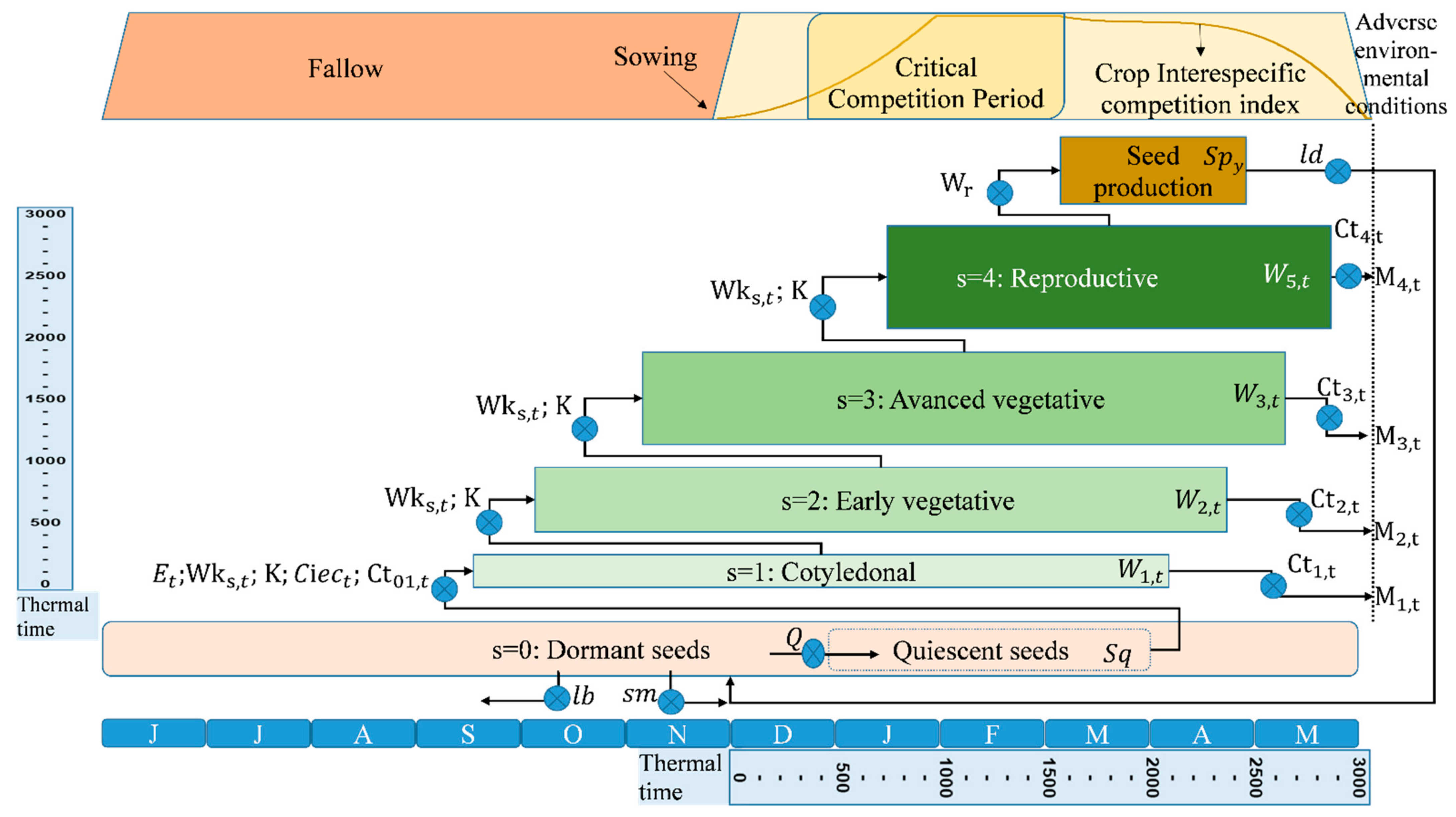
This model uses bioecological and agronomic information as inputs, such as daily weather records, weed population dynamics data, weed-management tactics (chemical, mechanical, and cultural methods), and crops’ ecophysiological requirements. Typical results are the daily values of weed population dynamics, crop-growth/development dynamics, and the resulting weed–crop competitive interactions. At the end of each crop season, both bioecological and agronomic outputs are obtained (i.e., seed production, economic gross margin, environmental impact, etc.).

In this work, the model from Molinari et al. (2020) [5] was extended to improve the economic and environmental evaluation of weed-management strategies. Specifically, the calculation of the present value of money was included to improve economic comparisons in multi-year simulations. Additionally, the quantification of the environmental impact was extended with the T index, which represents the soil-erosion risk associated with mechanical weed control [6]. The P index [6] was also added to quantify the environmental impact of pesticides, complementing the EIQ index calculations [7].

In this study, the described model is applied to the agricultural system Euphorbia davidii Subils in competition with soybean in the center of the Buenos Aires province (Argentina). Euphorbia davidii belongs to the Euphorbiaceae Juss. family, represented by species of economic value and others considered to be weeds [8,9,10]. Four species have been found in Argentina that behave as important weeds in summer crops (Euphorbia serpens, Euphorbia heterophylla, Euphorbia dentata, and Euphorbia davidii), sharing many common characteristics, which complicates their easy identification, and, therefore, the design of effective management strategies for each one [11]. Euphorbia davidii has been reported as an invasive species in multiple regions of Europe [12]. In the agrosystems of the central part of the Buenos Aires province, E. davidii is considered a highly competitive weed that is difficult to control. In general, there is a close relationship between phenological stage, dose, and control efficacy [13,14]. According to [14], under semi-controlled conditions, yield losses of 35–45% are observed in soybean crops at weed densities higher than 100 individuals.m⁻². Likewise, in the study area, field experiments indicate yield losses of 30% at 100 individuals.m⁻², with significant losses observed from 8–10 individuals.m⁻² onwards [15].

It is hypothesized that a previously developed model [5] can be adapted to the agricultural system composed of Euphorbia davidii Subils in competition with soybean in the center of the Buenos Aires province, in order to support decision making for integrated weed management.

The objectives of this article are: (i) to extend the model proposed in [5] with additional detail in the economic and environmental impact modules; (ii) to evaluate the model when applied to the soybean/E. davidii agricultural system in the central-southern region of the Buenos Aires province; (iii) to generate annual and multiannual scenarios comparing different management strategies; and (iv) to evaluate the model’s advantages/weaknesses for its future adaptation to other agrosystems.

2. Materials and Methods

2.1. General Description

The adopted modelling methodology was reported previously in [5]. Certain processes were modified in the present contribution for a better adaptation to the E. davidii/soybean system for the central region of the Buenos Aires province, Argentina. The main features of the model, together with the introduced modifications, are described in detail below.

2.2. Diagram, Variables and Parameters of the Model

In Figure 1, a general diagram of the proposed simulation model, considering an annual cycle of weed–crop competition is presented.

Model sets and variables are summarized in

Table 1. Model sets and variables.

Sets/Variables	Description	Units
t	Julian day	Julian day.
y	Year	Year
s	Weed phenological stage	-
Ws,t	Accumulated weed density in s, t	(i.m−2)
Is,t	Incoming cohorts of individuals in s, t	(i.m−2)
Os,t	Outcoming cohorts of individuals of s, t	(i.m−2)
Ms,t	Accumulation of individuals eliminated by control methods plus those affected by thermal/hydric stress in s, t	(i.m−2)
Sq	Quiescent (non-dormant) seeds	(s.m−2)
Spy	Total weed seed production in y	(s.m−2)
Et	Emerged individuals in t	(i.m−2)
Wks,t	Weighted weed density between s and ns in t	-
Ciect	Crop competition index in t	-
r	Reproductive cohorts’ group	-
Wr	Accumulated weed density in r	(i.m−2)
Yld	Expected crop yield (proportion of weed-free yield)	-
WC	Weed–crop interspecific competition	-
Cts,t	Weed mortality rate due to control in s, t	-
MCs,t	Individuals eliminated by control methods in s, t	-
M_stresss,t	Individuals affected by thermal/hydric stress in s, t	(i.m−2)
Cr01,t	Weed mortality rate over a pre-seedling stage by residual herbicides in s, t	-

. The demographic parameters of E. davidii and soybean crop are detailed in

Table 2. Euphorbia davidii parameters. TT = thermal time. (℮) = estimated, only used in multiannual simulations. EK = expert knowledge.

Parameter	Description		Value	Units	Reference
ns	Number of phenological stages (s)		4	-	[14,16]
Tb	Base temperature for TT accumulation		8	°C	[11]
Th1	TT required for a cohort for transition from	s = 1 to 2	192	°Cd	[14,16]
Th2		s = 2 to 3	300
Th3		s = 3 to 4	700
Qy	Seed proportion produced in year y that are quiescent in year 0	y = −1	0.5	-	℮
		y = −2	0.2
		y = −3	0.15
		y = −4	0.10
		y = −5	0.05
sm	Seed bank annual mortality rate		0.0732	-	℮
ld	Seed loss rate at natural dispersal		0.77	-	℮
lb	Seed loss rate by biotic factors during the first fallow (predation, mortality)		0.2075	-	℮
K	Agrosystem’s carrying capacity		150	i.m−2	[14,16]
f1	Competition factor for stage	s = 1	0.1	-	[14,16]
f2		s = 2	0.5
f3		s = 3	0.75
f4		s = 4	1
nr	Number of simulated groups of reproductive cohorts		1	-	[14,16]
ta	Day of adverse environmental conditions (stress), ta(T°)		−1 < T° > 40	°C	EK
mstress1	Mortality rate due to adverse environmental conditions	s = 1	1	-	EK
mstress2		s = 2	0.6
mstress3		s = 3	0.4
mstress4		s = 4	0

and

Table 3. Soybean crop parameters (sowing time, standard, and delay). EK = expert knowledge. * = adapted from.

Parameter	Description		Value		Units	Reference
			Standard	Delay
G1	Accumulated TT at the time of equation changing		1325	780	°Cd	DSSAT *
G2	Accumulated TT for physiological maturity		2750	1900	°Cd	DSSAT *
CCP	Critical competition period		450–1730	450–1120	°Cd	DSSAT *
Sft	Susceptibility of crop	between 0 ≤ t < CCP	1		-	EK
Sft		during the CCP	5
Sft		between CCP and physiological maturity	1
LAIhc	Value of LAI representing a highly competition situation for different distances between rows	35 cm	0.9	0.9	-	EK and [17]
		52.5 cm	1.5	-	-
		70 cm	2.2	-	-
Myl	Maximum yield loss proportion (high interspecific competition)		0.6		-	Cal. y Valid.
a	Crop-derived constant		0		-	Cal. Y Valid.
k	Weed competitiveness constant		0.1		-	Cal. Y Valid.
GY	Expected grain yield		3000		Kg.ha−1	EK

, respectively.

2.3. Meteorological Data

Weed and crop population dynamics were simulated using daily based meteorological data. Two open access sources were used: the Olavarría Meteorological Station (National Meteorological Service of Argentina) (36°53′20″ S; 60°13′40″ W) and the Regional Centre of Agrometeorology (Faculty of Agronomy, National University of the Center of Buenos Aires Province, Argentina UNCPBA) (http://www1.faa.unicen.edu.ar/centro/centroreg.php, accessed on 21 September 2022, in Spanish) (36°47′00″ S; 59°51′00″ W).

2.4. Euphorbia Davidii Field Emergence

A model was fitted based on meteorological data to predict daily field emergence throughout the agronomic season. For this purpose, the meteorological and field emergence data (36°58′4.30″ S; 60°11′45.35″ W) reported in [14,16] were used. The methodology proposed in [18] was used to model field emergence, with a good fitting level between the observed and predicted data (RMSE = 0.05).

2.5. Population Dynamics

Weed population dynamics were simulated through daily cohorts (Figure 1). The individuals of each cohort went through four phenological stages within the life cycle: s = 1: cotyledon; s = 2: early vegetative (2–4 true leaves); s = 3: advanced vegetative (6 true leaves to branching); s = 4: reproductive (flowering and fruiting). Each cohort required the accumulation of a given thermal time (TT) in order to pass from one phenological stage to the next. When moving from one phenological stage to the next, each cohort was affected by mortality and competition rates (Ct_s,t, Cr_01,t, mstress_s), as detailed in [5]. Reference values for these parameters are reported in Table 2.

2.6. Intraspecific Competition

The competitive effect of weed individuals on each other was calculated using the mortality rate in [5]. In the present work, this was replaced with the following function:

$${\mathrm{I}}_{\mathrm{s},\mathrm{t}}=\max \left\{{\mathrm{O}}_{\mathrm{s}-1,\mathrm{t}} \left[1-\left(\frac{{\mathrm{Wk}}_{\mathrm{s},\mathrm{t}}}{\mathrm{K}}\right)\right];0\right\} \forall \mathrm{t},\forall \mathrm{s}$$

(1)

where I_s,t represents the incoming cohorts at stage s on day t; O_s-1,t stands for the outgoing cohorts from stage s − 1 on day t; Wk_s,t is the weighted weed density from stage s to ns on day t; and K is the agrosystem carrying capacity. The ratio between Wk_s,t and K determines the mortality of the cohorts entering stage s. The maximum function establishes that when Wk_s,t is above K, the incoming individuals are zero. This uncommon situation only occurs when the first cohorts are very abundant.

2.7. Weed Population Mortality

Euphorbia davidii mortality was divided according to their origin: anthropogenic and abiotic. Abiotic mortality was modelled in the current version as a reduction due to extreme temperature events:

$$\left\{\begin{array}{cc}\hfill \mathrm{M}\_{\mathrm{stress}}_{\mathrm{s},\mathrm{t}}={\mathrm{W}}_{\mathrm{s},\mathrm{t}} {\mathrm{mstress}}_{\mathrm{s}}, & |\mathrm{If} {\mathrm{Tmin}}_{\mathrm{t}}<-1 \mathrm{or} {\mathrm{Tmax}}_{\mathrm{t}}>40\hfill \\ \hfill \mathrm{M}\_{\mathrm{stress}}_{\mathrm{s},\mathrm{t}}=0, & |\mathrm{otherwise}\hfill \end{array}\right\} \forall \mathrm{s},\forall \mathrm{t}$$

(2)

where M_stress_s,t is the number of individuals affected by adverse environmental conditions at stage s and day t; mstresss is the mortality rate due to extreme temperatures at stage s; and Tmin_t and Tmax_t are the minimum and maximum temperatures at day t (Table 2).

Weed mortality related to control actions is described in [5]. Control methods are specified in

Table 4. Control methods and toxicity values, Tmam, Tins, and Tf, used for the P index calculation and tillage tool impact values, Timp, for the T index calculation.

Abbreviation		Control Methods
		G3	G + Imz	G + Flp	Dplg	Dhrw
Description		Non-selective (G3)	Non-selective + residual (G + imz)	Non-selective mixture (G + flp)	Disc plough (Dplg)	Disc harrow (Dhrw)
Control method/herbicides, formulation and rate		Glyphosate SL (40.5%): 3 L.ha−1	Glyphosate (66.2%): 2 L.ha−1 + imazethapyr (10%): SL, 1 L.ha−1	Glyphosate (66,2%): 2 L.ha−1 + fluroxypyr CE (48%): 0.4 L.ha−1	Disc plough	Disc harrow
Residual time span [days]		-	30	-	-	-
Residual effect (Cr01,t)		-	1	-	-	-
Mortality rate of control for	s = 1 (Ct1)	0.99	0.99	0.99	0.99	0.99
	s = 2 (Ct2)	0.85	0.85	0.85	0.99	0.99
	s = 3 (Ct3)	0.80	0.80	0.80	0.99	0.99
	s = 4 (Ct4)	0.30	0.29	0.30	0.99	0.99
Herbicide + application cost [USD.ha−1]		52	40	46	40	37
Field EIQ [EIQ.ha−1]		18.63	22.25	19.45	0	0
p index	Tmam	0.607	0.02	0.76	0	0
	Tins	12.15	1	14.31	0	0
	Tf	12.15	0.294	26.67	0	0
T index		Timp	0	0	0	0.86	0.74

References: [13,19,20,21,22].

, together with the corresponding associated economic and environmental parameters.

2.8. Environmental Impact

The environmental impact module quantified the impact of different management strategies through three indexes: the Environmental Impact Quotient (EIQ) [7], pesticide index (P) [6,23], and tillage index (T) [6]. The EIQ and P indexes quantified the environmental impact associated with chemical control, and the T index quantified the environmental impact due to soil erosion caused by tillage tools.

For each active ingredient, EIQ parameters were obtained from an updated source, [24] and the field EIQ value per hectare was calculated according to [7] (Table 4). Tmam, Tins, Tf, and Timp were calculated from toxicity values obtained from [25].

2.9. Economic Evaluation

The economic module calculated the gross margin (GM) and net present value (NPV). The GM directly compares the most relevant costs and incomes, without taking into account the land’s opportunity cost or the rental cost. For multiannual simulations, the NPV is required, as it considers the temporal money value. The NPV was calculated from the GM according to a very well-known methodology [26]. The economic parameters are detailed in

Table 5. Economic parameters.

Parameter Description	Value		Reference
	Standard Density	High Density
Sowing cost (seed + sown + fertilization + inoculant)	164 USD.ha−1	177 USD.ha−1	[19]
Grain sale price	370 USD.tn−1
Harvest cost	72 USD.ha−1
Marketing cost	15% of the gross income
Discount rate	15%		[27]

.

2.10. Weed Seed Production

Seed production was estimated at the end of the weed’s life cycle as a function of the number of individuals that reach the reproductive stage. For its calculation, the function of Equation (3) is used (adapted from [14,16]).

$${\mathrm{Sp}}_{\mathrm{y}}=\left\{\begin{array}{cc}\hfill \left(-80.37 \log {\mathrm{W}}_{\mathrm{r}}+220.6\right) \log {\mathrm{W}}_{\mathrm{r}}, & |\mathrm{If} \left({\mathrm{W}}_{\mathrm{r}}\le 18\right)\hfill \\ \hfill 4870 \log {\mathrm{W}}_{\mathrm{r}}-3952, & |\mathrm{If} \left({\mathrm{W}}_{\mathrm{r}}>18\right)\hfill \end{array}\right\} \forall \mathrm{r},\forall \mathrm{y}$$

(3)

where Sp_y is the seed production in year y, and W_r is the individual density in the reproductive cohort r.

3. Calibration and Validation

To properly estimate the expected crop yield (Yld), parameters a and k of Equation (4) were tuned for the system under study [3].

$$\mathrm{Yld}=\frac{\mathrm{Cs}+\mathrm{a}}{\mathrm{Cs}} \left[\frac{\mathrm{Ca}}{\left(\mathrm{a}+\mathrm{Ca}+\left(\mathrm{k} \mathrm{WC}\right)\right)} \mathrm{Myl}+\left(1-\mathrm{Myl}\right)\right]$$

(4)

where Yld is the expected crop yield (as a proportion of the weed-free yield), Cs is the standard crop density, a is a crop-dependent constant, Ca is the actual crop sowing density, k is a constant reflecting the weed competitiveness of the crop, WC is the sum of the weed competitive effects on the crop at the end of the season, and Myl is the maximum yield loss proportion at high interspecific competition.

In this contribution, parameters a and k were calculated by solving a parameter estimation problem using experimental data reported in [15,28,29,30]. Field trials were conducted in the Azul district (36°47′00″ S; 59°51′00″ W), Buenos Aires province, Argentina. Different cultural management strategies (i.e., soybean crop varieties, sowing dates, row spacing, and sowing densities), as well as herbicides and mechanical control, were included. Field trials reported in [15,29,30] were repeated over two crop seasons, while those reported in [29] were carried out for a single crop season.

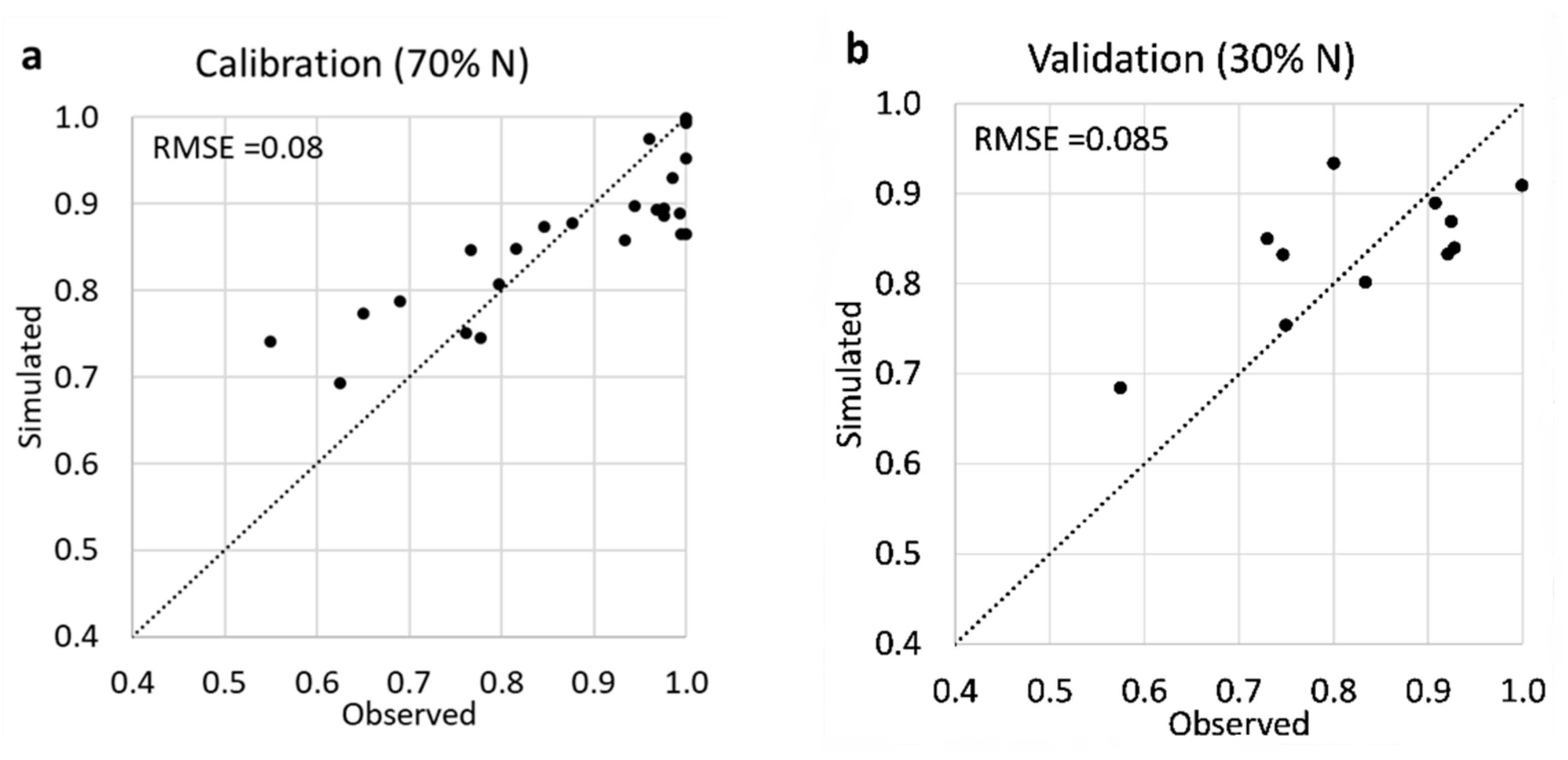
The available experimental data (N = 37) were divided 70/30% for calibration and validation, respectively (randomly selected). Parameters, a and k, that minimize the root-mean-square Error (RMSE) between the observed and simulated Yld were obtained using the solver add-on in the MS Excel spreadsheet version 2013 (Microsoft Corporation, Redmond, WA, USA) (a = 0 and k = 0.1, RMSE = 0.08) (Figure 2a).

Next, we simulated the validation dataset and compared it with the observed data, obtaining an RMSE = 0.085 as shown in Figure 2b.

4. Results

Several case studies were generated to analyze the performance of the model for the soybean/E. davidii agrosystem. Several management strategies and their impact on the crop and the weed were simulated. Two annual case studies with two comparative sub-cases in each one (i.e., operational horizon) and one multiannual case study (i.e., tactical horizon) were presented.

4.1. Annual Case Studies (Operational Horizon)

Table 6. Input parameters for cases I and II (and sub-cases A and B). Case I, mechanical and cultural management. Case II, chemical control and cultural management.

Description	Case I		Case II		Units
	Sub-Case A	Sub-Case B	Sub-Case A	Sub-Case B
Quiescent seeds (weed)	1400		1400		s.m−2
Emergence source	Observed		Observed		-
Sowing density	42	30	42	30	Pl.m−2
Distance between rows	35		35	70	cm
Sowing date	11/7/13	12/20/13	11/7/13		m/d/y
Date and control type during fallow	11/6/13	12/19/13	10/28/13 Non-selective + residual (G + imz)		m/d/y -
	Disc plough

details the cases and sub-cases analyzed.

4.1.1. Case I. Mechanical and Cultural Management

For case I, two simulations were presented using only cultural and mechanical management methods, therefore excluding chemical control actions. Specifically, a mechanical control during fallow, combined with cultural management techniques, such as different sowing densities, sowing dates, and inter-row spacing of the soybean crop, were represented. The management methods used for each sub-case are detailed in Table 6. The simulation results are shown in

Table 7. Output simulation variables corresponding to the annual cases.

Variable		Case I		Case II		Units
		Sub-Case A	Sub-Case B	Sub-Case A	Sub-Case B
Environmental impact	EIQ	0		22.25		-
	P index	0		0.002		-
	T index	0.31		0		-
Total E. davidii seed production		5388	598	2237	3667	s.m−2
E. davidii/soybean interspecific competition		230.06	7.97	35.58	65.41	-
Expected crop yield		78	98	95	89	%
Gross Margin		455	654	651	607	USD.ha−1

and Figure 3.

In sub-case A, a mechanical intervention was simulated the day before the crop sowing date at the corresponding density and inter-row spacing. This approach is clearly insufficient to suppress most of the new E. davidii seedlings that compete with the crop, reaching about 80 individuals.m⁻² at the reproductive stage (Figure 3a).

In sub-case B (Figure 3b), the main cultural management method introduced aimed to delay the soybean sowing date to avoid the E. davidii emergence peak that affected sub-case A. The mechanical fallow was carried out the day before sowing, controlling all emerged individuals up to that date.

The final simulation results (Table 7) suggested two contrasting sub-cases, with better results for the management strategy of sub-case B. The advantages of sub-case B are clearly shown in the economic indicator (Table 7). Both sub-cases had exactly the same values of environmental impact indicators as they differ only in cultural management methods. A penalty in the T index was obtained by tillage. The EIQ and P indexes were null as no pesticides were applied.

4.1.2. Case II. Chemical Control and Cultural Management

Case II simulated the application of an herbicide mixture (glyphosate + imazethapyr) 10 days before soybean sowing. This case was divided into two sub-cases (A and B) with different cultural management alternatives regarding sowing density and inter-row spacing. This case mainly aimed to illustrate both the effect of cultural methods and the impact of residual chemical control treatments on weed population dynamics (Figure 4).

As in the previous case, there were two large emergence events in mid-October. These flows were controlled with the herbicide mixture applied at the end of October, with the residual effect of imazethapyr extending into November (Figure 4).

The final simulation results favored sub-case A, both in agronomic and economic aspects, due to cultural management methods (Table 7). Both sub-cases had exactly the same environmental impact indicator values as they only differed in cultural methods. An impact due to herbicide application (EIQ and P index) was shown, while the T index was null.

4.2. Case III. Multiannual Case Study (Tactical Horizon)

The performance of the model within a tactical (medium-term) horizon was evaluated. Several parameters had to be estimated in order to generate multiannual scenarios due to the lack of specific information on the seed-bank dynamics of E. davidii. Seed-bank parameters include longevity, dormancy, mortality, seed loss, and seed-dispersal rates.

In this case, a weed-management strategy which adopts, each year, the same cultural measures, but with variations in the control methods adopted each agronomic season, was presented. A 5-year horizon was investigated (1996 to 2001).

Table 8. Input parameters for the multiannual simulation case.

Description	Input Parameters					Units
Simulation time period	5					years
Quiescent seeds (weed)	2800	-	-	-	-	s.m−2
Emergence source	Simulated					-
Sowing density	42					Pl.m−2
Distance between rows	35					cm
Sowing date	11/10/1996	11/10/1997	11/10/1998	11/9/1999	11/9/2000	m/d/y
Date and pre-sowing control type	11/9/1996	11/9/1997	11/9/1998	11/8/1999	11/8/2000	m/d/y
	Disc harrow (Dhrw)	Non-selective + residual (G + imz)	Disc plough (Dplg)	Non-selective (G3)	Non-selective mixture (G + flp)	-

and

Table 9. Output simulation variables corresponding to the multiannual case.

Variables		1996	1997	1998	1999	2000	Units
Environmental impact	EIQ	0	22.25	0	18.62	27.33	-
	P index	0	0.002	0	0.075	0.093	-
	T index	0.28	0	0.31	0	0	-
Total E. davidii seed production		2271	3196	523	1040	1371	s.m−2
E. davidii—soybean interspecific competition		51	80	8	18	26	-
Expected crop yield		93	90	98	97	96	%
Gross margin		596	564	644	620	616	USD.ha−1
Net present value		3579					USD.ha−1

show the corresponding input parameters and output variables for the multiannual simulation. Simulation results are presented in Figure 5.

Figure 5 shows the population dynamics of E. davidii simulated for a 5-year period starting with a very high infestation (2800 quiescent seeds.m⁻²) and the combined effect of cultural, chemical, and mechanical control tactics.

Cultural management was based on crop sowing at a high density and a reduced row spacing, causing a fast canopy inter-rowing which results in an early competition with the weed at the expense of a higher sowing cost (Table 8 and Figure 5).

Controls were carried out during fallow and varied between different types of chemical options and tillage (Table 8).

Analyzing the annual dynamics, we observed that the first weed flush was controlled by pre-sowing interventions with some individuals escaping control and further competing with the crop (Figure 5). The second emergence flush also generated competition to some extent, while the third flush (between December and January) was effectively suppressed by interspecific soybean competition, which was reinforced by cultural measures.

For the multiannual scenario, the applied weed-management measures significantly reduced the initial infestation. High competition and seed production occurred during the 1996 and 1997 seasons with a sensible reduction in subsequent years. In the first two seasons, the expected crop yield was partially affected, although without a considerable yield loss (Table 9). In the remaining three years, the crop averaged 97% of its potential yield.

The environmental indexes show differences according to the type of control used each season. In particular, in 2000, the non-selective herbicide mixture (G + flp) produced a negative environmental impact (Table 9). The gross margin remained between 564 and 644 USD.ha⁻¹, and a 3579 USD.ha⁻¹ present value.

5. Conclusions

In this contribution, a very detailed population-based model [5] was extended by improving the multi-year economic calculations, and by adding new indexes to estimate pesticides and soil-erosion impact, to better compare and evaluate alternative weed-management strategies.

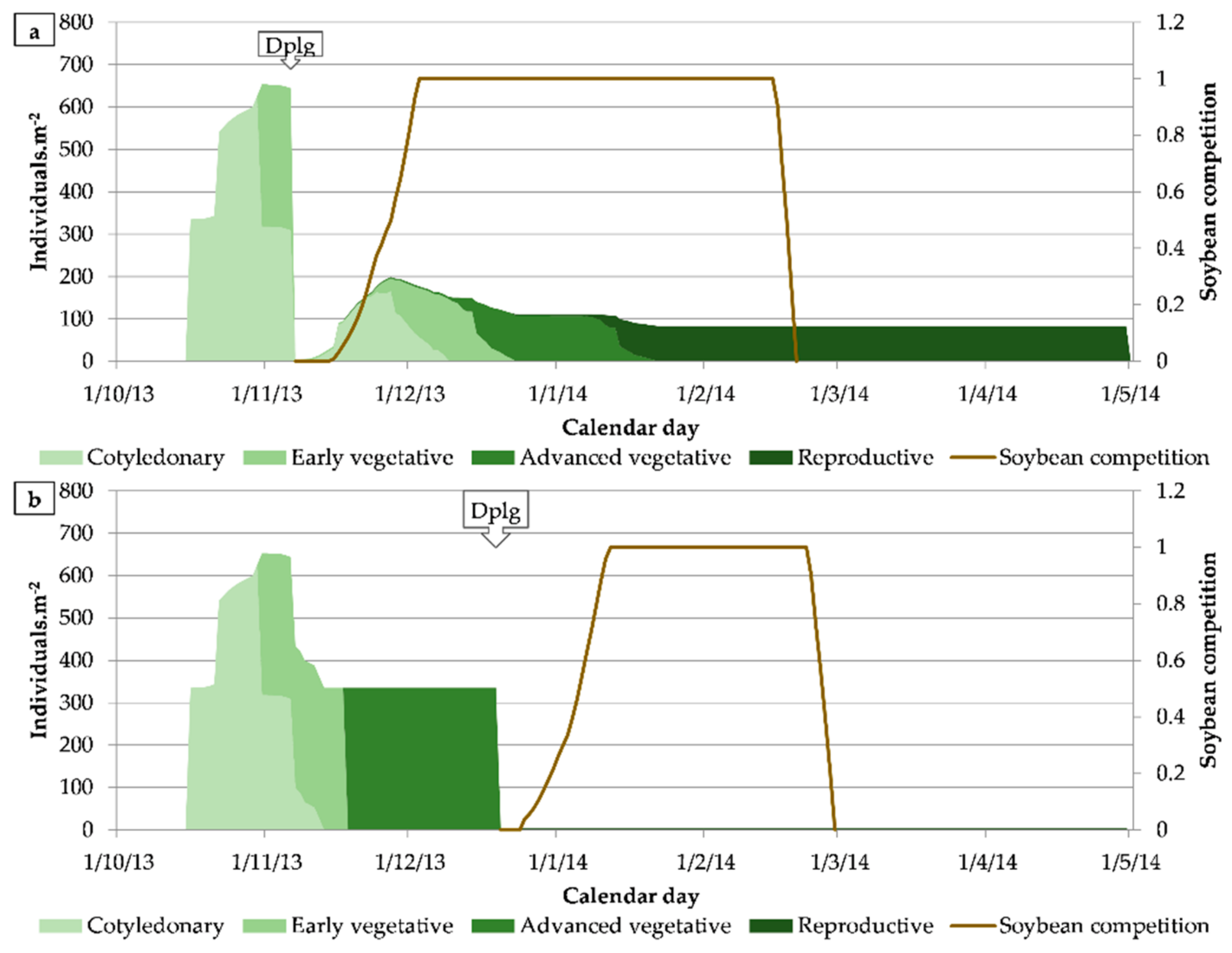
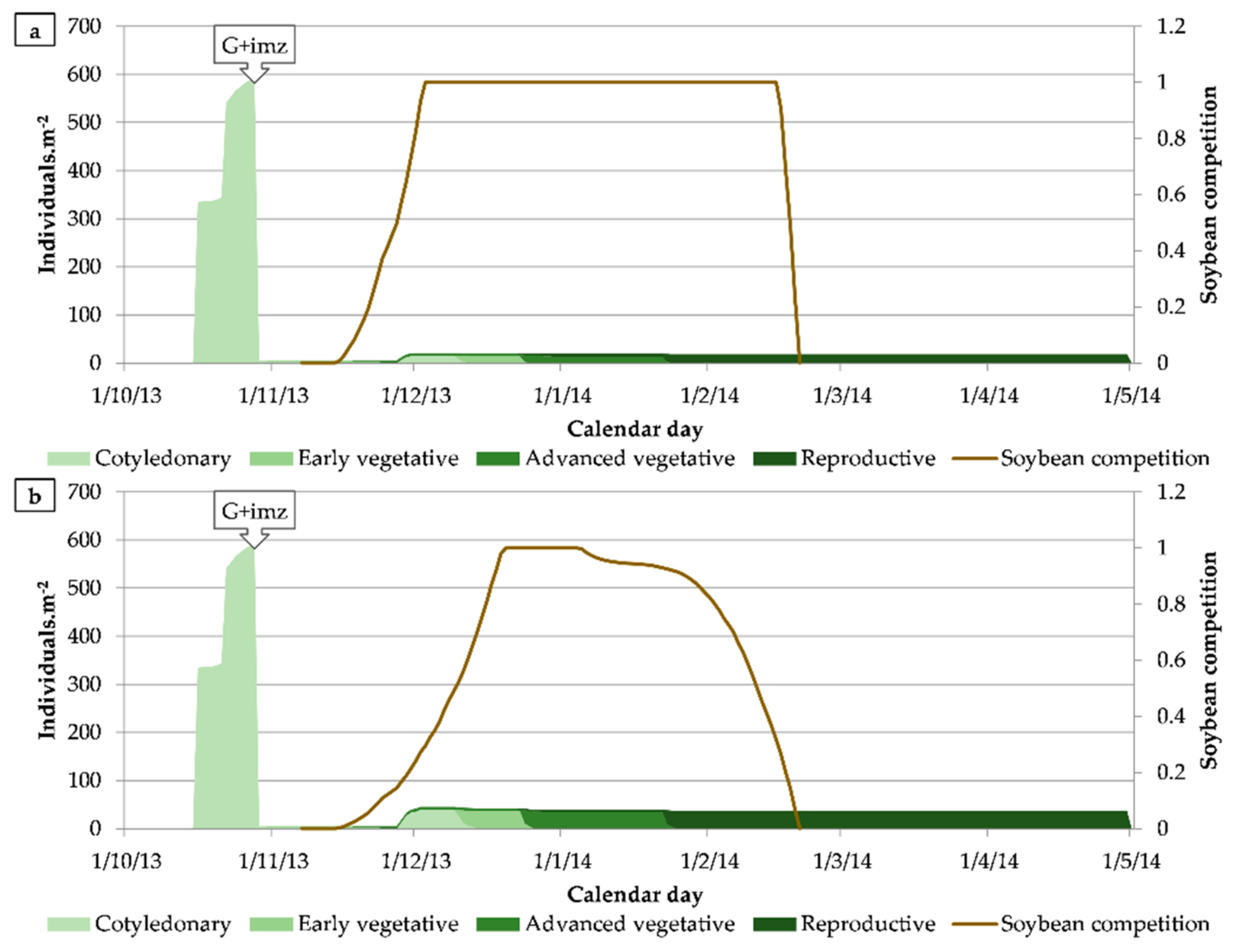
Following this, the model was adapted to a typical soybean/Euphorbia davidii agrosystem for the center of the Buenos Aires province, Argentina. Annual and multiannual case studies were simulated to analyze crop–weed interactions under different cultural measures and control actions (chemical and mechanical).

In general, the simulated results showed that, under high infestation conditions, it was necessary to combine: (i) an estimation of weed-emergence flowrates; (ii) the adoption of cultural management methods, such as delayed sowing times, higher sowing densities, and narrower distances between rows; (iii) chemical control methods, especially the use of a mixture of non-selective and residual herbicides, in combination with mechanical methods due to their high control rate of E. davidii at advanced development stages. By making such combinations, satisfactory agronomic outcomes could be obtained without having a high impact on gross margin and externalities due to chemical and/or mechanical actions.

While the proposed approach seems to provide a balance in terms of biological, agronomic, economic, and environmental details of the complex agrosystem under study, many improvements for future adaptations can be outlined. For example, it is known that E. davidii can coexist with several other weeds. The modelling of a multispecies agrosystem requires a great deal of specific information. Another extension that should be incorporated in future versions of the model is weed-resistance quantification, which should be considered in long-period studies for strategic and integrated weed management.

References

1. Andrew, I.K.S.; Storkey, J.; Sparkes, D.L. A Review of the Potential for Competitive Cereal Cultivars as a Tool in Integrated Weed Management. Weed Res. 2015, 55, 239–248. [Google Scholar] [CrossRef] [PubMed]
2. Scursoni, J.A.; Vera, A.C.D.; Oreja, F.H.; Kruk, B.C.; De La Fuente, E.B. Weed Management Practices in Argentina Crops. Weed Technol. 2019, 33, 459–463. [Google Scholar] [CrossRef]
3. Pannell, D.J.; Stewart, V.; Bennett, A.; Monjardino, M.; Schmidt, C.; Powles, S.B. RIM: A Bioeconomic Model for Integrated Weed Management of Lolium Rigidum in Western Australia. Agric. Syst. 2004, 79, 305–325. [Google Scholar] [CrossRef]
4. Bagavathiannan, M.V.; Beckie, H.J.; Chantre, G.R.; Gonzalez-Andujar, J.L.; Leon, R.G.; Neve, P.; Poggio, S.L.; Schutte, B.J.; Somerville, G.J.; Werle, R.; et al. Simulation Models on the Ecology and Management of Arableweeds: Structure, Quantitative Insights, and Applications. Agronomy 2020, 10, 161. [Google Scholar] [CrossRef]
5. Molinari, F.A.; Blanco, A.M.; Vigna, M.R.; Chantre, G.R. Towards an Integrated Weed Management Decision Support System: A Simulation Model for Weed-Crop Competition and Control. Comput. Electron. Agric. 2020, 175, 105597. [Google Scholar] [CrossRef]
6. Ferraro, D.O.; Ghersa, C.M.; Sznaider, G.A. Evaluation of Environmental Impact Indicators Using Fuzzy Logic to Assess the Mixed Cropping Systems of the Inland Pampa, Argentina. Agric. Ecosyst. Environ. 2003, 96, 1–18. [Google Scholar] [CrossRef]
7. Kovach, J.; Petzoldt, C.; Degni, J.; Tette, J. A Method to Measure the Environmental Impact of Pesticides. N. Y. Food Life Sci. Bull. 1992, 139, 1–8. [Google Scholar]
8. Tanveer, A.; Khaliq, A.; Javaid, M.M.; Chaudhry, M.N.; Awan, I. Implications of Weeds of Genus Euphorbia for Crop Production: A Review. Planta Daninha 2013, 31, 723–731. [Google Scholar] [CrossRef]
9. Palma-Bautista, C.; Rojano-Delgado, A.M.; Vázquez-García, J.G.; Yanniccari, M.; Prado, R. De Resistance to Fomesafen, Imazamox and Glyphosate in Euphorbia Heterophylla from Brazil. Agronomy 2020, 10, 1573. [Google Scholar] [CrossRef]
10. Cavalcante, N.B.; Diego da Conceição Santos, A.; Guedes da Silva Almeida, J.R. The Genus Jatropha (Euphorbiaceae): A Review on Secondary Chemical Metabolites and Biological Aspects. Chem. Biol. Interact. 2020, 318, 108976. [Google Scholar] [CrossRef] [PubMed]
11. Marchessi, J.E.; Subils, R.; Scaramuzzino, R.L.; Crosta, H.N.; Eseiza, M.F.; Saint André, H.M.; Juan, V.F. Presencia de Euphorbia Davidii Subils (Euphorbiaceae) En La Provincia de Buenos Aires: Morfología y Anatomía de La Especie Presence of Euphorbia Davidii Subils (Euphorbiaceae) in Buenos Aires Province: Morphology and Anatomy. Kurtziana 2011, 36, 45–53. [Google Scholar]
12. Barina, Z.; Shevera, M.; Sîrbu, C.; Pinke, G. Current Distribution and Spreading of Euphorbia Davidii (E. Dentata Agg.) in Europe. Cent. Eur. J. Biol. 2013, 8, 87–95. [Google Scholar] [CrossRef]
13. Istilart, C.; Yanniccari, M.; Gigón, R.; Lucrecia, M.; Horacio, F. Control de Lecherón (Euphorbia Davidii) En Post-Emergencia de Maíz Resistente a Glifosato. Ser. Inf. Técnicos 2014, 3, 101–103. [Google Scholar]
14. Núñez Fré, F.R.; Juan, V.F.; Saint-André, H.M.; Chantre, G.R. Demographic and Phenological Studies on David’s Spurge (Euphorbia Davidii) in the Central Area of Buenos Aires Province, Argentina. Planta Daninha 2018, 36, 1–14. [Google Scholar] [CrossRef]
15. Juan, V.F.; Saint-Andre, H.; Fernandez, R.R. Competencia de Lecheron (Euphorbia Dentata) En Soja. Planta Daninha 2003, 21, 175–180. [Google Scholar] [CrossRef]
16. Nuñez Fré, F.R. Manejo de Euphorbia Davidii Subils: Dinámica Poblacional, Control Químico y Evaluación de Sensibilidad a Glifosato; Universidad Nacional del Sur: Bahía Blanca, Buenos Aires, Argentina, 2019. [Google Scholar]
17. Meira, S.; Rodríguez Baide, J.M.; Confalone, A.; Fatecha Fois, D.A.; Fernandes, J.M.; González Pérez, O.; Van den Berg, M. Modelación Del Cultivo de Soja En Latinoamérica Estado Del Arte y Base de Datos Para Parametrización; EU: Maastricht, The Netherlands, 2019. [Google Scholar]
18. Chantre, G.R.; Vigna, M.R.; Renzi, J.P.; Blanco, A.M. A Flexible and Practical Approach for Real-Time Weed Emergence Prediction Based on Artificial Neural Networks. Biosyst. Eng. 2018, 170, 51–60. [Google Scholar] [CrossRef]
19. Revista Margenes Agropecuarios. Buenos Aires, Argentina. 2022, pp. 34–57, 1 April 2022. Available online: https://www.margenes.com/ (accessed on 27 August 2022).
20. Juan, V.F.; Marchessi, J.E.; Núñez Fré, F. Control de Lecheron (Euphorbia Dentata) Con Glifosato. Planta Daninha 2006, 24, 347–352. [Google Scholar] [CrossRef]
21. Núñez Fré, F.; Juan, V.; Saint André, H.; Fernández, R. Evaluación de Herbicidas Residuales Complementando a Glifosato Para El Control de Euphorbia Davidii En Barbechos. In Proceedings of the XXI Congreso Latinoamericano de Malezas, de la Asociación Latinoamericana de Malezas (ALAM). I Congreso argentino de Malezas, de la Asociación Civil Argentina de Ciencia de las Malezas (ASACIM), Buenos Aires, Argentina, 10 September 2015; p. 90. [Google Scholar]
22. Núñez Fré, F.R.; Juan, V.F.; Yanniccari, M.; Saint-André, H.M.; Fernandez, R.R. Comparison of Sensitivity to Glyphosate of Euphorbia Davidii Populations. Planta Daninha 2017, 36, 1–9. [Google Scholar] [CrossRef]
23. Ferraro, D.O. PRORIPEST. Available online: http://proripest.malezas.agro.uba.ar/inicio.php (accessed on 9 May 2022).
24. Eshenaur, B.; Grant, J.; Kovach, J.; Petzoldt, C.; Degni, J.; Tette, J. Environmental Impact Quotient: A Method to Measure the Environmental Impact of Pesticides. Available online: www.nysipm.cornell.edu/publications/EIQ (accessed on 13 December 2019).
25. University of Hertfordshire PPDB: Pesticide Properties DataBase. Available online: https://sitem.herts.ac.uk/ (accessed on 30 April 2022).
26. Gaspars-Wieloch, H. Role of Scenario Planning and Probabilities in Economic Decision Problems–Literature Review and New Conclusions. In Proceedings of the 6th International Scientific Conference Contemporary Issues in Business, Management and Economics Engineering, Vilnius, Lithuania, 9–10 May 2019. [Google Scholar] [CrossRef]
27. Bolsa de Cereales de Buenos Aires. Available online: https://www.bolsadecereales.com/margenes-agricolas (accessed on 31 May 2022).
28. Juan, V.; Saint-André, H.M. Control of Lecheron (Euphorbia Dentata) in Soybean with Imazethapyr Applied at Defferent Developmental Stages. Actas XIII Congr. Latinoam. Malezas. 1997, 2, pp. 128–132. Available online: https://www.researchgate.net/publication/277954783_Control_of_Lecheron_Euphorbia_dentata_in_soybean_with_imazethapyr_applied_at_defferent_developmental_stages?channel=doi&linkId=55772a7508ae753637538d38&showFulltext=true (accessed on 27 August 2022). [CrossRef]
29. Juan, V.F.; Saint-André, H.M.; Fernández, R.R.; Videla, M.; Bazzano, J. Control de Euphorbia Dentata En Soja Con Herbicidas Post-Emergentes. Rev. Bras. Herbic. 2000, 1, 147. [Google Scholar] [CrossRef]
30. Juan, V.F.; Saint-André, H.M.; Fernández, R.R.; Bazzano, J.; Videla, M. Control de Euphorbia Dentata Con Diferentes Formulaciones de Glifosato En Soja Transgenica Resistente a Glifosato. Rev. Bras. Herbic. 2002, 3, 29. [Google Scholar] [CrossRef] [Green Version]
Figure 1. General diagram showing the key elements of the simulation model, displaying how E. davidii competes with soybean over a crop season (see Table 1, Table 2 and Table 3 for description of variables and parameters). On the left, a thermal time scale used to guide the weed life-cycle development is shown. A thermal and chronological time scale for crop-growth development is displayed at the base of the diagram. At the top, the fallow and crop cycle are schematized, including the most important indexes. The weed life cycle is represented in a simple way by the most representative stages (Ws,t): dormant and quiescent seeds in the seed bank; cotyledonal (cotyledons); early vegetative (2 to 4 true leaves); advanced vegetative (6 true leaves to branching); and reproductive (flowering and fruiting).
Agronomy 12 02369 g001
Figure 2. Calibration (a) and validation (b) of the expected yield function Yld.
Agronomy 12 02369 g002
Figure 3. Euphorbia davidii population dynamics. In different shades of green are the relative composition of each phenological stage, starting from a large seedbank (1400 quiescent seeds.m−2). Arrows indicate control methods and application dates. The effect of mechanical control was simulated with a disc plough. The soybean crop is represented by the crop-competition index. (a) Sub-case A and (b) sub-case B.
Agronomy 12 02369 g003
Figure 4. Euphorbia davidii population dynamics. In different shades of green are the relative composition of each phenological stage, starting from a large seedbank (1400 quiescent seeds.m−2). Arrows indicate control methods and application dates. The chemical control effect was simulated using a mixture of non-selective and residual herbicides G + imz (Glyphosate 66.2%, 2 L. ha−1 and imazethapyr LS 10%, 1 L. ha−1). The soybean crop is represented by the crop-competition index. (a) Sub-case A and (b) sub-case B.
Agronomy 12 02369 g004
Figure 5. Euphorbia davidii population dynamics. In different shades of green are the relative composition of each phenological stage, starting from a very high initial seed infestation (2800 quiescent seeds.m−2). Arrows indicate different control methods and application dates. The effect of the following control methods were simulated: Dhrw (Disc harrow); G + imz (Glyphosate (66.2%): 2 L.ha−1 + imazethapyr (10%): SL, 1 L.ha−1); Dplg (Disc plough); G3 (Glyphosate SL (40.5%): 3 L.ha−1) and G + flp (Glyphosate (66.2%): 2 L.ha−1 + fluroxypyr CE (48%): 0.4 L.ha−1). The soybean crop is represented by the crop-competition index. The Y-axis was scaled to 450 individuals.m−2 to improve results visualization.
Agronomy 12 02369 g005