Abstract
This study presents a tracer technique based on the fluorescent properties of quinine to help on the visualization of shallow flows and allow a quantitative measurement of overland flow velocities. Laboratory experiments were conducted to compare the traditional dye tracer and thermal tracer techniques with this novel fluorescent (quinine) tracer by injecting a quinine solution and the other tracers into shallow flowing surface water. The leading-edge tracer velocities, estimated using videos of the experiments with the quinine tracer were compared with the velocities obtained by using thermograms and real imaging videos of the dye tracers. The results show that the quinine tracer can be used to estimate both overland and rill flow velocities, since measurements are similar to those resulting from using other commonly used tracers. The main advantage of using the quinine tracer is the higher visibility of the injected tracer under ultraviolet A (UVA) light for low luminosity conditions. In addition, smaller amounts of quinine tracer are needed than for dye tracers, which lead to smaller disturbances in the flow. It requires a simple experimental setup and is non-toxic to the environment.
1. Introduction
Surface water flow velocities and discharges are essential to understand the hydraulic dynamics of shallow flows, namely in irrigated land and urban environments (e.g., [1]). Moreover, the accurate estimation of flow velocities is important to understand natural phenomena such as runoff, overland flow, rill development, erosion and infiltration and for modelling surface runoff, and sediment and solute transport (e.g., [1,2]). In recent years there have been many studies conducted in the field and in the laboratory, which have contributed to a better understanding of surface flow processes (e.g., wave front movements, tracers’ leading-edge movements, surface velocity fields). One of the important approaches for measuring and modelling surface flow processes in the field is to monitor water movements by flow tracing techniques (e.g., [3,4,5,6]).
Artificial tracers are substances that are introduced into the hydrologic system to obtain information on the processes under study. The success of tracing techniques is highly dependent on the selection of the proper tracer as its application is limited both in time and space (e.g., [3,4,7]). This requires a good understanding of the behaviour of the tracer in different environmental conditions. Typical fields of application are: detection of hydrological connectivity, flow paths, determination of flow velocities, hydrodynamic dispersion, runoff separation, resident time, simulation of contaminant transport and discharge measurement applying the dilution methods (e.g., [3]).
For the specific study of surface runoff, most commonly used approaches use colour (dye) tracers (e.g., [5,8]), fluorescence dyes (e.g., [3,6,9]), drifting particles (e.g., [10,11]), salt tracers and electrolytes (e.g., [8,12,13]), or radioactive isotopes (e.g., [14]), which have been used as traditional tracking tools by scientists over the years.
Additionally, a number of recent studies have been conducted on thermal tracer techniques such as the infrared thermographic approach for shallow overland flow estimation in laboratory and field experiments (e.g., [5,6,8,13,15,16]). This technique was used to measure surface flow velocity by tracking the leading-edge of a heated tracer solution instead of using an optical camera or the naked eye, which is usually associated with dye tracing techniques.
Fluorescent dye tracing methods are also widely used and are probably the most important artificial tracers [3,4,10,11]). They are used, for example, to identify connections between groundwater supply points (e.g., sinkholes, karst windows, etc.), discharge points (e.g., springs and wells), and to estimate the solute-transport characteristics (e.g., travel time of the leading edge of the dye, peak dye concentration, persistence of the dye plume at the discharge point, trajectory tracking, etc.) (e.g., [3,17]). According to these authors, fluorescent tracers have less limitations than non-fluorescent detectors, in particular, their low toxicity levels compared with other tracer substances. Several non-toxic and non-carcinogenic dyes, such as uranine, rhodamines, eosine, pyranine, and naphthionate are available (e.g., [3,18]).
In this experimental study, quinine was used as a novel fluorescent tracer for estimating leading-edge velocities aiming to obtain overland flow and rill flow velocities. The main goals of this study were: (i) to test this new fluorescent tracer’s capability, which, in combination with ultraviolet A (UVA) light, supports measuring the velocity of shallow flows, (ii) to compare the results with traditional dye tracing and infrared thermographic techniques for various discharges and bare soil surface morphological conditions, and (iii) to test in which conditions the use of this novel tracer is an advantage.
2. Materials and Methods
2.1. Laboratory Setups
This study follows others that used soil flumes to study surface hydrological processes (e.g., [19,20,21,22,23,24]). Three slightly different simple laboratory setups were used for the qualitative and quantitative comparison of the fluorescent (quinine) tracer, the thermal tracer, and the dye tracer techniques, for estimating overland flow leading-edge velocities (Figure 1). The experiments were carried out in a 3.0 m long by 0.3 m wide rectangular soil flume, adjusted to a 1% slope, with a surface water supply system installed upstream of the flume. The water supply system comprised a constant head tank and a feeder box, thus allowing the application of a known constant flow over the flume soil surface. A tubular shape ultraviolet lamp UVA (BLB light bulb) was used (Nominal power: 36 W; UVA Irradiance @ 20 cm, 315–400 nm: 350 mW/cm2; Peak emission wavelength: 354 nm).

Figure 1.
Schematic representation of the laboratory setup for: (a) Quinine tracer; (b) Thermal tracer; and (c) Dye tracer measurements.
The constant head tank was filled with tap water from the laboratory supply system (Conductivity: 75.9–150 µS/cm at 20 °C; pH: 6.5–7.3; Turbidity: < 1.1 NTU; O2: 1.0–3.7 mg/L; Total hardness: 21.4–33.3 mg CaCO3/L; [25]), which was also used to prepare the tracers.
2.2. Soil and Surface Morphology
The 0.1 m deep soil layer used in the flume is a sandy loam, which was collected from fluvial deposits from the right bank of the river Mondego, near the vicinity of Coimbra, Portugal (already used in previous studies, e.g., [5,26]). The main physical characteristics of the soil used in the soil flume experiments are: Sand content: 79%; Silt content: 10%; Clay content: 11%; Bulk density: 1100 kg/m3; Soil depth: 62 mm; Colour: brownish.
The soil was saturated, and a small amount of hydraulic cement (Portland cement) was applied superficially, whenever needed, to guarantee the preservation of the soil surface microrelief throughout the experiments, i.e., without suffering any type of erosion. Then, the soil surface was left to dry (more than 1 week) until it gained a consistency that assured the preservation of the soil surface characteristics.
Following this procedure, three surface morphologies were tested (Figure 2). The eroded plane surface was created by run-on applied by a feeder box installed at the upstream end of the soil flume.
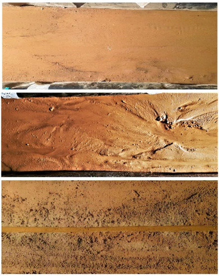
Figure 2.
Photographs of the scanned surface area (see Figure 1) with the flat plane surface (top), the eroded plane surface (middle) and the artificial rill (bottom). The longitudinal dimension of each photograph is 0.5 m.
2.3. Tracers
The following tracers were used: (1) dye tracer; (2) quinine fluorescent tracer; and (3) thermal tracer. The three techniques were tested with the same conditions (same soil surface morphology, discharge, flow depths and velocities). The flow was kept in steady state.
2.3.1. Dye Tracer
For the dye tracer solution, a red food colouring (Ingredients: carmoisine dye (E122), ponceau dye 4R (E124), yellow dye (E104) and acetic acid (E260)) was used by diluting it in tap water with a concentration of 20 mL/L.
2.3.2. Quinine Fluorescent Tracer
Quinine is known as a bitter alkaloid that is extracted from the bark of the cinchona tree and has been used in medical treatments (e.g., [27,28]). Quinine can also be applied as a bitter flavouring agent in soft drinks such as tonic water. Tonic water includes approximately 80 mg/L of quinine [29,30].
In this set of experiments, the following quinine was used: monohydrochloride dihydrate 99% (ACROS Organics™). Quinine monohydrochloride dihydrate 99% has no ecotoxicological effects in the environment and is not likely mobile in soil due to its low water solubility [31]. Following preliminary tests, a concentration of 80 mg/L was used since its fluorescence was adequate for the proposed use.
2.3.3. Thermal Tracer
For the thermal tracer experiments, water was heated in a kettle to a temperature of approximately 80 °C. In the experiments, the average overland flow temperature was in the range of 18.0–20.0 °C.
2.4. Video Recording Systems
Both infrared video and real image video were used. Thermal videos of the scanned area (Figure 1) were recorded with the FLIR DUO PRO R infrared video camera (Resolution (number of pixels): 336 × 256; Accuracy: +/- 5 °C or 5% of readings in the −25 °C to +135 °C range; Spectral range: 7.5–13.5 μm). Real image videos were recorded with a regular cell-phone Samsung S8 optical camera (Resolution (number of pixels): 4290 × 2800 photographs; 1920 × 1080 video frames). For all the experiments, the cameras were in a fixed position; however, the infrared camera had a different position than the optical camera, in order to catch the same flume’s area. Therefore, the optical and infrared cameras were attached to a metal support structure, respectively, 0.65 m and 1.5 m above the soil surface; the cameras were installed with the sensor parallel to the soil surface.
The infrared video camera detects the invisible infrared energy emitted by the wetted soil surface and water, presenting it as a 2D visual image. The imaging scale of the infrared camera is based on the temperature emissivity coefficients of the materials. Since the water and wetted soil emissivity coefficients are very similar (maximum of 15%), for the working spectral range of the infrared camera (7.5–13.5 μm) the associated errors can be ignored.
To improve the visualization of the dye tracer in the real image videos, the flume was positioned to minimize the reflections of light off the surface of the water flow. In order to visualize the fluorescent tracer, an ultraviolet (UVA) lamp was installed beside the flume and the background was covered with black plastic to avoid light reflection and obtain high quality imagery.
2.5. Laboratory Procedure and Image Processing
Since the objective of this study was to compare the quinine (fluorescent) with the dye and thermal tracer techniques, no attempt was made to estimate the mean flow velocity for the cross-sectional area (across the flume). Many studies have focused on determining the velocity of dye tracers by tracking the leading-edge of the tracer (e.g., [9]), which is related to the surface velocity of flow.
The leading-edge velocity was measured from the video frames and used as the variable for comparison between tracers, as illustrated in Figure 3. Therefore, no correction factors were applied, as suggested by many authors when mean flow velocities are to be estimated (e.g., [5,9,32,33]). Since the flume had a constant width, it was straightforward to estimate the distances travelled by the leading-edge in a certain time-span within two frames (Figure 3). In addition, no correction was done to the field of view since all tracers were subjected to the same perspective.
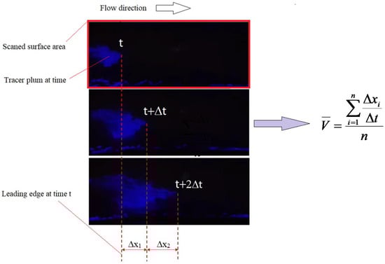
Figure 3.
Method of estimating mean leading-edge tracer surface velocity (here illustrated for the quinine tracer tracking). The blue intermittent lines at the bottom of the scanning area are reflections captured by the camera and should be disregarded.
Three sets of experiments were performed: (i) on a flat plane surface under overland flow that covered approximately uniformly the entire soil surface (sheet flow); (ii) over an eroded surface, created by water erosion, with overland flow meandering through the natural relief of the eroded soil with varying flow depths according to the micro-relief; (iii) inside an artificial rill with the whole flow contained within the rill (Figure 2).
Flow velocity was measured for different flow discharge rates and volumes of tracer, at the downstream end of the flume (Figure 1). Discharge applied to the upstream end of the soil flume surface through run-on from the feeder tank was controlled manually from the water supply system using a valve until steady state flow was achieved.
Once discharge became stable, the velocity measurements were undertaken at the measuring section (video scanned area) with the optical and infrared video cameras. The movement of the tracer along the scanned area was recorded in separate videos, for each tracer type and settings. Three replicates were conducted for each flow discharge rate and volume of tracer injected (5, 7.5 and 10 mL). The scanned area was established 1.0 m downslope of the feeder tank, with a length of 0.5 m over the flume width.
The tracers (quinine, dye and thermal) were applied with the help of a syringe at approximately 0.2 m upslope of the scanned area, to minimize the interference of the injection volume in the velocity measurements in the scanned section. The syringe had a maximum capacity of 10 mL to allow testing with different volumes.
Frames were visualized and analysed one by one with MATLAB image processing toolbox. In the case of quinine, the aim was to identify the brightness intensity of the fluorescent tracer. All videos and images were converted to grayscale; therefore, the brightness intensity range for the fluorescent tracer varied from 0 to 255. For the thermal videos, FLIR Tools® (software to import, edit, and analyse thermal images) was used.
3. Results and Discussion
To illustrate what is captured in the different videos, Figure 4 shows frames of the scanned areas recorded by the cameras. These illustrate the differences between the fluorescent (quinine), dye, and thermal tracer videos. In addition, the differences between the flat and eroded surfaces, and the artificial rill become clear, since the concentrated rill flow has well-defined boundaries.
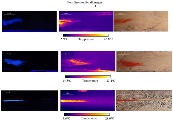
Figure 4.
Comparison between imaging of the quinine tracer under ultraviolet light (left), the thermal tracer snapshots (centre), and the dye tracer (right), for the flat plane (top), eroded (middle), and artificial rill (bottom) surfaces. Scales are indicated on the images.
An example of the chronological sequence of images of the scanned area for the different tracers can be seen in Figure 5. The aim of this figure is solely to illustrate the difference of the movement, over time, of the three tracers used in this study. The thermal tracer leading-edge movement is initially better shaped, particularly when a threshold temperature is used (e.g., [5]); however, it leaves a thermal mark that takes some time to fade away since the soil surface warms up as the heated tracer passes over it. This happens because of the very small flow depth (few millimetres). It should be noted that from time t = 4 s onwards the leading-edge is not visible any more. The quinine tracer leading-edge movement is better defined and better shaped, and does not leave any mark or residue in the measuring section (video scanned area), as suspended quinine moves with the flow.
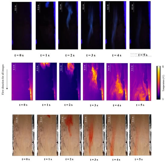
Figure 5.
Chronological sequence of snapshots for overland flow tests, with a time lapse of 1 s, for: quinine tracer (top), thermal tracer (middle), and dye tracer (bottom) measurements. Snapshots of the scanned surface area are from the flat plane surface (see Figure 2). The blue intermittent marks (top) on the sides of the scanning area are reflections captured by the camera, and should be disregarded.
Table 1, Table 2 and Table 3 summarize the data for all studied cases. Leading-edge velocities are presented (average and standard deviation for three replicates). Mean velocity and standard deviation (S.D.) of tracers’ leading-edge for the three applied tracer volumes are also shown.

Table 1.
Plane surface flow test results for thermal, dye and quinine fluorescent tracer leading-edge velocities, for different discharges and tracer volumes. The data are for three replicates of each combination. Notation “-“ means no data.
Table 2.
Eroded surface flow test results for thermal, dye and quinine fluorescent tracer leading-edge velocities, for different discharges and tracer volumes. The data are for three replicates of each combination. Notation “-“ means no data.
Table 3.
Rill flow test results for thermal, dye and quinine fluorescent tracer leading-edge velocities, for different discharges and tracer volumes. The data are for three replicates of each combination.
The combined analyses of Figure 6 and results presented in Table 1, Table 2 and Table 3 show that the injected tracer leading-edge velocities, estimated by all techniques, are similar for all flow discharges and volumes of tracer used. Larger volumes of tracer lead to slightly higher flow velocities; this is clearly more relevant for small discharges, where the influence of the volume of injected tracer is more noticeable.
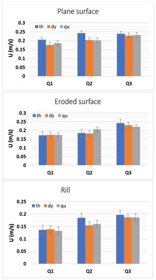
Figure 6.
Comparison of injected tracer leading-edge velocities U measured for the three tracers (total of 81 tests for each tracer), for the plane surface, eroded surface and rill flows. Mean and standard deviation are presented for each flow discharge Q (detailed data in Table 1, Table 2 and Table 3).
The three techniques studied yielded very similar results, as can be seen in Figure 7; the comparison between the velocities measured using the dye and fluorescent tracers showed a good correlation, with a coefficient of determination for a linear regression (R2) of 0.99, for all the tested surfaces. In addition, the comparison between the velocities measured using the thermal tracer and the other tracers shows that the thermal tracer overestimates the velocities when compared to the other two techniques. Nonetheless, the R2 is approximately 0.99 for all cases. The regression equations and R2 related to Figure 7 are presented in Table 4.
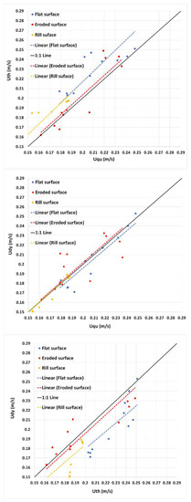
Figure 7.
Comparison between velocities measured by the quinine (Uqu), dye (Udy) and thermal (Uth) tracer techniques, for the flat plane, eroded surface and artificial straight rill. Line 1:1 and linear regression lines are also plotted. Note that the axes are not at the origin (0,0).
Table 4.
The regression equations and coefficient of determination (R2) of graphs in Figure 7.
The brightness intensity of the fluorescent tracer at each time step, with Δt = 1 s, was plotted (Figure 8) along the length of the flume (scanned area) and compared with the temperature variation of the thermal tracer for the same time step. During this time lapse, the maximum fluorescent intensity decreases, due to diffusion and mass transport, from a value of 65 to 42, which is still highly visible. On the other hand, the temperature drops from 27 °C to 22 °C, which is close to the temperature of the soil and water, making it difficult to track the exact point of the hot tracer leading-edge. Hence it can be concluded that for the same time step, the fluorescent tracer seems to remain more visible than the thermal tracer. In addition, the thermal tracer leaves a thermal mark spread over the surface that takes some time to fade out, due to the heating of the soil surface as the thermal tracer passes over it.
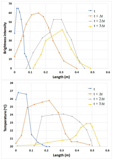
Figure 8.
Brightness of the fluorescent quinine tracer (top) and temperature of the thermal tracer (bottom) over time (t, t + Δt, t + 2Δt, t + 3Δt), along the flume’s length (scanned area). Comparison between the two graphs shows that the decay of temperature in the thermogram is stronger than the reduction of brightness intensity in the quinine tracer. These examples are from tracer movements over the plane surface (Q = 113.63 mL/s, Vtr = 7.5 mL).
For the quinine solution tracer, Figure 9 shows in detail the tracer movement over the scanned area. The brightness intensity contour plots (Figure 9a) allow one to visualize the movement of the tracer over the soil surface and to extract data that enables one to evaluate how brightness intensity evolves along time (Figure 9b). The well-defined contour plots show that quinine solution is capable of maintaining its visibility under UVA lights, and so, maintain its tracing features. The decay in brightness is directly related to the concentration of quinine in the flow, which results from the dispersion patterns caused by the shallow-flow hydrodynamics.
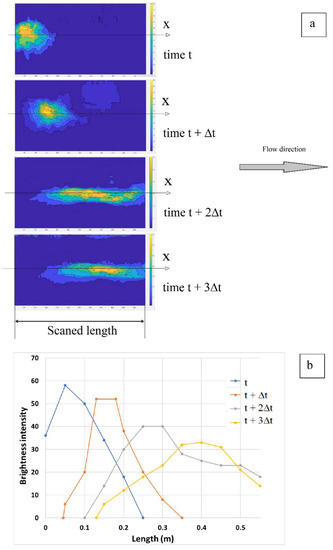
Figure 9.
Quinine tracer movement over the scanned area for one run over the plane surface (Q = 113.63 mL/s, Vtr = 10 mL): (a) Brightness intensity contour plots and (b) Brightness intensity along the flume’s length x (scanned area), in time (t, t + Δt, t + 2Δt, t + 3Δt).
4. Conclusions
The results show that quinine tracer under ultraviolet light can be used to estimate overland flow velocities, for both sheet flows and rill flows. Leading-edge velocity estimates are nearly identical to those recorded for dye tracers, a technique widely used to estimate shallow flow velocities, and similar to measurements carried out using the thermal tracers, a more recent technique. This demonstrates the viability of using quinine as a tracer for surface hydrology studies.
The main advantages of using fluorescent quinine as a tracer are: (i) Higher visibility of the injected tracer compared with dye tracing; (ii) It requires a simple experimental setup (e.g., UVA lamp which is inexpensive and easy to get, a camera and water with quinine); (iii) Smaller amounts of quinine tracer are needed than for dye tracers, which leads to smaller disturbances in the flow; (iv) High visibility of the injected tracer with low luminosity conditions (e.g., field measurements in dark conditions, at night, twilight, shielded environments such as under heavy vegetation or close conduits); (v) The technique is less expensive than thermal tracers because it does not need a thermographic camera; (vi) It is non-toxic to the environment, due to the very low concentration needed to produce high fluorescence (around 80 mg/L, a concentration that is used in tonic water for human consumption, for example). The fluorescent tracer should not be used under sunny conditions, however, since the advantage of the fluorescence disappears; other types of tracers are therefore recommended.
More work is needed to evaluate the capabilities of the quinine tracer technique when applied in different urban and rural surface conditions (e.g., cobblestone pavements, road pavements, arable land, mulch covers). Field protocols must be also designed and prepared, particularly bearing in mind that the fluorescence of quinine tracer depends on the quinine solution concentration and water characteristics. The applicability of this novel tracer to estimate flow velocities in streams and rivers is yet to be established.
Author Contributions
J.L.M.P.d.L., R.M. and J.M.G.P.I. conceived and designed the experiments; S.Z. and R.G.J. performed the experiments; S.Z. and J.L.M.P.d.L. analysed the data; J.L.M.P.d.L. and S.Z. wrote the paper; J.L.M.P.d.L., J.M.G.P.I. and M.I.P.d.L. revised the manuscript. All authors have read and agreed to the published version of the manuscript.
Funding
This research was funded by the Portuguese Foundation for Science and Technology (FCT), through projects ASHMOB (CENTRO-01-0145-FEDER-029351), MUSSELFLOW (PTDC/BIA-EVL/29199/2017), MEDWATERICE (PRIMA/0006/2018), and through the strategic project UIDB/04292/2020 granted to MARE—Marine and Environmental Sciences Centre, University of Coimbra, Coimbra, Portugal. The second author was granted a PhD fellowship from FCT (Ref. 2020.07183.BD).
Acknowledgments
The authors acknowledge the Laboratory of Hydraulics, Water Resources and Environment of the Department of Civil Engineering of the University of Coimbra, where the experimental work was conducted.
Conflicts of Interest
The authors declare that there are no conflicts of interest.
References
- Singh, V.P. Handbook of Applied Hydrology; McGraw-Hill Education: New York, NY, USA, 2017; 1440p. [Google Scholar]
- Chow, V.T.; Maidment, D.R.; Mays, L.W. Applied Hydrology; McGraw-Hill: New York, NY, USA, 1988. [Google Scholar]
- Leibundgut, C.; Maloszewski, P.; Külls, C. Tracers in Hydrology; Wiley-Blackwell: Hoboken, NJ, USA, 2009. [Google Scholar]
- Tauro, F.; Aureli, M.; Porfiri, M.; Grimaldi, S. Characterization of Buoyant Fluorescent Particles for Field Observations of Water Flows. Sensors 2010, 10, 11512–11529. [Google Scholar] [CrossRef] [Green Version]
- de Lima, J.L.M.P.; Abrantes, J.R.C.B. Using a thermal tracer to estimate overland and rill flow velocities. Earth Surf. Process. Landf. 2014, 30, 1293–1300. [Google Scholar] [CrossRef]
- Mujtaba, B.; de Lima, J.L.M.P. Laboratory testing of a new thermal tracer for infrared-based PTV technique for shallow overland flows. Catena 2018, 169, 69–79. [Google Scholar] [CrossRef]
- Jodeau, M.; Hauet, A.; Paquier, A.; Le Coz, J.; Dramais, G. Application and evaluation of LS-PIV technique for the monitoring of river surface velocities in high flow conditions. Flow Meas. Instrum. 2008, 19, 117–127. [Google Scholar] [CrossRef] [Green Version]
- Abrantes, J.; Moruzzi, R.; Silveira, A.; de Lima, J.L. Comparison of thermal, salt and dye tracing to estimate shallow flow velocities: Novel triple-tracer approach. J. Hydrol. 2018, 557, 362–377. [Google Scholar] [CrossRef] [Green Version]
- Zhang, G.-H.; Luo, R.-T.; Cao, Y.; Shen, R.-C.; Zhang, X. Correction factor to dye-measured flow velocity under varying water and sediment discharges. J. Hydrol. 2010, 389, 205–213. [Google Scholar] [CrossRef]
- Tauro, F.; Grimaldi, S.; Petroselli, A.; Rulli, M.C.; Porfiri, M. Fluorescent particle tracers in surface hydrology: A proof of concept in a semi-natural hillslope. Hydrol. Earth Syst. Sci. 2012, 16, 2973–2983. [Google Scholar] [CrossRef] [Green Version]
- Tauro, F.; Pagano, C.; Porfiri, M.; Grimaldi, S. Tracing of shallow water flows through buoyant fluorescent particles. Flow Meas. Instrum. 2012, 26, 93–101. [Google Scholar] [CrossRef]
- Lei, T.; Chuo, R.; Zhao, J.; Shi, X.; Liu, L. An improved method for shallow water flow velocity measurement with practical electrolyte inputs. J. Hydrol. 2010, 390, 45–56. [Google Scholar] [CrossRef]
- Schuetz, T.; Weiler, M.; Lange, J.; Stoelzle, M. Two-dimensional assessment of solute transport in shallow waters with thermal imaging and heated water. Adv. Water Resour. 2012, 43, 67–75. [Google Scholar] [CrossRef]
- Zhou, J.; Liu, G.; Meng, Y.; Xia, C.; Chen, K.; Chen, Y. Using stable isotopes as tracer to investigate hydrological condition and estimate water residence time in a plain region, Chengdu, China. Sci. Rep. 2021, 11, 2812. [Google Scholar] [CrossRef] [PubMed]
- de Lima, R.L.; Abrantes, J.R.; de Lima, J.L.; de Lima, M.I.P. Using thermal tracers to estimate flow velocities of shallow flows: Laboratory and field experiments. J. Hydrol. Hydromech. 2015, 63, 255–262. [Google Scholar] [CrossRef] [Green Version]
- Abrantes, J.R.; Moruzzi, R.B.; de Lima, J.L.; Silveira, A.; Montenegro, A.A. Combining a thermal tracer with a transport model to estimate shallow flow velocities. Phys. Chem. Earth Parts A B C 2019, 109, 59–69. [Google Scholar] [CrossRef]
- Buzády, A.; Erostyák, J.; Paál, G. Determination of uranine tracer dye from underground water of Mecsek Hill, Hungary. J. Biochem. Biophys. Methods 2006, 69, 207–214. [Google Scholar] [CrossRef]
- Aley, T.; Fletcher, M.W. The water tracer’s cookbook. Mo. Speleol. 1976, 16, 1–32. [Google Scholar]
- Montenegro, A.A.A.; Abrantes, J.R.C.B.; de Lima, J.L.M.P.; Singh, V.P.; Santos, T.E.M. Impact of mulching on soil and water dynamics under intermittent simulated rainfall. Catena 2013, 109, 139–149. [Google Scholar] [CrossRef]
- Abrantes, J.R.C.B.; de Lima, J.L.M.P.; Montenegro, A.A.A. Performance of kinematic modelling of surface runoff for intermittent rainfall on soils covered with mulch. Rev. Bras. Eng. Agrícola E Ambient. 2015, 19, 166–172. [Google Scholar] [CrossRef] [Green Version]
- Abrantes, J.R.C.B.; Prats, S.A.; Jacob, J.K.; de Lima, J.L.M.P. Effectiveness of the application of rice straw mulching strips in reducing runoff and soil loss: Laboratory soil flume experiments under simulated rainfall. Soil Tillage Res. 2018, 180, 238–249. [Google Scholar] [CrossRef]
- Prats, S.A.; Abrantes, J.R.C.B.; Crema, I.P.; Keizer, J.J.; de Lima, J.L.M.P. Runoff and soil erosion mitigation with sieved forest residue mulch strips under controlled laboratory conditions. For. Ecol. Manag. 2017, 396, 102–112. [Google Scholar] [CrossRef]
- de Lima, J.L.M.P.; Isidoro, J.M.G.P.; de Lima, M.I.P.; Singh, V.P. Longitudinal Hillslope Shape Effects on Runoff and Sediment Loss: Laboratory Flume Experiments. J. Environ. Eng. 2018, 144, 04017097. [Google Scholar] [CrossRef]
- de Lima, J.L.M.P.; Santos, L.; Mujtaba, B.; de Lima, M.I.P. Laboratory assessment of the influence of rice straw mulch size on soil loss. Adv. Geosci. 2019, 48, 11–18. [Google Scholar] [CrossRef] [Green Version]
- Águas de Coimbra, Eem. Quality Control of Water Intended for Human Consumption-Municipality of Coimbra-Boavista Supply Area—1st Semester 2020; Technical Report; Águas de Coimbra, Eem: Coimbra, Portugal, 2020. [Google Scholar]
- de Lima, J.L.M.P.; Singh, V.P.; de Lima, M.I.P. The influence of storm movement on water erosion: Storm direction and velocity effects. Catena 2003, 52, 39–56. [Google Scholar] [CrossRef]
- Diener, H.C.; Dethlefsen, U.; Dethlefsen-Gruber, S.; Verbeek, P. Effectiveness of quinine in treating muscle cramps: A double-blind, placebo-controlled, parallel-group, multicentre trial. Int. J. Clin. Pract. 2002, 56, 243–246. [Google Scholar]
- Geto, A.; Amare, M.; Tessema, M.; Admassie, S. Polymer-modified glassy carbon electrode for the electrochemical detection of quinine in human urine and pharmaceutical formulations. Anal. Bioanal. Chem. 2012, 404, 525–530. [Google Scholar] [CrossRef]
- Awasthi, S.; Srivastava, A.; Singla, M. Voltammetric determination of citric acid and quinine hydrochloride using polypyrrole–pentacyanonitrosylferrate/platinum electrode. Synth. Met. 2011, 161, 1707–1712. [Google Scholar] [CrossRef]
- Donovan, J.L.; DeVane, C.L.; Boulton, D.; Dodd, S.; Markowitz, J.S. Dietary levels of quinine in tonic water do not inhibit CYP2D6 in vivo. Food Chem. Toxicol. 2003, 41, 1199–1201. [Google Scholar] [CrossRef]
- Thermo Fisher Scientific. Safety Data Sheet Quinine Monohydrochloride Dihydrate 99%. Available online: https://www.alfa.com/en/msds/?language=EN&subformat=AGHS&sku=H33474 (accessed on 18 February 2021).
- Li, G.; Abrahams, A.D.; Atkinson, J.F. Correction factors in the determination of mean velocity of overland flow. Earth Surf. Process. Landf. 1996, 21, 509–515. [Google Scholar] [CrossRef]
- Dunkerley, D. Estimating the mean speed of laminar overland flow using dye injection-uncertainty on rough surfaces. Earth Surf. Process. Landf. 2001, 26, 363–374. [Google Scholar] [CrossRef]
Publisher’s Note: MDPI stays neutral with regard to jurisdictional claims in published maps and institutional affiliations. |
© 2021 by the authors. Licensee MDPI, Basel, Switzerland. This article is an open access article distributed under the terms and conditions of the Creative Commons Attribution (CC BY) license (https://creativecommons.org/licenses/by/4.0/).