Spatial Distribution and Development of Sequential Sampling Plans for Diaphorina citri Kuwayama (Hemiptera: Liviidae)

Abstract

Vector control in huanglongbing management has been conducted on a calendar basis resulting in high production costs. We addressed this issue and proposed a sequential sampling plan to support decision making for intervention against Diaphorina citri Kuwayama, which is involved in the transmission of the bacteria Candidatus Liberibacter asiaticus, associated with such lethal disease. We analyzed 3,264,660 records from samples gathered from the Mexican trapping program for the monitoring of D. citri; it included weekly inspection of 86,004 yellow sticky traps distributed in the country. Spatial distribution of the insect, estimation of a common k (kc), and sequential sampling plans based on Sequential Probability Ratio Test (SPRT) were determined. Taylor’s power law coefficients were ≥1 indicating aggregation in the spatial distribution of the insect. Common k ranged from 0.0183 to 0.2253 and varied independently of geographic zone or citrus species. We obtained 18 sequential sampling plans, one for each state. In the Average Sample Number (ASN) function, the minimal number of samples to make a decision ranged from 17 to 65. In the Operational Characteristic (OC) function, probabilities for a correct intervention at the threshold of 0.2 D. citri adults/trap in most cases were above 80%. In a field evaluation, the application of sampling plans yielded savings obtained by reduction in the number of interventions for insect control.

1. Introduction

Huanglongbing (HLB) is a catastrophic disease of cultivated Citrus trees (Rutaceae) [1,2,3]. Presently, there are 66 countries affected in the world, with only the Mediterranean and West Asian citrus producing areas as well as that of Australia and New Zealand, remaining free of the disease [4]. This malady is associated with three forms of a fastidious, phloem limited, and Gram negative α-proteobacterium: Candidatus Liberibacter africanus, Ca. L. americanus, and Ca. L. asiaticus (CLas) [5], with the latter being widely distributed and affecting most of the main major citrus producers worldwide: China, Brazil, India, Mexico, and USA. [3,4,6,7]. Characteristically, CLas is transmitted by the Asian citrus psyllid (ACP) Diaphorina citri Kuwayama (Hemiptera: Liviidae) [1,5,8,9,10]. ACP adults that developed on infected trees were positive for CLas at a rate of 68%, while those that developed on healthy plants were positive at a rate of only 5% [11,12]. For transmission, the bacterium must be acquired during the nymphal stage [9,10,11,12,13]. When the ACP acquires the bacteria as an adult, the rate of acquisition is low and the time for inoculation is long, both of which result in low infection rates [11]. Individual bacteriliferous ACP adults can transmit CLas at a rate of 4–10%, while groups of 200 adults transmitted the bacterium at a rate of 88% [11].

Management of HLB in the affected countries has been based on a three-pronged approach, which includes identification and elimination of infected trees, use of new plants that are certified to have been produced under protective structures, and vector control [3,4,6,7,14]. Li et al. [15] indicate that the use of broad-spectrum insecticides constitutes the only cost-effective strategy for ACP control. Intensive use of chemical control has been performed to eliminate the insect in diverse countries. The use of different numbers of sprays during the year has been evaluated [16,17,18,19] and in Florida citrus growers have used up to 12 sprays or more in the case of young trees [14,20]. In China and Brazil, the number of sprays has a range from 18 [21] up to one/week/all year around (52 in total) [22]. This approach is economically unsustainable [14,23], environmentally unviable, socially questionable, and largely unsuccessful [14,20,23,24] and it is clear that new tools need to be developed and incorporated into the management of ACP [14].

Integrated pest management is used today in many systems as an alternative to calendar-based insecticide applications [18,20,23]. To reinforce this approach, the use of thresholds has been introduced [20,23,25], which were neglected in the HLB management because of the perceived high risk of bacteria transmission [3]. Thus, an important tool to consider in this case is sequential sampling, which incorporates the use of thresholds to aid in decision making. In sequential sampling, unlike classical sampling, the number of samples required is variable instead of fixed and the number and timing of sampling depends on the results obtained at each stage of the procedure [26,27,28,29]. One major advantage of the technique is that the sample size is reduced, in some cases to only 40–50% of the number of samples that would be required in a classical sampling plan. In addition, after each sample is evaluated, there is a decision-making process [27,28,29,30,31,32]. In sequential sampling three possibilities are tested: (1) The null hypothesis is not rejected (no intervention is required); (2) rejection of the null hypothesis (intervention is required); and (3) uncertainty (the decision is to take another sample) [27,28,33]. Sampling can be stopped as soon as enough information has been collected to make the decision for intervention [27,29]. The use of sequential sampling results in pest control being performed only when it is required, yielding a reduced number of interventions in comparison when insecticide sprays are made in a calendar basis [27,33]. The objective of the current study was to generate and test a sequential sampling protocol for D. citri, with the goal of basing management decision on a threshold, which would, in turn, reduce the economic and environmental costs associated with intensive use of insecticide sprays. The generated sampling plan integrates the spatial distribution of the insect and an estimated common k. It is based on the Sequential Probability Ratio Test SPRT [26,30] and observes a nominal threshold with decision lines supported by the Operating Characteristic (OC) and the Average Sample Number (ASN) functions. The generated sequential sampling plan was tested in the field in two commercial citrus groves.

2. Materials and Methods

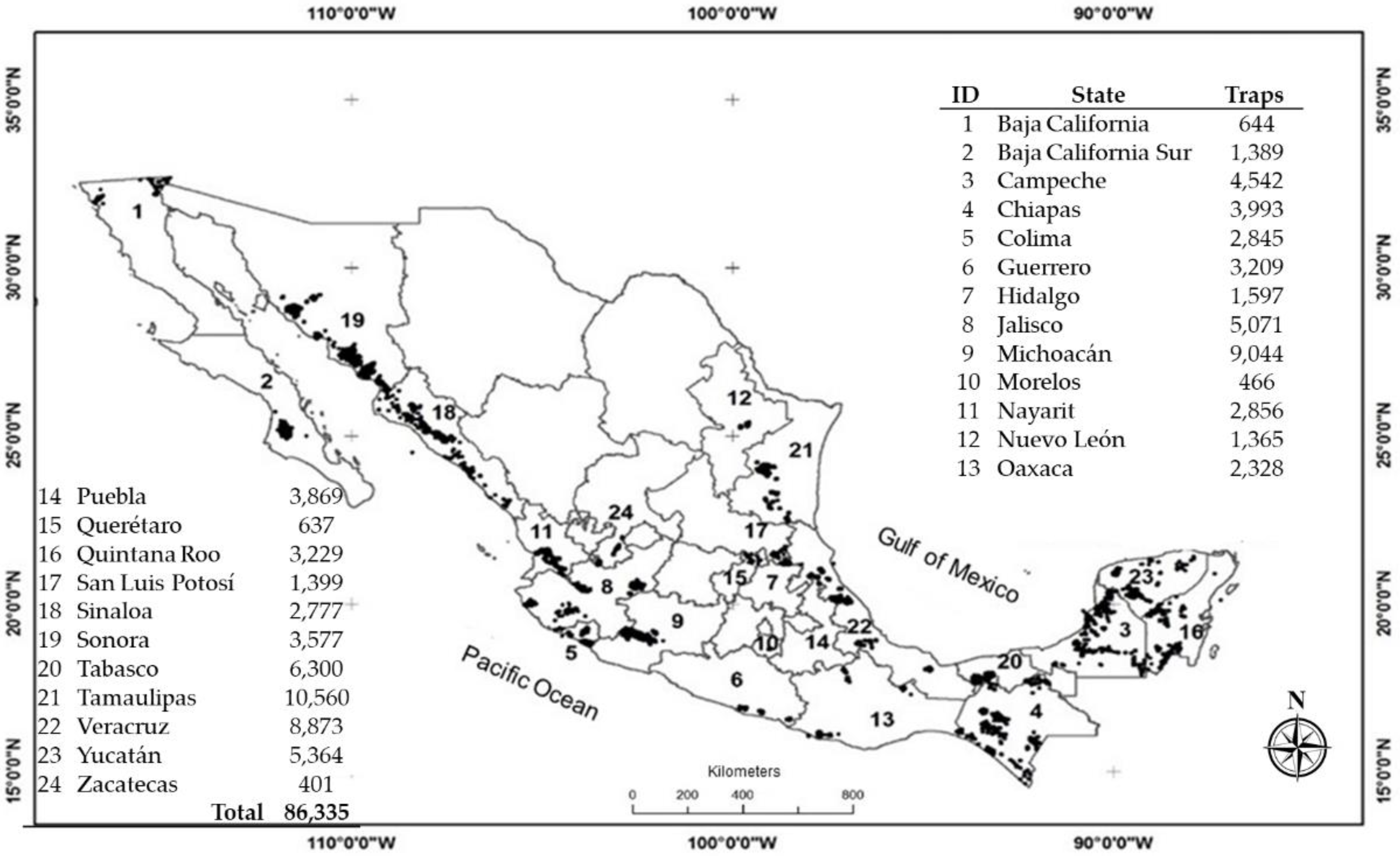
2.1. Data Collection

We used data from the nation-wide trapping program that monitored ACP in the 24 citrus producing states of Mexico during 2015. Yellow sticky traps numbering 86,335 were used to sample the occurrence of ACP adults in Mexican citrus. The traps were made of yellow laminated cardboard that were rectangular shaped and 15 × 22 cm in size. They were installed at 1.5–2 m above the ground on trees located in the perimeter of the grove and in the free frontal side of the tree canopy. They were placed every 200 m in strategically selected groves within the Mexican area-wide management of HLB-ACP named Regional Control Areas (ARCOs), which were established at a national level [34,35]. The geographic distribution of the traps by state is shown in Figure 1.

Each trap had two sticky sides. When first hung, only one side was uncovered and after one week the captured ACP adults were counted and recorded. The trap was then reversed and the other sticky side uncovered. One week later, the captured ACP adults were counted and a new trap was deployed in its place. All traps were replaced every two weeks. With the obtained information, the National Service for Health, Security, and Agri-Food Quality-General Directorate of Plant Health (SENASICA-DGSV) database on the presence of the ACP in the different citrus areas of the country was integrated. These data were analyzed to define aggregation indices and distribution patterns for the pest [36,37,38,39,40]; that information is essential in the generation of a sequential sampling protocol [41]. From the database, the following variables were gathered for the present study: citrus species, municipality, and the number of ACP adults captured per trap/week/tree. Only weeks with traps showing captures of adult specimens were considered for the analysis. The number of traps used in the study varied between weeks and municipalities. The highest number of traps was installed in the state of Tamaulipas with 10,560 traps/week, followed by Michoacán and Veracruz with 9044 and 8873 traps/week, respectively. In total, there were 86,335 deployed traps in the country corresponding to the same number of trees sampled. Once the database was compiled, it sorted 3,264,660 records by municipality, week, and number of captured ACP adults.

2.2. Spatial Distribution of the ACP

An initial step in developing a sampling plan is to determine the spatial distribution of the target insect within the field [37,41,42]. For this, there are several indices of spatial dispersion based mainly on the mean–variance relationship. To confirm the type of dispersion, it is necessary to evaluate more than one index. For the present study, the following aggregation indices were used: relation variance/mean (DI), Taylor’s power law, and the parameter k of the negative binomial, which are described below.

2.2.1. Variance–Mean Relationship (DI)

This relationship is based on the fact that, in a random spatial pattern, the variance $\left(s^2\right)$ of the population density is equal to the mean $\left(m\right)$ [37,43,44]. If this relationship is equal to 1, then the distribution is random; if it is less than 1 it is considered uniform and if it is greater than 1, it is considered aggregated [43]. Thus, the variance/mean ratio is a measure of the deviation from randomness [45,46]. Many studies that describe the use of the variance/mean relationship as a method to analyze aggregation patterns adopt the approach of Greig-Smith [47], who bases the criterion on the degree of departure from the Poisson distribution. A ratio of less than one indicates a regular distribution while a ratio greater than one indicates an aggregated distribution [47].

2.2.2. Taylor’s Power Law

This law describes the relationships between the variance and the sample mean [43] and provides an index of aggregation in terms of ecological parameters [37]. Taylor’s power law relates the variance to the mean density through the following model:

$$s^2 = a{m}^b$$

(1)

where s² is the variance of the density of the sample, $\left(m\right)$ is the mean density of the sample, $\left(a\right)$ an intercept value that is largely a scaling factor related to sample size with no ecological meaning, and ($b$) is the slope, which is an intrinsic property of the species that describes the degree of aggregation of its population in a particular environment and a given time. It is a dispersion index where b < 1, b = 1, or b > 1 indicates a uniform, random, or aggregated dispersion, respectively [43]. These patterns of dispersion are verified by a means of a hypothesis test; for the present case, if D. citri has an aggregate dispersion, the statement of the hypothesis is as follows:

$$H_0:b_1\le 1$$

(2)

$$H_1:b_1>1$$

(3)

which is tested by means of a Student’s t-test.

The Taylor’s power law parameters are obtained through a linear regression of the natural logarithms of the variances on the natural logarithms of the means of each sampled week, adjusting them in a linear regression to obtain the linear equation of the model [43]:

$$\ln s^2 = \ln a+b\ln x.$$

(4)

Precision of b values, according to Downing [48], was estimated by calculating the relationship SE_b/b, where values <0.2 indicate its robustness.

2.2.3. The Negative Binomial Distribution and Its Parameter k

Insect counts in the field are often well fitted by a negative binomial distribution (NBD). The NBD is defined by two parameters which are the arithmetic mean $\left(m\right)$ and the positive exponent k [49]. The parameter k can be used as a measure of aggregation [43] where negative values indicate a regular or uniform distribution, positive values close to zero indicate aggregation, and high values indicate the disposition for a random distribution [37]. For a given insect species, the mean (m) varies under different conditions; however, k remains approximately the same [50].

A fundamental aspect in the definition of a sequential sampling plan is evaluating the possibility of using a common k at the different sampling sites, for which, the procedure described by Bliss and Owen is commonly used [51]. These authors have established two tests to validate its possible use: (1) the ${\chi }^2$ test and (2) the $F$ test. According to the formulas indicated by these authors, an algorithm was developed in R [52], which allowed the calculation and evaluation of a possible kc by the method of moments and by using the method of weighted regression [51] for each of the included citrus producing states.

2.3. Sequential Sampling Plan (SeqSP) Based on Sequential Probability Ratio Test (SPRT)

In the present study, in order to obtain the SeqSP we used the methodology and the nomenclature of variables and parameters presented by Oakland in 1950 [30], which is based on Wald’s Sequential Probability Ratio Test (SPRT) [26]. A fundamental step in the development of a SeqSP is to establish the fitting of a pest density into a frequency distribution. An important parameter in this determination is the mean–variance relationship. Since the variance is significantly greater than the mean densities, a fit to a negative binomial distribution is assumed [31,53]. If the mean density of the pest is fitted by the negative binomial distribution, Oakland [30] presents the procedure to follow to develop a SeqSP, which starts from the definition of the following input variables: a minimum value observed to not apply control $\left(H_0\right)$ indicated as kpo; and another that indicates the average density at which in certain measure of insect population, control must be used, $\left(H_1\right)$, represented as kp1.

In addition to the previous variables, it was necessary to set a level of confidence for the occurrence of type I error (α): apply control when it is not required; or type II error: do not apply control when required (β). Normally, these values can be considered between 0.05 and 0.20. For α and β it is suggested to assign values of 0.1, which is considered an acceptable risk of error [27,28,29,30]. Once the aforementioned parameters had been set:$kpo$, $kp1$, $\alpha$, $\beta$, and kc (common k), the next step was to calculate two auxiliary variables required in the definition of the decision threshold lines and the Average Sample Number function (ASN) described as follows.

$$A=1-\beta /\alpha$$

(5)

$$B=\beta /1-\alpha$$

(6)

In the present study, the assigned value for α and β was 0.10; hence, the probability to have type I or II error was 10%.

The Oakland calculation algorithm begins with the following equations implemented in an Excel spreadsheet.

$$Po=kpo/kc$$

(7)

$$p1=kp1/kc$$

(8)

$$Qo=1+po$$

(9)

$$q1=1+p1$$

(10)

$$kpoqo=\left(kpo\right)\left(Qo\right)$$

(11)

$$kp1q1=\left(kp1\right)\left(q1\right)$$

(12)

The calculation of the acceptance and rejection lines was carried out with the following formulas:

Slope (s) = kc × [ln(q1/q0)]/((ln[((p1 × q0))/((p0 × q1))]))

(13)

Intercept (ho) = ln(B)/((ln[((p1 × q0))/((p0 × q1))]))

(14)

Intercept (h1) = ln(A)/((ln[((p1 × q0))/(p0 × q1)]))

(15)

$$\mathrm{Acceptance}\mathrm{line}=s\left(n\right)+h1;$$

(16)

$$\mathrm{Rejection}\mathrm{line}=s\left(n\right)+h0;$$

(17)

where $n =$ number of samples (traps).

The graph of the operational characteristic curve (OC) was developed with the following expression:

$$L\left(p\right)=Ah-1/Ah-Bh$$

(18)

$$\mathrm{where}:A=1-\beta /\alpha ;$$

(19)

$$B = \beta /1-\alpha ;$$

(20)

$$p=\left[1-{\left(q0/q1\right)}^h\right]/\left\{{\left[\left(p1\times q0\right)/\left(p0\times q1\right)\right]}^h-1\right\}$$

(21)

where h is a dummy variable. For each value of h, a value of $p$ is calculated.

The average number of samples required by the E(n) test is obtained as follows.

$$E\left(n\right)=h1+\left(h0-h1\right)\times L\left(p\right)/\left(kp-s\right)$$

(22)

The calculations for the different p-values generate the curve for the Average Sample Number (ASN). Regarding the average abundance of the number of ACP adults captured per trap per tree (NACPTT), Monzo et al. [54] considered that in blocks where frequent insecticide sprays have been carried out, the NACPTT varies from 0.1 to 0.002 and, in plots with reduced or null control, the NACPTT is presented in a range from 0.03 to 1.40. We selected 0.017 NACPTT, which is a value of very low density, for kpo. For their part, Monzó and Stansly [25] experimentally determined an economic threshold of 0.2 ACP adults/stem tap sample. For our study we used a nominal threshold of 0.2 adults/trap (kp1), which has been observed for at least nine years in the Mexican citrus industry and it is based on similar nominal thresholds used by citrus growers in the Sao Paulo, Brazil area [55].

2.4. Field Evaluation of the SPRT Sequential Sampling Plan for D. Citri

We evaluated the sequential sampling plans in two diverse citrus groves in Nuevo León state, Mexico. One is planted with 99, 11, and 10 ha of Valencia orange trees, Citrus sinensis (L.) Osbeck, of 40, 30, and 6 years old, respectively; 9 and 5 ha of Marr’s orange trees, C. sinensis, 30 and 6 years old, respectively; and 3 ha of Limoneira 8A Lisbon lemon trees, C. limon (L.) Burm. f., 6 years old, for a total of 137 ha. The second grove has 36 ha of Murcott mandarin trees, C. reticulata Blanco, at 15 years old; 20 ha of Valencia orange trees at 25 years old; and 10 ha of Rio Red grapefruit trees, C. paradisi Macfadyen, at 25 years old for a total of 66 ha. Every two weeks the occurrence of the ACP was estimated with the use of double-sided yellow sticky traps installed as described above and placed in groups of 20 traps in three sites in the groves, each group separated by at least 700 m [56] (First grove: site 1, 25.248536 lat, −99.72119 long; site 2, 25.239813 lat, −99.71054 long; site 3, 25.257842 lat, −99.72449 long. Second grove: site 1, 25.285254 lat, −99.72526 long; site 2, 25.284163 lat, −99.72868 long; site 3, 25.279276 lat, −99.7238 long). Traps were located in the perimeter trees in the southeast side of the grove [57]. They were hung in alternated trees. After the counts of the insects, all traps were replaced with new ones. Results from the tally were plotted in a graph with the stop lines. Furthermore, as indicated by Oakland [30], we stopped sampling when the density was ≥2.26 adults/in the first inspected trap. In order to determine zero abundance, the number of inspected traps was 44. In each sampling date, grove owners were informed about the decision-making resulting from the plan, with intervention determined by the threshold of 0.2 ACP adults/trap.

2.5. Statistical Analysis

Data arrangement and manipulation as well as linear regression analysis were performed in the R programming language and environment. The graphs were created through gridExtra and ggplot2 functions and the Excel program [52,58,59].

3. Results

3.1. Exploratory Analysis and Dispersion Indices

The average number of adult specimens of the Asian citrus psyllid adults captured per week per trap (NACPTT) in the citrus growing areas of Mexico was 0.28 (s = 1.449). The maximum NACPTT value corresponds to the state of Colima with 1.211 (s = 4.468), followed by Michoacán and Oaxaca, with averages of 1.08 and 1.06 adults/trap/week, respectively (

Table 1. Exploratory analysis of the number of Diaphorina citri adults captured per week and per tree in the Mexican citriculture during the 2015 annual monitoring program.

State	No. Traps	No. Weeks	No. Records	No. Total Adults 1	$\overline{\mathit{x}}\pm 95\mathit{\%} \mathit{C}\mathit{I}$	${\mathit{s}}^2$	DI	AT_GS
Baja California	644	52	32,775	1027	0.031 ± 0.008	0.042	1.331	**
Baja California Sur	1389	30	41,005	28,272	0.689 ± 0.107	15.052	21.832	**
Campeche	4542	52	180,274	2677	0.015 ± 0.009	0.043	2.870	**
Chiapas	3993	52	194,974	19,081	0.098 ± 0.018	0.279	2.855	**
Colima	2845	50	106,085	128,421	1.211 ± 0.177	19.967	16.494	**
Guerrero	3209	53	152,561	5757	0.038 ± 0.014	0.176	4.676	**
Hidalgo	1597	51	81,212	836	0.010 ± 0.004	0.014	1.389	**
Jalisco	5071	53	204,574	49,652	0.243 ± 0.049	4.780	19.694	**
Michoacán	9044	52	216,546	233,852	1.080 ± 0.113	8.438	7.813	**
Morelos	466	48	22,436	4227	0.188 ± 0.030	0.526	2.790	**
Nayarit	2856	52	118,467	11,757	0.099 ± 0.031	0.607	6.112	**
Nuevo León	1365	48	60,043	3141	0.052 ± 0.016	0.161	3.075	**
Oaxaca	2328	52	90,101	95,541	1.060 ± 0.211	28.087	26.488	**
Puebla	3869	50	85,432	23,595	0.276 ± 0.043	1.054	3.818	**
Querétaro	637	53	32,853	8123	0.247 ± 0.043	1.540	6.227	**
Quintana Roo	3229	53	162,353	1504	0.009 ± 0.010	0.079	8.579	**
San Luis Potosí	1399	38	52,080	113	0.002 ± 0.003	0.007	3.210	**
Sinaloa	2777	52	97,207	41,230	0.424 ± 0.079	7.788	18.362	**
Sonora	3577	31	24,812	10,085	0.406 ± 0.089	8.707	21.421	**
Tabasco	6300	47	269,904	32,582	0.121 ± 0.034	0.681	5.642	**
Tamaulipas	10,560	53	421,360	37,007	0.088 ± 0.026	0.482	5.490	**
Veracruz	8873	53	450,382	127,304	0.283 ± 0.070	3.427	12.124	**
Yucatán	5364	46	149,693	3941	0.026 ± 0.006	0.475	18.055	**
Zacatecas	401	52	17,531	545	0.031 ± 0.009	0.044	1.406	**
National	86,335	49	3264,660	870,270	0.280 ± 0.050	4.269	9.240	**

1 = Total number of D. citri adults captured in traps during 2015. $\overline{{x}}$ = Mean of D. citri adults captured in traps during 2015. 95% CI = 95% confidence interval of the sample mean based on bootstrap resampling. $s^2$ = Variance of the number of D. citri adults captured per trap. DI = Dispersion index. AT_GS = Aggregation test according to Greig-Smith [47] methodology; significant to aggregation (**).

). These regions characteristically cover the Mexican lime production area in the Pacific Coastal region. States such as Campeche, Hidalgo, Quintana Roo, San Luis Potosí, and Yucatán, which are all mostly sweet citrus producers, presented averages close to 0.03 (Table 1) with a relatively low vector population density since in those places there were records of just one D. citri adult for every 33 traps installed per week. The variance in all states was much higher than the mean (Table 1); hence, the recorded population densities suggest a better fit to a distribution skewed to the right, such as the negative binomial. This is corroborated by the variance/mean relationships, which in some states such as Baja California Sur, Oaxaca, and Sonora, were up to 20 times higher than the mean (Table 1). It is important to note that the variance/mean relationships in all states were >1 (Table 1), which indicated that the spatial distribution of the Asian citrus psyllid is of the aggregate type in Mexican citrus. Similarly, the aggregation test under the methodology of Greig-Smith [47] also produced values indicating an aggregated distribution in all citrus states (Table 1).

3.2. Taylor’s Power Law

Aggregation was confirmed by the parameter b of Taylor’s power law (range: b = 1.0847, r² = 0.9648 (Baja California); b = 3.0126, r² = 0.6704 (Sinaloa)). As such values were > 1, they indicate that D. citri follows an aggregate distribution. According to Downing [48], the values of the parameter b determined for the different citrus states are strong and stable, since they are in a range of 1–2, with extremes in the states of Michoacán (b = 2.72, r² = 0.5847) (

Table 2. Parameters of Taylor’s power law and hypothesis test $H_0:b_1 \le 1$ using Student’s t-test in the 24 citrus producing states of Mexico.

State	aa	bb	r2	SEbc	SEb/b	$${\mathit{t}}_{\mathit{c}}$$	$$\mathit{P}\left({\mathit{t}}_{\mathit{c}}\le {\mathit{t}}_{\mathit{t}}\right){ }^{\mathbf{d}}$$
Baja California	0.5440	1.0847	0.9648	0.0296	0.0273	2.8624	0.0031 **
Baja California Sur	2.2095	1.7778	0.9068	0.1115	0.0627	6.9733	0.0000 **
Campeche	2.0424	1.2839	0.8763	0.0681	0.0530	4.1667	0.0001 **
Chiapas	1.6144	1.3785	0.8024	0.0965	0.0700	3.9225	0.0001 **
Colima	2.5770	1.3324	0.6721	0.1365	0.1024	2.4352	0.0095 **
Guerrero	2.1404	1.3844	0.6601	0.1398	0.1010	2.7502	0.0042 **
Hidalgo	1.1907	1.2124	0.9231	0.0500	0.0412	4.2524	0.0000 **
Jalisco	3.5527	2.2087	0.7931	0.1560	0.0706	7.7461	0.0000 **
Michoacán	1.3019	2.7259	0.5847	0.3226	0.1183	5.3493	0.0000 **
Morelos	1.7263	1.6068	0.8873	0.0843	0.0525	7.1959	0.0000 **
Nayarit	2.8138	1.6340	0.7615	0.1289	0.0789	4.9175	0.0000 **
Nuevo León	1.6360	1.2524	0.8683	0.0770	0.0615	3.2793	0.0011 **
Oaxaca	2.7448	1.6605	0.7968	0.1183	0.0712	5.5840	0.0000 **
Puebla	1.7102	1.4875	0.8255	0.0975	0.0655	5.0010	0.0000 **
Querétaro	2.2730	1.7590	0.8859	0.0875	0.0497	8.6788	0.0000 **
Quintana Roo	3.8170	1.5144	0.9116	0.0680	0.0449	7.5637	0.0000 **
San Luís Potosí	3.2868	1.4777	0.8302	0.1451	0.0982	3.2917	0.0018 **
Sinaloa	3.6446	3.0126	0.6704	0.2944	0.0977	6.8362	0.0000 **
Sonora	2.0218	1.7323	0.3692	0.4021	0.2321	1.8211	0.0395 **
Tabasco	3.1510	1.8911	0.7734	0.1521	0.0804	5.8592	0.0000 **
Tamaulipas	2.2533	1.3330	0.8610	0.0749	0.0562	4.4464	0.0000 **
Veracruz	2.8035	1.7274	0.8537	0.1000	0.0579	7.2752	0.0000 **
Yucatán	2.9285	1.6237	0.7646	0.1354	0.0834	4.6079	0.0000 **
Zacatecas	0.9577	1.2024	0.9681	0.0309	0.0257	6.5560	0.0000 **

$a$ and $b =$ They correspond to the values of the Taylor’s power law equation in the following form: $log\left(s^2\right)=log\left(a\right)+b\times log\left(m\right)$. $c =$ Standard error of the slope. $d =$ Significant p-value at any reasonable alpha value. ** = p < 0.01

) and those indicated above for Sinaloa. With the exception of the states of Michoacán and Sonora, in all cases the coefficient r² registered values higher than 0.6, with 14 states out of 24 with values higher than 0.8 (Table 2). This, according to Downing [48], is considered strong evidence to support the procedure. The calculation of the SE/b relationship showed that all the states, with the exception of Sonora, registered values <0.2 that support the precision in the determination of b (Table 2) [48]. All regression models were significant (p = 0.00001). Student’s t-test showed highly significant values (Table 2). Therefore, the hypothesis of b ≤ 1 was rejected and it is accepted that the Taylor’s power law fitted well to the mean population densities and that the variance increases according to the increases in the mean (Table 2).

3.3. Common k

Values of the provisional k or first approximation were in the range from 0.0110 to 0.2397 (

Table 3. Estimated values of common k, considering all the citrus producing states in Mexico and their weekly records of Diaphorina citri adults captured per trap/week/tree.

State	$\mathit{k}\mathit{a}$	$\mathit{k}\mathit{c}$	${\mathit{\chi }}^2$	$1/\mathit{k}\mathit{c}$			$1/\mathit{k}\mathit{c}$		$\mathit{k}\mathit{c}$		${\mathit{F}}_{\mathit{c}\mathit{a}\mathit{l}\mathit{c}}$
							$\mathit{m}\mathit{i}\mathit{n}$	$\mathit{m}\mathit{a}\mathit{x}$	$\mathit{m}\mathit{i}\mathit{n}$	$\mathit{m}\mathit{a}\mathit{x}$	$\mathit{S}\mathit{l}\mathit{o}\mathit{p}\mathit{e},$ $1/\mathit{k}\mathit{c}$	$\mathit{p}$	$\mathit{I}\mathit{n}\mathit{t}\mathit{e}\mathit{r}\mathit{c}\mathit{e}\mathit{p}\mathit{t}$	$\mathit{p}$
Baja California	0.0740	0.1188	53.94	8.41	±	1.36	5.74	11.09	0.09	0.17	34.039	**	1.277	NS
B.C. Sur	0.1100	0.1106	309.43	9.03	±	0.25	8.53	9.54	0.10	0.11	96.694	**	0.304	NS
Campeche	NaN	NaN	NaN	NaN	±	NaN	NaN	NaN	NaN	NaN	NaN		NaN	NaN
Chiapas	0.0793	0.0807	1647.55	12.38	±	0.28	11.86	12.93	0.07	0.08	57.531	**	0.367	NS
Colima	0.0812	0.0797	818.64	12.54	±	0.21	12.12	12.96	0.07	0.08	247.388	**	14.668	**
Guerrero	0.0000	NaN	NaN	NaN	±	Inf	NaN	NaN	NaN	NaN	NaN		NaN	NaN
Hidalgo	0.0407	0.0374	133.24	26.72	±	3.03	20.79	32.66	0.03	0.04	27.467	**	0.044	NS
Jalisco	0.0331	0.0334	8792.10	29.90	±	0.62	28.61	31.12	0.03	0.03	13.471	**	0.983	NS
Michoacán	0.2397	0.2253	22939.04	4.43	±	0.03	4.36	4.50	0.22	0.22	34.668	**	3.528	NS
Morelos	0.1878	0.1584	376.78	6.31	±	0.26	5.79	6.83	0.14	0.17	69.659	**	2.530	NS
Nayarit	0.0269	0.0268	728.81	37.29	±	1.29	34.75	39.83	0.02	0.02	54.612	**	0.125	NS
Nuevo León	0.0252	0.0331	100.25	30.16	±	2.46	25.34	34.99	0.02	0.03	60.623	**	2.487	NS
Oaxaca	0.0463	0.0490	1782.34	20.39	±	0.53	19.35	21.43	0.04	0.05	41.759	**	2.272	NS
Puebla	0.1131	0.1173	2119.12	8.51	±	0.20	8.12	8.91	0.11	0.12	39.503	**	0.013	NS
Querétaro	0.0995	0.0915	560.69	10.92	±	0.40	10.12	11.72	0.08	0.09	65.974	**	1.202	NS
Quintana Roo	NaN	NaN	NaN	NaN	±	NaN	NaN	NaN	NaN	NaN	NaN		NaN	NaN
San Luis Potosí	NaN	NaN	NaN	NaN	±	NaN	NaN	NaN	NaN	NaN	NaN		NaN	NaN
Sinaloa	0.0385	0.0420	12,765.02	23.78	±	0.67	22.44	25.11	0.04	0.04	4.899	**	2.012	NS
Sonora	0.0505	0.0183	4768.86	54.59	±	0.94	52.75	56.44	0.01	0.01	19.796	**	0.025	NS
Tabasco	0.0405	0.0376	3317.34	26.53	±	0.47	25.60	27.46	0.03	0.03	41.196	**	1.080	NS
Tamaulipas	0.0184	0.0213	1376.50	46.87	±	1.16	44.59	49.15	0.02	0.02	61.775	**	3.410	NS
Veracruz	0.0374	0.0401	6239.36	24.88	±	0.36	24.17	25.59	0.03	0.04	37.915	**	1.590	NS
Yucatán	0.0110	0.0100	8503.92	99.40	±	5.02	89.55	109.24	0.01	0.01	1.953	NS	0.392	NS
Zacatecas	0.0894	0.1033	22.72	9.68	±	1.67	6.39	12.96	0.07	0.15	70.929	**	0.427	NS

$ka =$ Provisional or first approximation k value calculated by the method of moments. $kc =$ Value of k weighted by the sample size. ${\chi }^2 =$ Test of the homogeneity of k across the different samples (weeks per state). $1/kc =$ slope of a linear regression between the value of y’ and x’ [51]. $F_{calc} =$ F value from the analysis of variance to test whether the use of a common k is justified (in order to justify the use of a common k, the value of F of the slope, 1/kc, must be significant (**) and the determined value for the intercept not significant (NS). NaN: Calculation not performed.

), while those obtained for the common k (kc) were from 0.0100 to 0.2253 (Table 3). For the states of Campeche, Guerrero, Quintana Roo, San Luis Potosí, and Yucatán, it was not possible to analyze the data for a common k because of the low number of captured D. citri adults per trap/week. Regarding the χ2 test, the high values obtained in all states can be observed in Table 3. This may be due to the extreme sensitivity of the test to the use of very large and heterogeneous samples over weeks, which ranged from 62 to 9800 with an average of 2835 as well as high variability in the ACP capture that ranged from 0 to 700 obtained specimens in the traps. In these cases, a more accurate alternative is the F test suggested by Bliss and Owen [51] (Table 3). Since the values of the intercepts were not significant but the values of the slopes were, with the exception of states with reduced data densities and Colima, a common k can be used for the states in the Mexican citrus industry (Table 3).

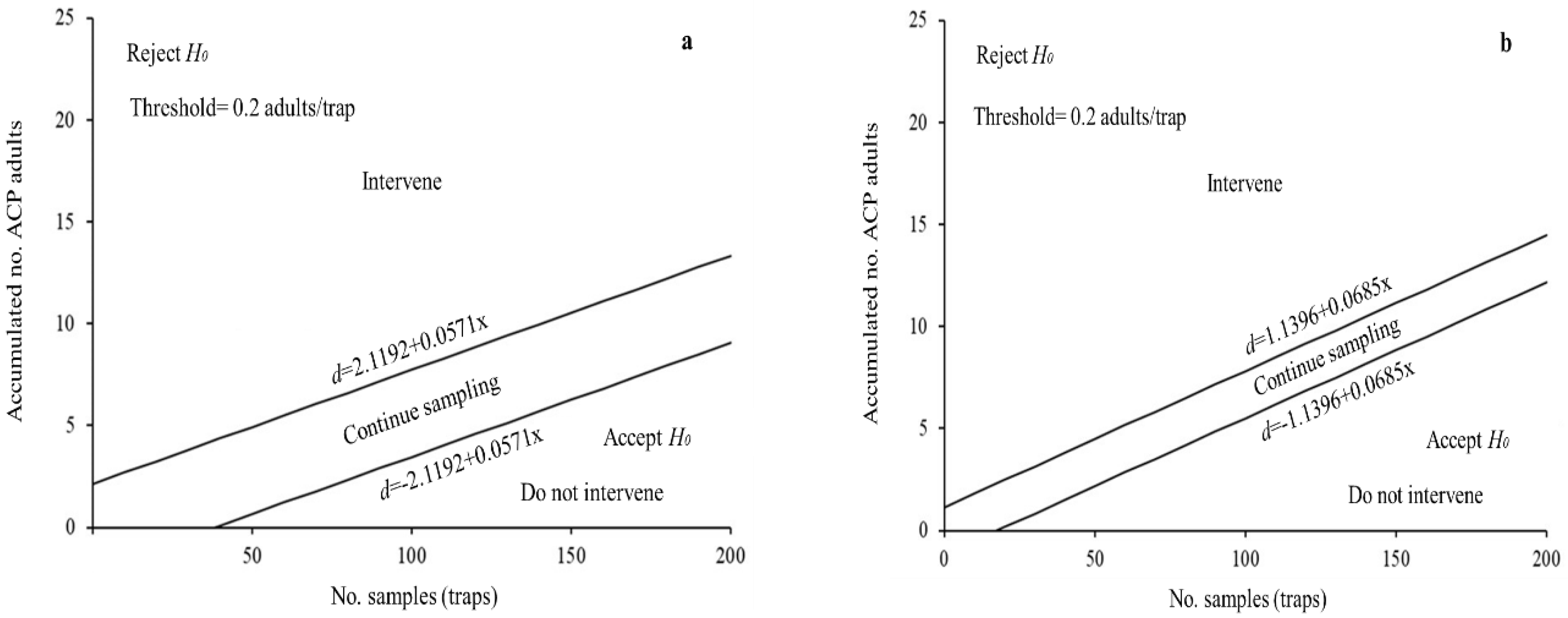
3.4. SPRT Sequential Sampling Plans for D. Citri

With the data analyzed, 18 SPRT sequential sampling plans were obtained for the same number of states out of the total of 24 in the study (Figure 2a,b and

Table 4. Decision stop lines of the SPRT sequential sampling plans for the Asian citrus psyllid for 18 citrus producing states of Mexico, OC, and ASN functions for a threshold = 0.2 adults/trap. α = 0.1, β = 0.1.

State	Stop Lines	MSS	N = 1	OC	ASN
Baja California	d = ±1.3512 + 0.0644x	21	1.4156	0.83	23
Baja California Sur	d = ±1.3796 + 0.0640x	22	1.4436	0.85	24
Chiapas	d = ±1.5435 + 0.0618x	25	1.6053	0.90	28
Hidalgo	d = ±2.1989 + 0.0567x	39	2.2556	0.98	43
Jalisco	d = ±2.3395 + 0.0560x	42	2.3955	0.98	47
Michoacán	d = ±1.1396 + 0.0685x	17	1.2081	0.65	17
Morelos	d = ±1.2401 + 0.0663x	19	1.3064	0.76	20
Nayarit	d = ±2.6591 + 0.0547x	49	2.7138	0.99	54
Nuevo León	d = ±2.3686 + 0.0549x	44	2.4235	0.90	47
Oaxaca	d = ±1.9161 + 0.0584x	33	1.9745	0.96	37
Puebla	d = ±1.3537 + 0.0644x	22	1.4181	0.83	23
Querétaro	d = ±1.4728 + 0.0627x	24	1.5355	0.88	26
Sinaloa	d = ±2.0689 + 0.0574x	37	2.1263	0.97	40
Sonora	d = ±3.3954 + 0.0528x	65	3.4482	1.0	69
Tabasco	d = ±2.1926 + 0.0567x	39	2.2493	0.98	43
Tamaulipas	d = ±3.0703 + 0.0535x	58	3.1238	1.0	62
Veracruz	d = ±2.1192 + 0.0571x	38	2.1763	0.97	42
Zacatecas	d = ±1.4114 + 0.0635x	23	1.4749	0.86	25

MSS = Minimum sample size to determine a density of zero. N = 1: Density to be obtained with the first taken sample to stop sampling and to make a decision to control the vector. OC: Value of the Operational Characteristic at the density of the threshold (0.2 adults/trap). ASN: Average sample number to make a decision at the density of the threshold (0.2 adults/trap). d: estimated ACP density for any given number of samples (traps) (x). x: number of sam-ples (traps).

). The rest were omitted because common k values were not significant or calculable (Table 3). Equations of the stop or decision lines are shown in Figure 2a,b and Table 4. The Ho rejection area is located above the upper line. This rejection area is the point where the decisions to intervene or take action are made if the threshold of 0.2 adults/trap is reached. The acceptance area of Ho is below the lower line. The acceptance area is the point where it is unnecessary to carry out control activities because the estimated density is so low that it will not reach the threshold (Figure 2a,b). Between the two lines is the area of uncertainty. The area of uncertainty indicates that sampling needs to continue until a decision is reached (Figure 2a,b) or the sampling is stopped in accordance with the ASN function, which shows that the number of traps needed to reach a decision with a threshold of 0.2 adults/trap has to be within the range of 17 (Michoacán) to 69 traps (Sonora) (Table 4). According to Oakland [30], when solving the equation for d = 0, we obtain the number of samples needed to determine that the population density is 0. In the case of Michoacán and Veracruz, it is 17 and 38 samples, respectively (Figure 2a,b and Table 4). For the rest of the states, values ranged from 19 to 65 samples (Table 4). The density needed to make a decision from the first sample [30] ranged from 1.2081 (Michoacán) to 3.4482 adults (Sonora) (Table 4). For each of the sampling plans, the Operational Characteristic (OC) and the average number of traps (ASN) were generated for a specified density. Figure 3a,b and Figure 4a,b show such supports for the sampling plans for the 18 determined states. For all of the obtained sequential sampling plans, with the exception of Michoacán and Morelos, the probability to perform a correct intervention with respect to the Operational Characteristic at the threshold considered was >80%. In the states with a high probability value, they are associated with a high number of samples needed in the ASN function to make a decision at the specified threshold (e.g., Nayarit, Tamaulipas, and Sonora) (Table 4, Figure 3a and Figure 4a). The OC curves were steeper in the states with kc values > 0.05 (Figure 3a,b) and a similar response is observed in the ASN curves Figure 4a,b.

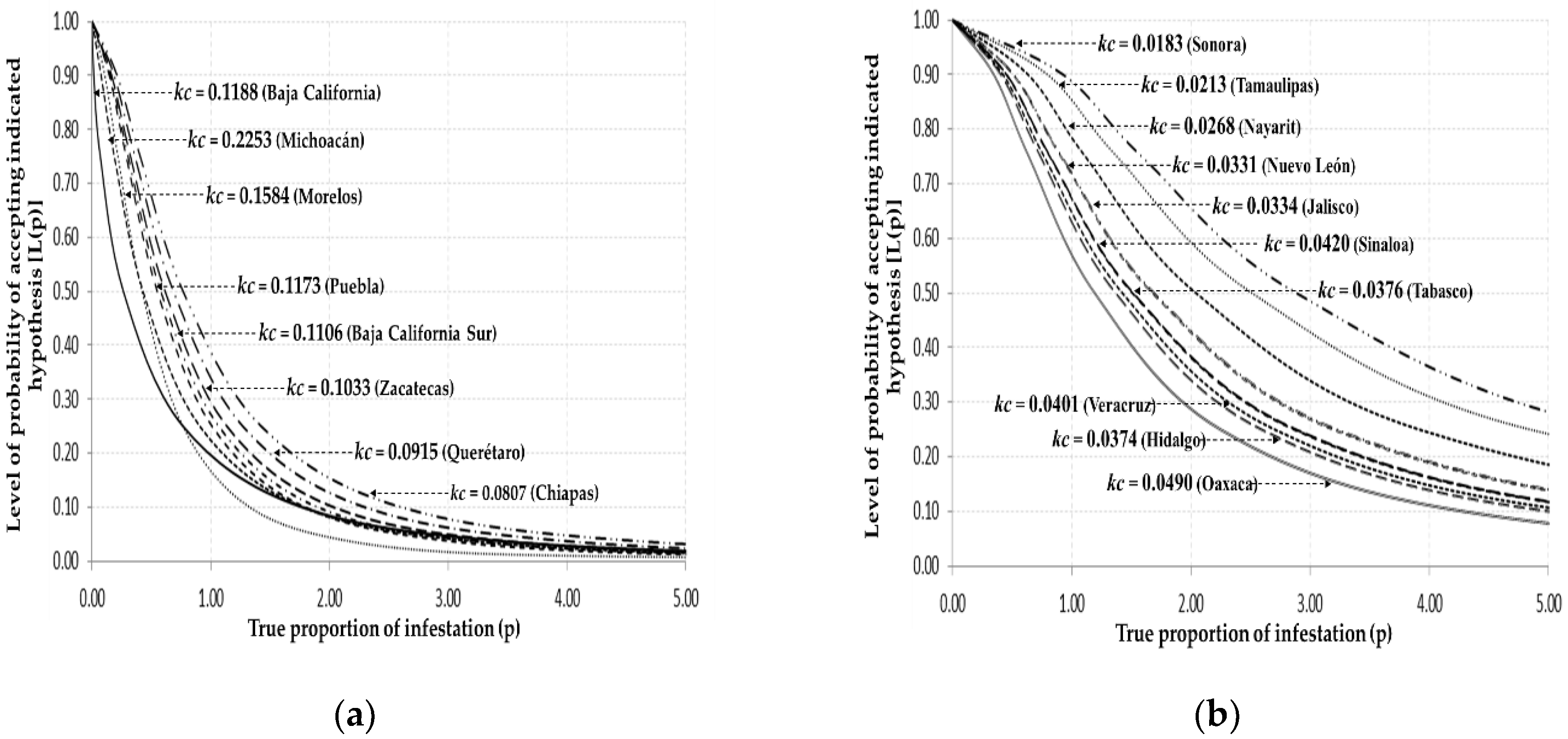
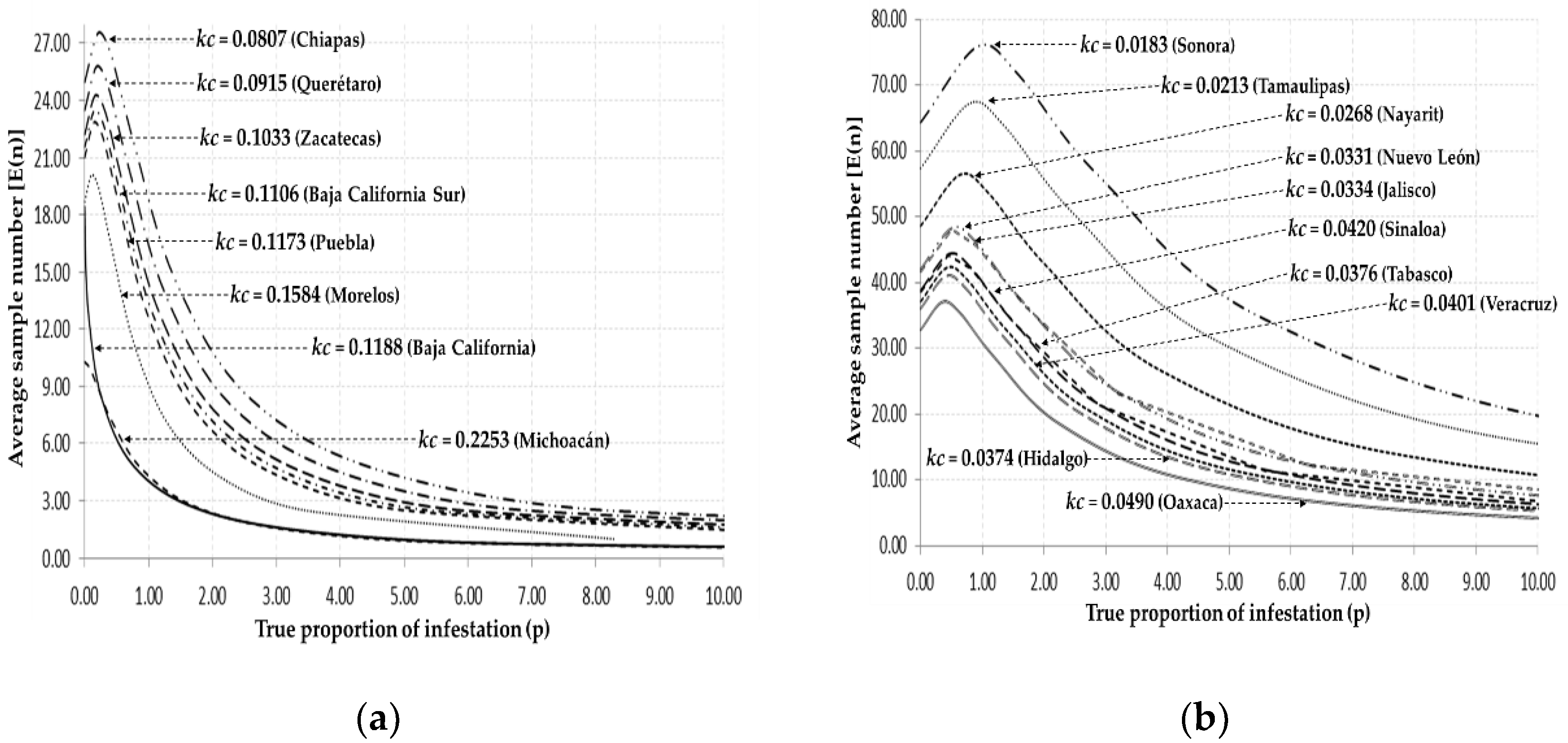
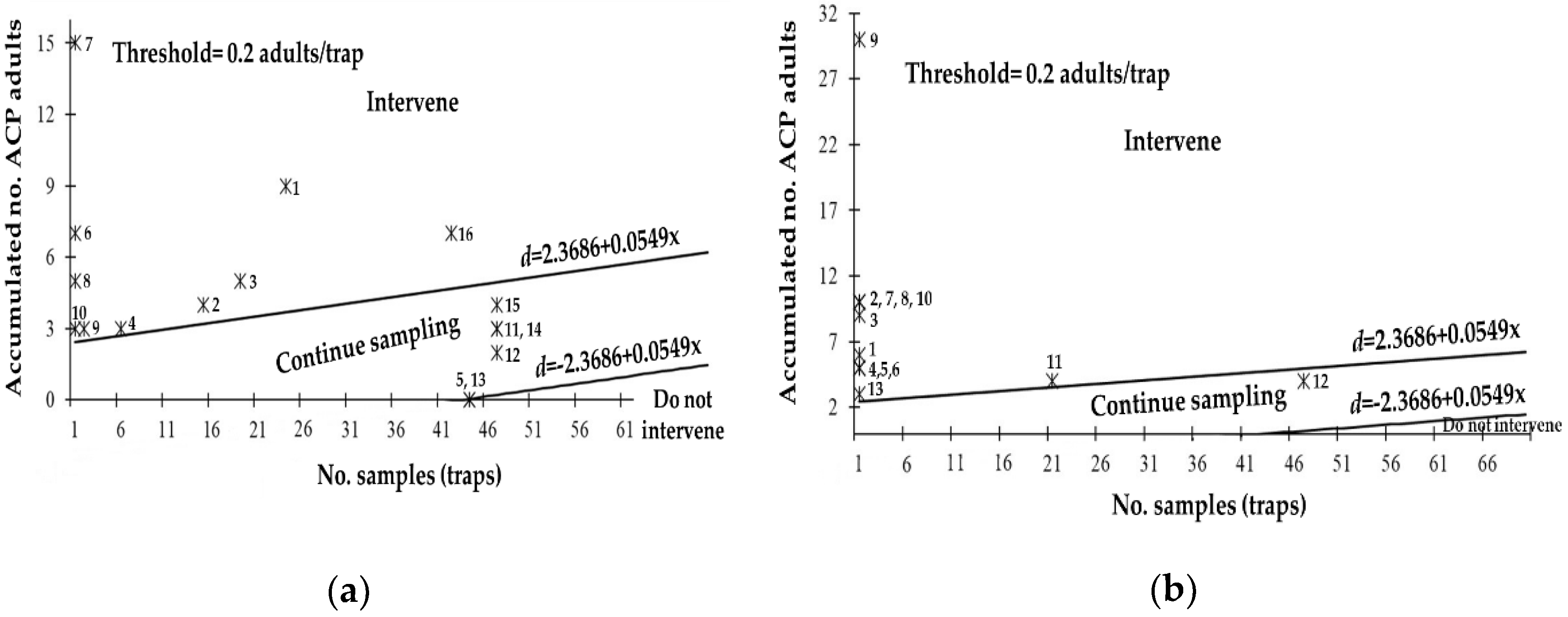
3.5. Field Evaluation of the SPRT Sequential Sampling Plan for D. citri

Field evaluation of the plan was performed at two different sites. In the first citrus grove records covered the period from 17 October 2020 to 15 May 2021. The highest capture of ACP adults in traps ( $\overline{\mathbf{x}}$ = 3.705; SD = 5.471; n = 60) occurred during 11 November 2020 and the lowest ($\overline{\mathbf{x}}$ = 0; n = 60) on 12 December 2020 and 3 April 2021. In total there were 16 sampling dates. Of these, on two dates 44 traps were inspected to confirm zero ACP occurrence (Figure 5a), while on three dates sampling was stopped at 47 counted traps because density of the vector was consistently found in the uncertainty zone (Figure 5a). On four dates, the decision to intervene was reached with the first sample taken because density in the traps was above the threshold of 2.26 ACP adults/trap (Figure 5a). The point of decision making was also reached in five more dates, however, the number of inspected traps ranged 2–42 (Figure 5a). In the second grove, there were only 14 sampling dates with records completed on 3 April 2021. The highest presence of ACP adults in traps ($\overline{\mathbf{x}}$ = 7.117; SD = 5.135; n = 60) occurred during 6 February 2021 and the lowest ($\overline{\mathbf{x}}$ = 0.08; SD = 0.279; n = 60) on 3 April 2021. In 12 out of 14 sampling dates, decision making to intervene was reached with the first inspected trap (Figure 5b). On one date, the decision making point was reached with the tally of 21 traps (Figure 5b). On just one date, the sampling was stopped at 47 inspected traps out of 60 deployed traps because the density of the insects remained in the uncertainty zone (Figure 5b).

4. Discussion

For Mexican citriculture, Taylor’s power law b parameter indicates a highly aggregated distribution for D. citri adults (Table 2). The obtained estimates were significantly >1 (p > 0.001), as was the value found by Monzo et al. [54] whose study used sticky traps in the same manner as our study. Our results were also similar to the indices found by Sétamou et al. [39], with the sampling of shoots in adult orange and grapefruit trees, as well as with the index b = 1.2971 indicated by Tsai et al. [39] that is obtained from the sampling of shoots of Murraya paniculata (L.) Jack. Our values of the parameter b reached a maximum of 3.01 for the case of the Sinaloa state. Although Downing [48] indicates a theoretical range <2, there have been reports in the field indicating a value of b = 3.9 [60]. Taylor et al. [60] indicates that at b > 2, the individuals are more aggregated as the population mean increases. In the case of D. citri, such a response is easily observed in Mexican limes, Citrus aurantifolia (Christm.) Swingle (Michoacán state), where it is common to find high ACP infestations on trees in the orchard and high densities of the insect in the shoots (Table 1). However, the b value obtained in our study differs from the Tsai et al. [39] b value obtained from M. paniculata. As this species is one of the preferred plant hosts of the ACP and regularly shows high densities of the insect [8], the difference is possibly due to the arrangement of the plants in their study, which was conducted over an area of plants (square meter) instead of individual trees. Our data confirm the fit of the mean and variance to Taylor’s power law. Similar results have been found by Rakhshani and Saeedifar [61] for D. citri.

Regarding common k, values obtained in this study were in the range of those reported by Costa et al. [62], who also utilized the Bliss and Owens methodology [51]. However, they differ from the reports by Tsai et al. [38] and Sétamou et al. [39], although, in those studies the calculation of the common k was different. Southwood and Henderson [37] indicate that a general value is around 2, while according to Bliss and Owen [51], kc should be positive and close to zero. In our study the estimates fell into this range. There are studies in which a nominal or arbitrary value of kc is used [63]. In our case, the value was derived from the Bliss and Owen methodology [51] and we validated their different procedures to calculate kc (Table 3). As Nyrop and Binns state [63], the OC and ASN are indicators of the precision of the sampling plans. In our study, there were noteworthy results for both functions in the range of kc > 0.05 (range: 0.0807–0.2253). With high probability for correct intervention at the established threshold and sample size being relatively small, our calculated kc could indicate that there is a good estimate for D. citri in this range. On the other hand, there is also an outstanding response for both functions at the value of kc = 0.049 that was obtained for Oaxaca state (Table 4; Figure 3a,b and Figure 4a,b).

In the obtained values of kc, we noticed a response similar to the one shown by Nyrop and Binns [63], whose results indicated that kc is higher at high densities as well as the existence of a trend in its increase as the population density grows (Table 1, Figure 3a,b and Figure 4a,b). They also specified the changes observed in the form of the OC and ASN functions depending on the value of kc, which were steeper and shifted to the left along the mean density when the value of kc was higher (Figure 3a and Figure 4a) or flatter and shifted to the right when such value was lower (Figure 3b and Figure 4b). In our study, the citrus producing states that showed a high kc value had high probability values for a correct decision for intervention in the OC function, while the number of samples needed to make a decision was relatively low in the range of 8–27. On the contrary, the states with a minimum kc value had higher probability values for a correct decision for intervention in the OC function, while the number of samples needed to make a decision was almost three times as high compared to the high kc value group (Table 4, Figure 3a,b, and Figure 4a,b).

There are implications for studies that determine a single common k value and the possibility of making mistakes [63,64,65]. These are the possible scenarios of error when selecting a common k value for D. citri: (1) in places that select a high kc value where there are no high population densities of the insect, the consequence will be that a reduced number of traps will be inspected and the tally of specimens would probably not be sufficient to reach the threshold. Thus, the decision “do not intervene” will be erroneously made when examining a greater number of traps could yield insect densities that signal intervention and, therefore, making a correct decision. (2) In the opposite situation, under a selection of a lower kc value, making a mistake is remote. As the decision making tool will indicate the need to inspect a high number of traps while the vector population is high, even tallying the insects on a reduced number of traps will result in the threshold being reached and the correct decision to implement control measures against the insect being made. The whole process will be performed without the need to inspect the high number of traps suggested by the ASN function under this assumption. Warren and Chen [64] also mention the importance of considering a possible geographic variation for the same species in the kc value. In our study, there is no response pattern that could support the above. There is variation in the kc value for the same geographical area and the same occurs with limes produced in states in the Pacific coastal region (e.g., Michoacán and Oaxaca) and sweet citrus in the north, south, west, and east of the country (e.g., Sinaloa, Tabasco, Tamaulipas, and Veracruz), but this seems to be more associated with the diversity in the management of the insect and the agroclimatic variations of the location as opposed to a possible genetic trait of the population. In the country, there are three determined haplotypes of D. citri [66] with one widely distributed (Dcit-01), which also occurs indistinctly in the states with variation in the estimated kc values.

For the pattern found in the OC in our study and for the value of the established threshold, it is possible that the established low values of such critical density had determined the indicated results (Figure 4a,b and Table 4); the situation of dealing with a vector of a lethal pathogen in trees obligated to use it. Prager et al. [42], in their study concerning the sampling plan for Bactericera cockerelli-peppers-Ca. Liberibacter solanacearum, a pathosystem similar to that of our study with the difference in the cycle of the plants (annual (pepper) vs. perennial (citrus)) indicated the problems related to the management of a pest that at a minimum density, such as the presence of a single infective insect, would be enough to cause disease in plants, as it is the case in many diseases caused by phytopathogen viruses [3]. For D. citri-citrus-Ca. Liberibacter asiaticus, such threshold is not applicable because studies have shown low transmission associated with a single D. citri adult [11] and even more when nymphal development occurs in healthy plants [9,13,67]. Furthermore, there are diverse natural enemies contributing to the reduction in the vector population [68,69,70,71] that would potentially and naturally assist the prevention of the vector from reaching efficient transmission levels. Hence, it is feasible to consider the use of SPRT sequential plans to support decision making in vector control. However, it is imperative to take into consideration that due to the results obtained in the citrus industry in Brazil, by containing the disease through reducing vector populations among other methods [22] and the contrasting situation of the Florida citrus industry with high rates of infection and relatively abundant presence of the vector [20,72], under the critical densities established in our study, plant infection will probably continue to be obtained with the approach of making decisions with the SPRT sequential sampling plan to intervene against the vector. Nevertheless, what is important for citrus and its growers is to provide tools to reduce this situation and, above all, decrease the economic and environmental costs associated with the frequent application of chemical insecticides to maintain low vector densities. Our results in the field evaluation could provide support for this matter. As noticed in grove 1 (Figure 5a) where, from 16 potential interventions following the generated sequential sampling plan, there were 10 dates that required vector control, while in six it was unnecessary. This represents 37.5% in savings for ACP management. In grove 2 (Figure 5b), there was a different response pattern. Mainly, it was due to a poor selection of insecticides. In consequence, ACP population reduction was not attained and, in most of the sampling dates, the decision making was to intervene. Interestingly, such action was indicated most of the time from a sample size of just one trap (Figure 5b) determined by the high abundance of ACP adults. This represents savings in the sampling effort. This situation would probably be frequent and, under such scenario, the sample size would be equal or lower than the one determined by Tsai et al. [38] and Sétamou et al. [39]. The result would be different when the accumulated density found during the sampling falls into the uncertainty zone where a higher number of samples would be required to reach a decision (Table 4) [27,28,63,73]. A higher number of samples also is required to determine the zero abundance of the vector (Table 4). Nonetheless, under this scenario, to inspect such traps could give more confidence to the grower with respect to the presence of the insect in her/his grove, resulting in a beneficial aspect of the sampling plan.

As stated before, one attribute in sequential sampling is the reduction in the number of samples [27,28,29,30,31,32]. Our sampling plan does not permit this action completely. This is because it is based on the use of a fixed number of sticky traps deployed for vector monitoring [74,75]; however, in addition to taking advantage of this practice, our plan does not require the inspection of the total number of used traps and, in this manner, generates savings in the inspection efforts. Such quantity of traps in the monitoring program could be changed using the ASN function (Figure 3a,b). This could be performed through the selection of the maximum number of samples required to make a decision at the specified threshold (Figure 3a,b and Table 4). Nevertheless, it is possible that the objective of the monitoring could not permit such process because ACP monitoring is focused on detecting the occurrence of the insect in the area [74,75]. Further studies will be needed to define a single sample size useful for both techniques. For the sequential sampling plan for D. citri, there is a major advantage with the use of sticky traps. When the vector population is reduced, the use of these tools for sampling is the only reliable method to determine the occurrence of the insect [54,75]. In this regard, it is also necessary to consider the established threshold, which, although the value is low (0.2 adults/trap), it remains relatively conservative. We selected this value because it would produce a number of interventions that could be accepted by growers. We also tested a more rigorous threshold (0.1 adults/trap) (results not included) for the sequential sampling plan. It generated a wider rejection area (high intervention), the uncertainty zone became narrow (displaced by the rejection area), and the acceptance area (no intervention) was notably reduced and resulted in decision making based on small number of samples, very frequent need for ACP control, and a probable rejection of the plan by most of the growers. Nonetheless, we think that such sequential sampling plan with a threshold of 0.1 adults/trap will be used in the future and even with stricter thresholds (e.g., 0.05, 0.01, or 0.001 adults/trap), which could happen when progress in ACP management results in significant population reduction in the area throughout time. Hence, in our study, the small benefits derived from the use of traps for sampling are surpassed remarkably by the contribution of the sequential sampling plan to decision-making in ACP management. Our main approach is to take advantage of this and promote a science-based strategy against ACP as opposed to a simplistic tactic such as the use of calendar-based insecticide applications.

Adoption of the use of the decision making tools presented herein should yield economic, social, and environmental benefits for users in Mexico and other Central and South American countries where the management of the Asian citrus psyllid is in an incipient stage or in the process of reaching the same level of weekly insecticide sprays carried out in Brazil [22]. It is also feasible for other countries where large new areas are open to citrus production or those at risk of invasion of the vector-pathogen such as the Mediterranean region or in places with orchards already initiated or future plantations with material resistant to or tolerant to huanglongbing. In groves already infected, it should help to reduce reinfection rates by the simple population reduction in the bacteriliferous vector [20] or decrease in the bacterial load in the insect population in the area.

We consider that the development shown here may help to reduce vector populations and reduces the risk of pathogen transmission, while moving towards a rational and integrated management of the insect. This avoids intensive and extensive chemical control of the vector such as the program that exists in Brazil [22]. Furthermore, it would increase the opportunity for biological control [68,69,70,71]. In this manner, the current production systems could move towards the sustainable citrus industry of the future.

References

1. Da Graca, J.V. Citrus greening disease. Annu. Rev. Phytopathol. 1991, 29, 109–136. [Google Scholar] [CrossRef]
2. Da Graca, J.V.; Korsten, L. Citrus Huanglongbing: Review, Present Status and Future Strategies. In Diseases of Fruits and Vegetables, 1st ed.; Naqvi, S.A.M.H., Ed.; Kluwer Academic Publishers: Dordrecht, The Netherlands, 2004; Volume 1, pp. 229–245. [Google Scholar]
3. Gottwald, T.R. Current epidemiological understanding of citrus Huanglongbing. Annu. Rev. Phytopathol. 2010, 48, 119–139. [Google Scholar] [CrossRef] [PubMed] [Green Version]
4. CABI. Invasive Species Compendium. Citrus Huanglongbing (Greening) Disease (Citrus Greening). 2021. Available online: https://www.cabi.org/isc/datasheet/16567 (accessed on 15 March 2021).
5. Bové, J.M. Huanglongbing: A destructive, newly emerging, century-old disease of citrus. J. Plant Pathol. 2006, 88, 7–37. [Google Scholar]
6. National Research Council. Strategic Planning for the Florida Citrus Industry: Addressing Citrus Greening Disease; The National Academies Press: Washington, DC, USA, 2010. [Google Scholar]
7. Santivañez, T.; Vernal, P.; Mora, G.; Díaz, G.; López, J.I. Citrus: Marco Estratégico Para la Gestión Regional del Huanglongbing en América Latina y el Caribe; FAO: Roma, Italia, 2014; 72p, ISBN 978-92-5-107711-5. [Google Scholar]
8. Halbert, S.E.; Manjunath, K.L. Asian Citrus Psyllids (Sternorrhyncha: Psyllidae) and greening disease of citrus: A literature review and assessment of risk in Florida. Fla. Entomol. 2004, 87, 401–402. [Google Scholar] [CrossRef]
9. Ammar, E.-D.; George, J.; Sturgeon, K.; Stelinski, L.L.; Shatters, R.G. Asian citrus psyllid adults inoculate huanglongbing bacterium more efficiently than nymphs when this bacterium is acquired by early instar nymphs. Sci. Rep. 2020, 10, 18244. [Google Scholar] [CrossRef] [PubMed]
10. Inoue, H.; Ohnishi, J.; Ito, T.; Tomimura, K.; Miyata, S.; Iwanami, T.; Ashihara, W. Enhanced proliferation and efficient transmission of Candidatus Liberibacter asiaticus by adult Diaphorina citri after acquisition feeding in the nymphal stage. Ann. Appl. Biol. 2009, 155, 29–36. [Google Scholar] [CrossRef]
11. Pelz-Stelinski, K.S.; Brlansky, R.H.; Ebert, T.A.; Rogers, M.E. Transmission parameters for Candidatus Liberibacter asiaticus by Asian citrus psyllid (Hemiptera: Psyllidae). J. Econ. Entomol. 2010, 103, 1531–1541. [Google Scholar] [CrossRef] [PubMed]
12. George, J.; Ammar, E.-D.; Hall, D.G.; Shatters, R.G., Jr.; Lapointe, S.L. Prolonged phloem ingestion by Diaphorina citri nymphs compared to adults is correlated with increased acquisition of citrus greening pathogen. Sci. Rep. 2018, 8, 1–11. [Google Scholar] [CrossRef] [PubMed]
13. Lee, J.A.; Halbert, S.E.; Dawson, W.O.; Robertson, C.J.; Keesling, J.E.; Singerd, B.H. Asymptomatic spread of huanglongbing and implications for disease control. Proc. Natl. Acad. Sci. USA 2015, 112, 7605–7610. [Google Scholar] [CrossRef] [Green Version]
14. Graham, J.; Gottwald, T.; Setamou, M. Status of Huanglongbing (HLB) outbreaks in Florida, California and Texas. Trop. Plant Pathol. 2020, 45, 265–278. [Google Scholar] [CrossRef]
15. Li, S.; Wu, F.; Duan, Y.; Singerman, A.; Guan, Z. Citrus greening: Management strategies and their economic impact. HortScience 2020, 55, 604–612. [Google Scholar] [CrossRef] [Green Version]
16. Hall, D.G.; Richardson, M.L.; Ammar, E.-D.; Halbert, S.E. Asian citrus psyllid, Diaphorina citri, vector of citrus huanglongbing disease. Entomol. Exp. Appl. 2013, 146, 207–223. [Google Scholar] [CrossRef]
17. Qureshi, J.A.; Kostyk, B.C.; Stansly, P.A. Insecticidal Suppression of Asian Citrus Psyllid Diaphorina citri (Hemiptera: Liviidae) Vector of Huanglongbing Pathogens. PLoS ONE 2014, 9, e112331. [Google Scholar] [CrossRef] [Green Version]
18. Stansly, P.A.; Arevalo, H.A.; Qureshi, J.A.; Jones, M.M.; Hendricks, K.; Roberts, P.D.; Roka, F.M. Vector control and foliar nutrition to maintain economic sustainability of bearing citrus in Florida groves affected by Huanglongbing. Pest Manag. Sci. 2014, 70, 415–426. [Google Scholar] [CrossRef]
19. Boina, D.R.; Bloomquist, J.R. Chemical control of the Asian citrus psyllid and of huanglongbing disease in citrus. Pest Manag. Sci. 2015, 71, 808–823. [Google Scholar] [CrossRef] [PubMed]
20. Singerman, A.; Rogers, M.E. The economic challenges of dealing with citrus greening: The case of Florida. J. Integ. Pest Manag. 2020, 11, 1–7. [Google Scholar] [CrossRef] [Green Version]
21. Yuan, X.; Chen, C.; Bassanezi, R.; Wu, F.; Feng, Z.; Shi, D.; Du, Y.; Zhong, L.; Zhong, B.; Lu, Z.; et al. Region-wide comprehensive implementation of roguing infected trees, tree replacement, and insecticide applications successfully controls citrus HLB. Phytopathology 2020, 23, 1–29. [Google Scholar]
22. Bassanezi, R.B.; Lopes, S.A.; de Miranda, M.P.; Wulff, N.A.; Volpe, H.X.L.; Ayres, A.J. Overview of citrus huanglongbing spread and management strategies in Brazil. Trop. Plant Pathol. 2020, 45, 251–264. [Google Scholar] [CrossRef]
23. Stelinski, L.L. Ecological aspects of the vector-borne bacterial disease, citrus greening (Huanglongbing): Dispersal and host use by Asian citrus psyllid, Diaphorina citri Kuwayama. Insects 2019, 10, 208. [Google Scholar] [CrossRef] [PubMed] [Green Version]
24. Andrade, M.; Li, J.; Wang, N. Candidatus Liberibacter asiaticus: Virulence traits and control strategies. Trop. Plant Pathol. 2020, 45, 285–297. [Google Scholar] [CrossRef]
25. Monzo, C.; Stansly, P.A. Economic injury levels for Asian citrus psyllid control in process oranges from mature trees with high incidence of Huanglongbing. PLoS ONE 2017, 12, e0175333. [Google Scholar] [CrossRef] [PubMed] [Green Version]
26. Wald, A. Sequential Analysis; J. Wiley & Sons: New York, NY, USA, 1947; 212p. [Google Scholar]
27. Onsager, J.A. The rationale of sequential sampling, with emphasis on its use in pest management. United States Department of Agriculture, Economic Research Service. Tech. Bull. 1976, 158539, 1–19. [Google Scholar]
28. Fowler, G.W. Accuracy of sequential sampling plans based on Wald’s sequential probability ratio test. Can. J. For. Res. 1983, 13, 1197–1203. [Google Scholar] [CrossRef]
29. Binns, M.R.; Nyrop, J.P.; van der Werf, W. Sampling and Monitoring in Crop Protection: The Theoretical Basis for Developing Practical Decision Guides, 1st ed.; CABI Publishing: Oxon, UK, 2000; 284p. [Google Scholar]
30. Oakland, G.B. An application of sequential analysis to whitefish sampling. Biometrics 1950, 6, 59–67. [Google Scholar] [CrossRef]
31. Kipchirchir, I. An analysis of sequential sampling strategy in pest control based on negative binomial distribution. ICASTOR J. Math. Sci. 2011, 5, 217–228. [Google Scholar]
32. Pereira, P.S.; Sarmento, R.A.; Galdino, T.V.S.; Lima, C.H.O.; dos Santos, F.A.; Silva, J.; dos Santos, F.R.; Picanço, M.C. Economic injury levels and sequential sampling plans for Frankliniella schultzei in watermelon crops. Pest Manag. Sci. 2016, 73, 1438–1445. [Google Scholar] [CrossRef] [PubMed]
33. Binns, M.R.; Nyrop, J.P. Sampling insect populations for the purpose of IPM decision making. Annu. Rev. Entomol. 1992, 37, 427–453. [Google Scholar] [CrossRef]
34. Flores-Sánchez, J.L.; Mora-Aguilera, G.; Loeza-Kuk, E.; López-Arroyo, J.I.; Gutiérrez-Espinosa, M.A.; Velázquez-Monreal, J.J.; Domínguez-Monge, S.; Bassanezi, R.B.; Acevedo-Sánchez, G.; Robles-García, P. Diffusion model for describing the regional spread Huanglongbing from first-reported outbreaks and basing an area-wide disease management strategy. Plant Dis. 2017, 101, 1119–1127. [Google Scholar] [CrossRef] [PubMed]
35. García-Ávila, C.J.; Trujillo-Arriaga, F.J.; Quezada-Salinas, A.; Ruiz-Galván, I.; Bravo-Pérez, D.; Pineda-Ríos, J.M.; Florencio-Anastasio, J.G.; Robles-García, P.L. Holistic Area-Wide Approach for Successfully Managing Citrus Greening (Huanglongbing) in Mexico. In Area-Wide Integrated Pest Management: Development and Field Application, 1st ed.; Hendrichs, J., Pereira, R., Vreysen, M.J.B., Eds.; CRC Press: Boca Raton, FL, USA, 2021; pp. 33–49. [Google Scholar]
36. Pedigo, L.; Zeiss, M.R. Analyses in insect ecology and management. Bul. Entomol. Res. 1996, 87, 219–220. [Google Scholar]
37. Southwood, T.R.E.; Henderson, A.P. Ecological Methods, 3rd ed.; Blackwell Science Ltd.: Oxford, UK, 2000; 592p. [Google Scholar]
38. Tsai, J.H.; Wang, J.J.; Liu, Y.-H. Sampling of Diaphorina citri (Homoptera: Psyllidae) on orange jessamine in southern Florida. Fl. Entomol. 2000, 83, 446–459. [Google Scholar] [CrossRef]
39. Sétamou, M.; Flores, D.; French, J.V.; Hall, D.G. Dispersion patterns and sampling plans for Diaphorina citri (Hemiptera: Psyllidae) in citrus. J. Econ. Entomol. 2008, 101, 1478–1487. [Google Scholar] [CrossRef] [PubMed]
40. Soemargono, A.; Ibrahim, Y.; Ibrahim, R.; Osman, M.S. Spatial distribution of the Asian citrus psyllid, Diaphorina citri Kuwayama (Homoptera: Psyllidae) on citrus and orange jasmine. J. Biosci. 2008, 19, 9–19. [Google Scholar]
41. Krebs, C.J. Ecological Methodology, 2nd ed.; Addison-Wesley Educational: Menlo Park, CA, USA, 1999; 620p. [Google Scholar]
42. Prager, S.M.; Butler, C.D.; Trumble, J.T. A sequential binomial sampling plan for potato psyllid (Hemiptera: Triozidae) on bell pepper (Capsicum annum). Pest Manag. Sci. 2013, 69, 1131–1135. [Google Scholar] [CrossRef] [PubMed]
43. Taylor, L.R. Aggregation, variance and the mean. Nature 1961, 189, 732. [Google Scholar] [CrossRef]
44. Patil, G.P.; Stiteler, W.M. Concepts of aggregation and their quantification: A critical review with some new results and applications. Res. Popul. Ecol. 1974, 15, 238–254. [Google Scholar] [CrossRef]
45. Banerjee, B. Variance to mean ratio and the spatial distribution of animals. Experientia 1976, 32, 993–994. [Google Scholar] [CrossRef]
46. Taylor, L.R. Assessing and interpreting the spatial distributions of insect populations. Ann. Rev. Entomol. 1984, 29, 321–357. [Google Scholar] [CrossRef]
47. Greig-Smith, P. Quantitative Plant Ecology; Academic Press Inc.: New York, NY, USA, 1957; 198p. [Google Scholar]
48. Downing, J.A. Spatial heterogeneity: Evolved behavior or mathematical artifact? Nature 1986, 323, 255–257. [Google Scholar] [CrossRef]
49. Bliss, C.I.; Fisher, R.A. Fitting the negative binomial distribution to biological data. Biometrics 1953, 9, 176–200. [Google Scholar] [CrossRef]
50. Anscombe, F.J. The statistical analysis of insect counts based on the negative binomial distribution. Biometrics 1949, 5, 165–173. [Google Scholar] [CrossRef]
51. Bliss, C.I.; Owen, A.R.G. Negative binomial distributions with a common k. Biometrika 1958, 45, 37–58. [Google Scholar] [CrossRef]
52. R Core Team. R: A Language and Environment for Statistical Computing; R Foundation for Statistical Computing: Vienna, Austria, 2018. [Google Scholar]
53. Lima, C.H.O.; Sarmento, R.A.; Pereira, P.S.; Galdino, T.V.S.; Santos, F.A.; Silva, J.; Picanço, M.C. Feasible sampling plan for Bemisia tabaci control decision-making in watermelon fields. Pest Manag. Sci. 2017, 73, 2345–2352. [Google Scholar] [CrossRef]
54. Monzo, C.; Arevalo, H.A.; Jones, M.M.; Vanaclocha, P.; Croxton, S.D.; Qureshi, J.A.; Stansly, P.A. Sampling methods for detection and monitoring of the Asian Citrus Psyllid (Hemiptera: Psyllidae). Environ. Entomol. 2015, 44, 780–788. [Google Scholar] [CrossRef] [PubMed]
55. Costa, M.G. Distribuição Espacial e Amostragem Seqüencial de Ninfas e Adultos de Diaphorina Citri Kuwayama (Hemiptera: Psyllidae) na Cultura de Citros. Ph.D. Thesis, Universidade Estadual Paulista, Jaboticabal, São Paulo, Brazil, 2009. [Google Scholar]
56. Hall, H.G.; Hentz, M.G. Sticky trap and stem–tap sampling protocols for the Asian citrus psyllid (Hemiptera: Psyllidae). J. Econ. Entomol. 2010, 103, 541–549. [Google Scholar] [CrossRef]
57. Hall, D.G.; Hentz, M.G.; Ciomperlink, M.A. A comparison of traps and stem tap sampling for monitoring adult Asian citrus psyllid (Hemiptera: Psyllidae) in citrus. Fl. Entomol. 2007, 90, 327–333. [Google Scholar] [CrossRef]
58. Auguie, B.; Antonov, A. gridExtra: Miscellaneous Functions for “Grid” Graphics. 2016. Available online: https://cran.r-project.org/package=gridExtra (accessed on 14 July 2018).
59. Wickham, H. ggplot2: Elegant Graphics for Data Analysis, 1st ed.; Springer: New York, NY, USA, 2009; 213p. [Google Scholar]
60. Taylor, L.R.; Taylor, R.A.J.; Woiwod, I.P.; Perry, J.N. Behavioural dynamycs. Nature 1983, 303, 801–804. [Google Scholar] [CrossRef]
61. Rakhshani, E.; Saeedifar, A. Seasonal fluctuation, spatial distribution and natural enemies of Asian citrus psyllid Diaphorina citri Kuwayama (Hemiptera: Psyllidae) in Iran. Entomol. Sci. 2013, 16, 17–25. [Google Scholar] [CrossRef]
62. Costa, M.G.; Barbosa, J.C.; Yamamoto, P.T.; Leal, R.M. Spatial distribution of Diaphorina citri Kuwayama (Hemiptera: Psyllidae) in citrus orchards. Scientia Agric. 2010, 67, 546–554. [Google Scholar] [CrossRef] [Green Version]
63. Nyrop, J.P.; Binns, M.R. Algorithms for computing operating characteristic and average sample number functions for sequential sampling plans based on binomial count models and revised plans for European red mite (Acari: Tetranychidae) on apple. J. Econ. Entomol. 1992, 85, 1253–1273. [Google Scholar] [CrossRef] [Green Version]
64. Warren, W.G.; Chen, P.W. The impact of misspecification of the negative binomial shape parameter in sequential sampling plans. Biometrics 1986, 47, 419–427. [Google Scholar] [CrossRef]
65. Hubbard, D.J.; Allen, O.B. Robustness of the SPRT for a negative binomial to misspecification of the dispersion parameter. Biometrics 1991, 47, 419–427. [Google Scholar] [CrossRef]
66. Fuentes, A.; Braswell, W.E.; Ruiz-Arce, R.; Racelis, A. Genetic variation and population structure of Diaphoria citri using cytochrome oxidase I sequencing. PLoS ONE 2018, 13, e0198399. [Google Scholar] [CrossRef] [Green Version]
67. Ammar, E.-D.; Ramos, J.E.; Hall, D.G.; Dawson, W.O.; Shatters, R.G., Jr. Acquisition, replication and inoculation of Candidatus Liberibacter asiaticus following various acquisition periods on Huanglongbing-infected citrus by nymphs and adults of the Asian citrus psyllid. PLoS ONE 2016, 11, 1–18. [Google Scholar] [CrossRef] [PubMed]
68. Monzo, C.; Qureshi, J.A.; Stansly, P.A. Insecticide sprays, natural enemy assemblages and predation on Asian citrus psyllid, Diaphorina citri (Hemiptera: Psyllidae). Bull. Entomol. Res. 2014, 104, 576–585. [Google Scholar] [CrossRef] [PubMed] [Green Version]
69. Casique-Valdés, R.; Sánchez-Lara, B.M.; Ek-Maas, J.; Hernández-Guerra, C.; Bidochka, M.; Guízar-Guzmán, L.; López-Arroyo, J.I.; Sánchez-Peña, S.R. Field Trial of Aqueous and Emulsion Preparations of Entomopathogenic Fungi Against the Asian Citrus Psyllid (Hemiptera: Liviidae) in a Lime Orchard in Mexico. J. Entomol. Sci. 2015, 50, 79–87. [Google Scholar] [CrossRef] [Green Version]
70. Cortez-Mondaca, E.; López-Arroyo, J.I.; Rodríguez-Ruíz, L.; Partida-Valenzuela, M.P.; Pérez-Márquez, J. Especies de Chrysopidae asociadas a Diaphorina citri Kuwayama en cítricos y capacidad de depredación en Sinaloa, México. Rev. Mex. Ciencias Agríc. 2016, 7, 363–374. [Google Scholar]
71. Peña-Carrillo, K.; González-Hernández, A.; López-Arroyo, J.I.; Mercado-Hernández, R.; Favela-Lara, S. Mophological and genetic variation in Mexican wild populations of Tamarixia radiata (Hymenoptera: Eulophidae). Fl. Ent. 2015, 98, 1093–1100. [Google Scholar] [CrossRef]
72. Singerman, A.; Burani-Arouca, M. Evolution of Citrus Disease Management Programs and Their Economic Implications: The Case of Florida’s Citrus Industry; Department of Food and Resource Economics, UF/IFAS Extension: Gainesville, FL, USA, 2017; 5p. [Google Scholar]
73. Fowler, G.W.; Lynch, A.M. Sampling plans in insect pest management based on Wald’s sequential probability ratio test. Environ. Entomol. 1987, 16, 345–354. [Google Scholar] [CrossRef]
74. Monzó, C.; Stansly, P.A. Monitoring Asian citrus psyllid populations. Citrus Ind. 2015, 96, 10–12. [Google Scholar]
75. Miranda, M.P.; dos Santos, F.L.; Bassanezi, R.B.; Montesino, L.H.; Barbosa, J.C.; Sétamou, M. Monitoring methods for Diaphorina citri Kuwayama (Hemiptera: Liviidae) on citrus groves with different insecticide application programmes. J. Appl. Ento. 2017, 141, 1–8. [Google Scholar] [CrossRef]
Figure 1. Number and geographic distribution of the yellow sticky traps used in the Mexican trapping system for the monitoring of the Asian citrus psyllid.
Agronomy 11 01434 g001
Figure 2. Decision stop lines of the SPRT sequential sampling plans for the Asian citrus psyllid. Threshold = 0.2 ACP adults/trap. (a) Veracruz state. (b) Michoacán state.
Agronomy 11 01434 g002
Figure 3. Average Sample Number (ASN) function of the SPRT sequential sampling plans for the Asian citrus psyllid for 18 citrus producing states of Mexico. α = 0.1, β = 0.1, and threshold = 0.2 adults/trap. (a). kc ≤ 0.05. (b). kc > 0.05.
Agronomy 11 01434 g003
Figure 4. Operational Characteristic (OC) function for the SPRT sequential sampling plans of the Asian citrus psyllid for 18 citrus producing states of Mexico. α = 0.1, β = 0.1, threshold = 0.2 adults/trap. (a). kc ≤ 0.05. (b). kc > 0.05.
Agronomy 11 01434 g004
Figure 5. Stop lines for decision making in the SPRT sequential sampling for the Asian citrus psyllid in Nuevo León state, Mex. (a) Citrus grove 1. (b) Citrus grove 2. 2020 sampling dates: (1) X-27, (2) X-31; (3) XI-14, (4) XI-28; (5) XII-12, (6) XII-26. 2021 sampling dates: (7) I-9, (8) I-23; (9) II-6, (10) II-20; (11) III-6, (12) III-20; (13) IV-3, (14) IV-17; (15) V-5, (16) V-15. Number in the symbol indicates the sampling date. Symbols represent the number of traps at the accumulated number of ACP adults to reach a decision.
Agronomy 11 01434 g005