Simulation Model for Time to Flowering with Climatic and Genetic Inputs for Wild Chickpea

Abstract

Accurate prediction of flowering time helps breeders to develop new varieties that can achieve maximal efficiency in a changing climate. A methodology was developed for the construction of a simulation model for flowering time in which a function for daily progression of the plant from one to the next phenological phase is obtained in analytic form by stochastic minimization. The resulting model demonstrated high accuracy on the recently assembled data set of wild chickpeas. The inclusion of genotype-by-climatic factors interactions accounted to 77% of accuracy in terms of root mean square error. It was found that the impact of minimal temperature is positively correlated with the longitude at primary collection sites, while the impact of day length is negatively correlated. It was interpreted as adaptation of accessions from highlands to lower temperatures and those from lower elevation river valleys to shorter days. We used bootstrap resampling to construct an ensemble of models, taking into account the influence of genotype-by-climatic factors interactions and applied it to forecast the time to flowering for the years 2021–2099, using generated daily weather in Turkey, and for different climate change scenarios. Although there are common trends in the forecasts, some genotypes and SNP groups have distinct trajectories.

1. Introduction

Chickpea (Cicer arietinum L.), the second most cultivated grain legume crop, is grown in more than 50 countries across the globe from subtropical regions in South Asia, East Africa, and Australia to more pole-ward regions of Australia, and temperate North and South America. It occupies more than 13.5 million ha globally (FAOSTAT) [1,2]. Its cultivation is of particular importance to food security in the developing world where chickpea seeds are a primary source of human dietary protein 1 [3]. Its wild progenitor, Cicer reticulatum, is a quantitative long day (LD) plant that exhibits responsiveness to vernalization [4,5]. Domestication resulted in the widespread adoption, early in the domestic crop’s history, of photoperiod-responsive, vernalization-insensitive genotypes suited to spring cropping, which has left modern cultivated chickpea germplasm with greatly depleted genetic diversity [4,6].

The temperature regime and water availability, day length or competition for resources with other crops in rotation set the time limit for the chickpea to reach its reproductive phase [5,7]. The chickpea is sown in spring in temperate areas, such as the Mediterranean, and North America, and grows while the day length and temperature increases. It is planted after the monsoonal rainy season in subtropical regions, such as Queensland Australia, Central and Southern India and Ethiopia, where the dry season begins with cooler temperatures and shorter days. The reproductive phase of the spring-planted chickpea coincides with the end of the dry season in the southern and central parts of India, and is aligned with the decreasing temperature and shortening day in the more temperate northern parts of this country [8,9]. To achieve a consistent yield, the crop duration must closely match the available growing season [10]. Therefore, chickpea breeding has focused on developing varieties differing in their growth duration to be able to adapt to different latitudes and sowing regimes [4,8,11,12]. Using wild chickpea in introgression crosses can achieve this aim.

Chickpea cultivars and landraces originating from different locations, such as the Mediterranean and northern, central and southern India, were adapted to contrasting phenological regulators and thus are temperature sensitive [8]. This information is invaluable for modeling crop performance. For example, ref. [13,14,15] considered climatic factors, such as expected rainfall, to predict the performance of chickpeas in different geographical locations. In this approach, it was assumed that all genotypes respond to the photoperiod immediately after emergence [16], although this may not be physiologically realistic.

Climate change, resulting from the effects of increased greenhouse gas emissions, has, at present, stronger and stronger effects due to the combined effects of higher temperatures, less available water in regions where it is most needed, and more frequent and intense extreme weather events [17]. Given the importance of global agriculture, as well as opportunities for regions such as Russia (a vast area potentially suited to chickpea production), predicting the effects of global warming on local agricultural practices gains high importance [18]. Over twenty general circulation models (GCMs) have been proposed to predict climate changes. These models converge acceptably at the global scale but their outcomes at the regional scale vary considerably; some models even conflict with each other [19]. Crop models allow for forecasting climate change impacts on crop performance [20,21].

Initiation of flowering was studied at different levels in model plants (Arabidopsis thaliana) [22,23] and crops, such as chickpeas [2]. On a molecular level, several flowering time regulation pathways were identified. Various environmental signals, including the photoperiod and vernalization, and endogenous signals, such as the autonomous and circadian clock, are needed for the plant to start flowering. These signals activate the expression of the floral pathway integrator gene FLOWERING LOCUS T (FT), or five of its homologs identified in the chickpea: FTa1, FTa2, FTa3, FTb, and FTc [2,24]. In this paper, another level is considered, namely, the process-based modeling. Crop models developed earlier for crop legumes, such as SSM [13,16], DSSAT [25,26,27,28,29], APSIM [30] and others [31,32], use differential equations to describe the biophysical and biochemical processes, such as photosynthesis, water uptake, etc. The impact of the genotype, soil, weather and economic factors is also taken into account. The effect of weather conditions on the daily rate of progression to the next phenological phase is quantitatively characterized, using concepts such as the heat unit index (HUI) [32], crop heat units (CHI), hydrothermal degrees (DHD) [33], degree days (DD), or biological days (BD) [15]. Both DD and BD could depend on temperature, water content and photoperiod. DSSAT was used to simulate the growth and yield of soybeans [34] and chickpeas [35] among several other crops [36,37,38,39]. Data from a wide range of growth [13,16] and environmental conditions, including Iran [40] and water deficits in India [14], were successfully modeled using SSM. The utilization of existing models is limited by the need for the considerable manipulations required to adapt the DSSAT model to new environments and cultivars [41,42,43,44,45]. Consequently, the demand for new flexible crop models that can adjust to constantly changing varieties is high.

Genome-wide association studies (GWAS) have provided important tools for understanding the genetics of natural variation and agriculturally important traits. For example, the identification of photoperiodic flowering time genes in sorghum [46]; frost tolerance genes in barley (Hordeum vulgare L.) [47]; leaf architecture [48] and resistance to southern leaf blight genes in maize [49]; and several agricultural traits in rice [50] are some recent examples of GWAS on agriculturally important traits in crops. Genotype-by-environment ($G\times E$) interactions can be investigated, using bioclimatic variables at a site of an accession’s origin as a GWAS phenotype; associations found in these studies indicate climatic adaptation [51]. Typical GWAS designs require the controlled planting of replicated accessions, which can quickly become logistically daunting and expensive across many sites.

Crop models may complement GWAS approaches by accounting for the influence of environmental factors [26]. However, the existing models use some “genetic coefficients” instead of actual genomic data [52] to consider genotype influence. This limits the ability of these models to simulate gene-by-environment interactions and to forecast the phenological characteristics of cultivars across different geographical locations and genotypes [15]. Due to the depleted genetic diversity of cultivated chickpeas, there is a compelling need to re-introduce genetic variation into crop lines, which can be achieved by including wild relatives in breeding programs. Mathematical models and tools that combine genetic and climate data to predict agronomic traits will greatly benefit breeders by simulating the performance of any given well-characterized genotype in any given well-characterized environment [53,54].

Recent crop model comparison under the Agricultural Model Intercomparison and Improvement Project (AgMIP) framework [55,56] revealed that one model is not enough to make forecasts in a changing climate, due to the increasing uncertainties in model predictions with elevated future temperatures [57,58]. Consequently, studies employing ensembles of crop models that give valuable information about model accuracy and uncertainty are needed. Four crop models, as well as their ensemble, were used to simulate an attainable soybean yield in Southern Brazil [31]. Ensemble simulations, such as the mean or median of simulated values, gave better results than any individual model of 27 wheat models tested in four contrasting locations for their accuracy in simulating multiple crop growth and yield variables [58]. To improve the accuracy in the investigation of the elevated ${\mathrm{CO}}_2$ effect on wheat, four models were calibrated to the observed data in [59].

In this work, we applied an approach to model building developed earlier and used to model the flowering time in Vigna radiata [60]. We developed a new dynamical model using the flowering time of two species of wild chickpeas (Cicer reticulatum L. and C. echinospermum) collected at 21 different sites in Turkey and grown in 4 distinct environmental conditions. In contrast to our previous study that used a non-linear regression approach [61], the new dynamical model uses the daily values of climatic factors and GWAS results for genetic information and genotype-by-environment interactions to model a daily progression rate from sowing to flowering. We further used the model to validate the hypothesis of adaptation of genotypes to environmental factors at the geographic origin. Finally, we constructed an ensemble of models using bootstrap resampling, and used it to forecast the time to flowering for the years 2021–2099, using generated daily weather in Turkey. Though chickpea is a promising crop for Russia, forecasting was performed for Ankara, Turkey, in order to use the same sowing days and to be able to compare the results with the measured data.

2. Materials and Methods

2.1. The Overview

Our methodology consists of model construction using cross-validation and testing to select the best model with the lowest validation score; investigation of impacts of different factors to the model using a permutation test; collection of the ensemble of models with probable $G\times E$ interactions using Bootstrap resampling; forecast of time to flowering using generated daily weather for Ankara; and different scenarios (see Figure 1).

These steps are further described below.

2.2. Data Set of Wild Chickpeas

The data set consists of wild chickpea (Cicer reticulatum L. and Cicer echinospermum). Accessions were collected at 21 sites in five regions in Turkey by von Wettberg and co-authors [62] (see a map in Figure S1). The data set spans a large elevational gradient such that C. echinospermum populations generally occur at lower elevations than C. reticulatum, and temperatures are higher and rainfall is lower, on average, in low C. echinospermum sites, compared to higher C. reticulatum sites. The three most easterly and highest elevation C. reticulatum sites are distinguished by having the lowest monthly average temperatures (−4.8 to −2.2 ${}^{\circ }$C versus −2.2 to −0.6 ${}^{\circ }$C) in winter; vegetative phase frost in spring is more frequent in these sites.

These wild accessions were planted in climatically distinct sites in Turkey (Sanliurfa and Ankara, autumn- and spring-sowing) and Australia (Floreat, near Perth, WA and Mt. Barker, in extreme southern WA). As they were grown in contrasting environments, the phenotype data on time to flowering are highly diverse.

To build the simulation model for time to flowering, we used 2174 accessions sown in autumn on 290, 294 or 339 day of year (DOY) in Sanliurfa and Ankara (see Figure 1). The time to flowering for this data set ranges from 117 to 221 day (see Figure 2).

We used 2088 samples from the data set sown in spring as a negative control for model testing. Due to the artificial watering conditions not included in the model, these samples cannot be used for model training, validation or testing. The time to flowering ranges from 64 to 152 days for these samples (see Figure S2) [63].

Here, we used the same six suggestive polymorphic sites associated with flowering time identified earlier [64] in 825 out of 2174 accessions (see Figure 1). These 825 accessions of Cicer reticulatum represent 15 out of 21 collection sites (see Table S1). These SNPs were identified as the best SNPs after running a mixed linear model (MLM) in TASSEL, which associated flowering time (phenotype) with the genotypes, using site/year/season as a factor to account for their effect on phenotype (Table S2). Some alleles are fixed in certain collection sites (Table S3).

These SNPs are already prominently figured in the previous paper, where a full description and rationale are presented [61]. We added them into the analysis here to illustrate the much improved power of the new tests in the context of reanalyzing the same exact phenotypic and genetic data used before. Genes related to flowering time, such as CONSTANS-LIKE 3 gene, FLC-like gene, CONSTANS-LIKE 9 gene, FLC EXPRESSOR gene, PTL-like gene and AGL61 gene are found within 5 mb of these SNPs. To access the genotype–environment interactions, we grouped plants into 18 groups—one for each alternative (ALT) and reference (REF) allele combination (ALT/ALT, REF/ALT and REF/REF)—for each SNP.

The data set of the autumn-sown accessions includes 30 distinct combinations of alleles at 6 positions (Table S2) because not all of the $3^6$ combinatorial combinations are found in the sequenced plants. These combinations are hereinafter referred to as genotypes by the number assigned in the last column of Table S2. The same genotypes may originate from different collection sites, and several genotypes may be found at one site. Genotype #1 corresponds to unsequenced accessions, collected around Siverek village (see a map in Figure S2).

2.3. Climate Data

The data on climatic conditions for each day in the period of field experiments were taken from a publicly available site https://rp5.ru/Weather_in_the_world accessed on 10 September 2019 (the website provides weather forecasts for 172,500 locations as well as observational data reported from weather stations) and NASA [65] (these data were obtained from the NASA Langley Research Center (LaRC) POWER Project funded through the NASA Earth Science/Applied Science Program):

1. 

D is day length.

2. 

$T_n$ is minimal temperature.

3. 

$T_x$ is maximal temperature.

4. 

P is precipitation.

5. 

S is solar radiation.

The measurements for these factors, such as minimal and maximal temperatures (${}^{\circ }$C), are provided for each day as floating point values.

2.4. A Model with Climatic Factors

We model an impact $v(i,t)$ of the weather conditions $X\left(t\right)$ at each day $t,t=0,\dots ,m_i$ on the fitness u of a plant $i,i=0,\dots ,I-1$ to start flowering as the linear combination of N non-linear control functions that depend on climatic factors (1):

$$v(i,t)=\sum _{n=0}^{N-1}{\beta }_n·F_n\left(X\left(t\right)\right)$$

(1)

where ${\beta }_n,n=0,\cdots ,N-1$ are coefficients; $F_n,n=0,\cdots ,N-1$ are non-linear control functions; vector $X\left(t\right)=(D\left(t\right),T_n\left(t\right),T_x\left(t\right),P\left(t\right),S\left(t\right))$ combines climatic factors; and I is the number of plants.

Consequently, the plant’s fitness to start flowering at each day can be written as follows:

$$u(i,t)=u(i,t-1)+H\left(v\right(i,t\left)\right)v(i,t)u(i,0)=0$$

(2)

where $H\left(\right)$ is a Heaviside function. The number of days to flowering $m_i$ predicted by the model is defined by (3):

$$m_i:u(i,m_i)\ge Uu(i,m_i-1)<U$$

(3)

where U is the fitness threshold that the plant needs to reach to be able to flower; $v(i,t)$ depends on the environment at day t; and the interaction of the plant with the environment, $v(i,t)$, can be considered the resource accumulation rate of a plant. Several forms of dependence are proposed in the literature. We propose a more general approach in which this function is determined automatically in analytic form.

2.5. Genotype-to-Climatic Factors Interactions

Formula (1) represents only the influence of climatic factors on the time to flowering. In [52], the framework was developed for combining weather and SNP data. We further enhance the method by introducing non-linearity and automatic function selection. Our genetic information (Table S2) defines groups of samples with allele combinations. We denote K number of SNP and $J=3$ combinations of alternative (ALT) and reference (REF) alleles ALT/ALT, ALT/REF and REF/REF by $C\left(0\right)=AA$, $C\left(1\right)=AR$, and $C\left(2\right)=RR$, respectively. Then, to include the GWAS results into the model, we define $J·K$ groups of plants so that members of the same group have the same combination of alleles in one of the SNP positions (4).

$$\begin{array}{ccc}\hfill \mathrm{SNP}\_\mathrm{k}\_\mathrm{C}{\left(\mathrm{j}\right)}_i& =& \left\{\begin{array}{cc}1\hfill & \mathrm{if}\mathrm{in}\mathrm{plant}i\mathrm{the}\mathrm{combination}\mathrm{for}\mathrm{SNP}k\mathrm{is}j\hfill \\ 0\hfill & \mathrm{otherwise}\hfill \end{array}\right.\hfill \end{array}$$

(4)

A model then takes the following form:

$$\begin{array}{ccc}\hfill v(i,t)& =& \sum _{n=0}^{N-1}\left({\beta }_n+\sum _{k=0}^{K-1}\sum _{j=0}^{J-1}H(|{\beta }_{(3k+j+1)N+n}|\right.\hfill \\ \hfill & -& B_{min}){\beta }_{(3k+j+1)N+n}·\mathrm{SNP}\_\mathrm{k}\_\mathrm{C}{\left(\mathrm{j}\right)}_i)\hfill \\ & ·& F_n\left(X\left(t\right)\right)\hfill \end{array}$$

(5)

where new coefficients ${\beta }_{(3k+j+1)N+n}$ define the effect of genotype-by-climatic factor interaction, and $B_{min}$ is the minimal coefficient value. Thus, the form of the function adapts to the allele combination of a plant by changing the weights of the control functions.

The six polymorphic sites define 18 SNP groups, and thus the number of coefficients for genotype-by-climatic factor interactions equals to 90 for $N=5$ climatic control functions.

2.6. Analytic Form of the Control Function

Several forms of control functions have been proposed in the literature. Here, we propose a more general approach in which the control functions are determined automatically in analytic form, using grammatical evolution (GE) [66,67]. In GE, the analytic function form is built by decoding the sequence called “word” of W integers called codons. Decoding is performed according to simple rules of substitution that establish a correspondence between codons and either an elementary arithmetic operation, ‘+’, ‘−’, ‘*’, ‘/’, or an expression, X, $(X-X^b)$, $1/(X-X^b)$, where X is a name of a climatic factor and $X^b$ is a constant base value of this factor. These constants are specific to factors, so there are $T_x^b$ base maximal and $T_n^b$ minimal temperatures, $P^b$ precipitation, $D^b$ day length and $S^b$ solar radiation.

2.7. Model Adaptation

The vector of model parameters $\theta$ include coefficients ${\beta }_n,n=0,\cdots ,N-1$ and ${\beta }_{(3k+j+1)N+n}$ together with fitness threshold U, the minimal coefficient value $B_{min}$, W GE codons (integer numbers, see Section 2.6) and constants $T_x^b$, $T_n^b$, $P^b$, $D^b$ and $S^b$.

Parameters are inferred automatically by stochastic minimization of the deviation of the model output from data (Formula (6)).

$$\begin{array}{ccc}\hfill Q(\theta )& =& \sum _{i=0}^{I-1}{({\tau }_i-m_i\left(\theta \right))}^2\hfill \\ \hfill & +& \lambda \left\{\sum _{n=0}^{N-1}\left(|{\beta }_n|+\sum _{k=0}^{K-1}\sum _{j=0}^{J-1}\left|{\beta }_{(3k+j+1)N+n}\right|\right)\right\}\hfill \\ & +& \alpha \left\{\sum _{n=0}^{N-1}\left({\beta }_n^2+\sum _{k=0}^{K-1}\sum _{j=0}^{J-1}{\beta }_{(3k+j+1)N+n}^2\right)\right\}\hfill \end{array}$$

(6)

where $\alpha$ and $\lambda$ are regularization parameters, ${\tau }_i$ and $m_i\left(\theta \right)$ are a number of days from planting to flowering measured experimentally and predicted by the model with parameters $\theta$, respectively. Regularization parameters $\alpha$ and $\lambda$ were set to small values (${10}^{-5}$) to limit the effect of penalty in terms in the objective function.

The differential evolution entirely parallel (DEEP) method [68,69] was used in this work. Differential evolution was proposed by Storn and Price in 1995 as a heuristic stochastic optimization method [70]. DEEP was developed by us for application in the field of bioinformatics [68,71]. It includes several recently proposed enhancements [72].

2.8. Model Cross-Validation and Negative Control

The work started by fitting the model (1) to the data set of autumn-sown accessions. To obtain a model with better predictive ability, a 4-fold cross-validation of the model was performed. The whole data set containing 2174 plants was split into training, validation and test sets. To assess the model ability to predict the time to flowering in prospective data sets, we saved 200 randomly selected records as the test set. Then, 3/4 of the remaining records were randomly selected for training and 1/4 for validation. The split was performed 100 times; the model was fitted to the training set and the accuracy of prediction was estimated on a validation set as a root mean error in time to flowering between the predictions and data. Next, the best model with the smallest prediction error was selected and tested on the test set (model M, see Figure 1). The insignificant difference in mean square errors in the time to flowering for the training and validation sets in cross-validation runs and the high-prediction accuracy of flowering time in the test data set ensures that the model was not overfitted and can be generalized to independent prospective data sets.

The set of 2088 spring-sown samples with time to flowering depending on artificial experimental conditions was used for a negative control test, which is considered successfully passed if the model adaptation fails (see Figure 1).

2.9. Estimation of Impacts of Climatic Factors and Genotype Information to the Model

A permutation test was performed to analyze the contribution of climatic factors $T_x$, $T_n$, P, S and D to time to flowering. The essence of the method is to rearrange the data of the factor of interest between dates and record the change in the error. The impact of the climatic factor is then an average error increase over all the permutations. The impacts are then normalized and converted to percentages over all factors (see Figure 1).

To assess the impact of genotype information on flowering time prediction, we fitted a model with $G\times E$ interactions (5) to the same data set, using the same 4-fold cross-validation approach with 100 splits (see Section 2.8). The percentage of increase in the average score for validation runs between models with and without genotype information can be considered the estimate of the impact of the these interactions to the model accuracy. Such an estimate uses information from over 100 runs for both cases, i.e., with and without genotype information, and thus is more reliable than, for example, the estimate using one best model and the test set.

2.10. Model Ensemble with Defined Interactions for Forecasting

In order to make forecasting with our model more reliable, we constructed an ensemble of models with a fixed analytic form of control functions obtained in cross-validation runs for model (1) (see Section 2.8). To be able to statistically analyze the estimates of the influence of genotype-by-environment interactions to time to flowering and calculate the confidence intervals, the coefficients ${\beta }_{n:n\ge N}$ were estimated using the Bootstrap resampling method [73]. In brief, model adaptations were performed using data sets resampled from the original one with repetitions, i.e., some samples may have been omitted while others were duplicated. We applied a Mann–Witney–Wilcoxon criterion to the resulting samples of each parameter ${\beta }_{n:n\ge N}$ to find coefficients that were significantly non-zero.

The following heuristic procedure was applied to construct the ensemble of models for forecasting. The resulting empirical distributions for each parameter ${\beta }_{n:n\ge N}$ are represented as histograms, and the most probable parameters belong to the highest bins of the histogram. Consequently, the models with the majority of parameters with this property are considered the best models and selected into the ensemble. We required that more than 97.5% of coefficients ${\beta }_{n:n\ge N}$ belonged to the highest bins in the histogram.

2.11. Synthetic Weather Generation and Time to Flowering Forecast

The daily weather forecasts for Ankara, Turkey, were produced, using the weather generator program MarkSim, covering the period between 2021 and 2099 years. To achieve better results, 30 replications were recorded. MarkSim was designed to simulate weather from known sources of monthly climate data [74,75,76,77]. MarkSim implements several global models and takes into account the socio-economic development scenarios described by the four representative carbon dioxide concentration profiles (RCPs) adopted by the Intergovernmental Panel on Climate Change (IPCC) in the fifth assessment report (AR5) in 2014. The profiles correspond to a wide range of possible changes in future anthropogenic emissions of greenhouse gases and are called rcp26, rcp45, rcp60 and rcp85 in accordance with the possible violation values for radiation earth balance in 2100 with respect to the preindustrial epoch (+2.6, +4.5, +6.0 and +8.5 W/m${}^2$, respectively) [78].

The safest socio-economic scenario for global climate change due to the proposed nature preservation actions is called rcp26. rcp85 is the most dangerous scenario, while rcp45 and rcp60 lay in between these extremes. Following [79], we used GFDL-ESM2M [80] and HadGEM2-ES [81] models to forecast the climate in Ankara, Turkey. HadGEM2 is a comprehensive model of the Earth system developed by the Hadley Center, U.K. The standard atmospheric component has 38 levels extending to a height of 40 km. The horizontal resolution is 1.25${}^{\circ }$ latitude and 1.875${}^{\circ }$ longitude (≈112.5 km) (MetOffice). GFDL-ESM2M is a comprehensive model of the Earth system developed by the Laboratory Geophysical Hydrodynamics (GFDL) of the National Oceanic and atmospheric research (NOAA). This is one of the preferred models in the Coupled Model Intercomparison Project 5 (CMIP5). This version has a resolution of 2.5${}^{\circ }$ longitude, 2${}^{\circ }$ latitude (≈220 km) horizontally and 24 levels vertically.

3. Results

3.1. A Model with Climatic Factors

The model cross-validation and testing were performed to select the best and most reliable model (see Figure 1). The data set was split into training, validation and test sets. The number of samples was 1482, 492 and 200, respectively. Optimization was performed with the training set, and then the model with a lowest score equal to the sum of squared differences between the model solution and data in terms of the number of days from sowing to flowering (18,580.0) for the validation set was selected and run on a test set. The histograms for the training and validation sets are presented in Figure 3.

To verify the validity of the constructed model, we compared the mean values of the root mean scores with a Mann–Whitney–Wilcoxon criterion. The difference between the training and validation scores, 30.7 and 36.6, respectively, was not statistically significant (p = 0.14 $>0.01$).

The best model (7) was selected with parameters ${\theta }_1^{*}$.

$$\begin{array}{ccc}\hfill v(i,t)& =& 4.92·F_0+7.88·F_1+2.59·F_2+1.13·F_3+9.35·F_4\hfill \\ \hfill F_0& =& \frac{T_n}{S}\hfill \\ \hfill F_1& =& T_n-13.5616\hfill \\ \hfill F_2& =& D-7.2458\hfill \\ \hfill F_3& =& \frac{T_n}{D·(T_x-19.6387)}\hfill \\ \hfill F_4& =& \frac{1}{T_n-13.5616}\hfill \end{array}$$

(7)

where $F_n$ are climatic control functions.

$F_0$ shows that the resource accumulation rate increases with positive minimal temperature, but with growing solar radiation, the weight of this term decreases. Linear terms $F_1$ and $F_2$ indicate that increasing minimal temperature by one degree above ≈13.6 ${}^{\circ }$C or day length values by one hour above ≈7 h lead to the increase in the resource accumulation rate by the values of ≈8 or ≈3, respectively. Functions $F_3$ and $F_4$ correct the resource accumulation rate at high temperatures, i.e., slow down the rate increase in this case.

The best model with optimized parameters accurately describes the training and validation data (see Figure 4); the Pearson correlation coefficient is ≈0.98 in both cases.

The model solutions for the validation and test sets closely coincide with the experimental data in terms of the mean, median, maximal and minimal difference in the number of days to flowering (see

Table 1. Error estimates for validation and test. Mean, median, maximal and minimal difference in the number of days to flowering between the model solution and data.

Error Type	Validation (Days)	Test (Days)
Mean	5.0	6.085
Median	4.0	5.0
Maximal	24.0	19.0
Minimal	0.0	0.0
Number of samples	492	200

).

For a negative control test for the model, we used a set of 2088 samples sown in spring (see Figure 1). The time to flowering of these samples cannot be described by the model due to the artificial experimental conditions (i.e., water addition). We performed the same model adaptations and did not find any acceptable parameter combinations. The numerical limit for time to flowering of 152 days is predicted for most samples (see Figure 5).

3.2. Impacts of Different Factors to the Model

To assess the impacts of climatic factors to the model, we performed a permutation test with 100 permutations (see Figure 1). The minimal temperature $T_n$ has a maximal impact on the model—over $85\%$—and the day length impact is $14.4\%$. The impacts of maximal temperature, solar radiation and precipitation are almost negligible—0.02%, 0.08% and 0%, respectively (see Figure 6).

To assess the impact of genotype information, a model with $G\times E$ interactions (5) was built using the same methodology with 4-fold cross-validation and 100 splits (see Figure 1). The root mean sum of squared differences between the model solution and the data in terms of the number of days from sowing to flowering was used as the score (see Figure 7).

The impact of genotype information on model accuracy was estimated as the difference in means between the root mean scores for the validation set for the model (7) (that equals 36.6) and the model with the genotype information (8.6). The decrease in the root mean score for adding the genotype information equals to 28 or 77% of the value for model (7).

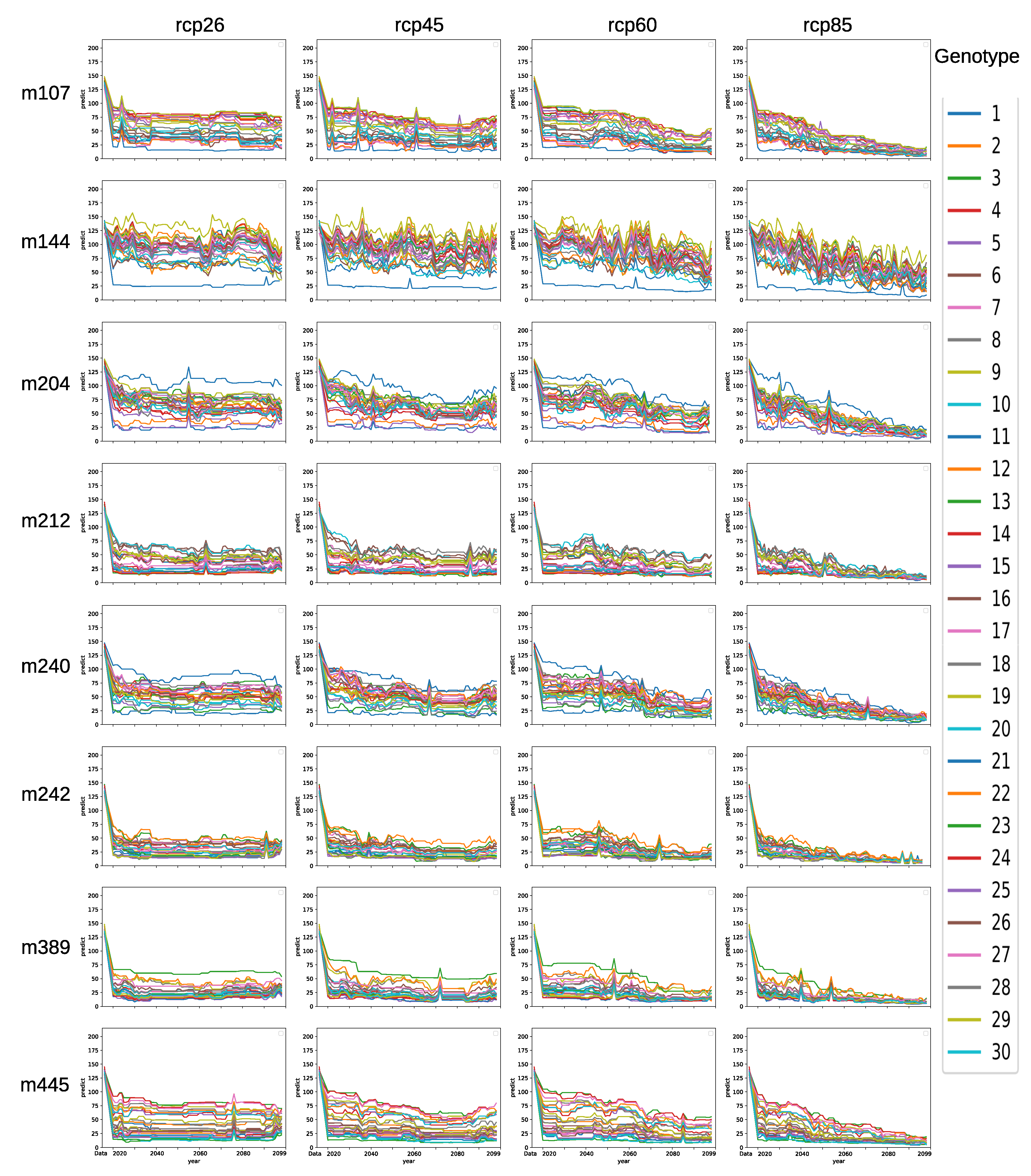
3.3. Comparison of Genotypes

We used the results of the permutation test and applied a Mann–Whitney–Wilcoxon criterion to compare the impacts of climatic factors for all pairs of genotypes (see Table S5). The effect of maximal temperature $T_x$ is the same for all pairs, while the effect of minimal temperature $T_n$ is different for all pairs, except #20–#21 (originated from Egill and Kalkan, respectively), #9–#27 (originated from Barisptepe and Sarikaya, respectively) and #18–#29 (originated from Egill and Besevler, respectively).

The impact of climatic factors varies for accessions from different collection sites (see Section 2.2 and Table S4). The impact of minimal temperature is positively correlated with the longitude at primary collection sites with Pearson’s $r=0.71$ ($p=0.002<0.05$) and Spearman’s $\rho =0.80$ ($p=0.0005<0.05$), while the impact of day length is negatively correlated with longitude with Pearson’s $r=-0.71$ ($p=0.003<0.05$) and Spearman’s $\rho =0.80$ ($p=0.0005<0.05$). The impacts of minimal temperature and day length are correlated in the same way with elevation but with lower significance, $p<0.1$ (see

Table 2. Correlations (Pearson’s r and Spearman’s $\rho$) of impacts of maximal and minimal temperature—$T_x$ and $T_n$, solar radiation S, day length D, with geographical characteristics of collection sites.

	${\mathit{T}}_{\mathit{x}}$	${\mathit{T}}_{\mathit{n}}$	S	D
Longitude	$r=-0.47$ ($p=0.08>0.05$) $\rho =-0.14$ ($p=0.62>0.05$)	$r=0.71$ ($p=0.002<0.05$) $\rho =0.80$ ($p=0.0005<0.05$)	$r=0.03$ ($p=0.92>0.05$) $\rho =0.26$ ($p=0.35>0.05$)	$r=-0.71$ ($p=0.003<0.05$) $\rho =0.80$ ($p=0.0005<0.05$)
Latitude	$r=0.34$ ($p=0.22>0.05$) $\rho =-0.05$ ($p=0.87>0.05$)	$r=-0.37$ ($p=0.17>0.05$) $\rho =-0.70$ ($p=0.005<0.05$)	$r=0.13$ ($p=0.64>0.05$) $\rho =-0.39$ ($p=0.15>0.05$)	$r=0.37$ ($p=0.17>0.05$) $\rho =0.70$ ($p=0.005<0.05$)
Elevation	$r=-0.05$ ($p=0.87>0.05$) $\rho =-0.22$ ($p=0.44>0.05$)	$r=0.45$ ($p=0.09>0.05$) $\rho =0.48$ ($p=0.07>0.05$)	$r=0.03$ ($p=0.91>0.05$) $\rho =-0.16$ ($p=0.53>0.05$)	$r=-0.45$ ($p=0.09>0.05$) $\rho =-0.48$ ($p=0.07>0.05$)

). Note that elevation is correlated with longitude with $r=0.66$ ($p=0.007<0.05$) and $\rho =0.70$ ($p=0.004<0.05$).

According to the description of site environments (see Section 2.2 and [62]) the climate is cooler at higher elevations and the day length is limited in valleys surrounded by mountains. Thus, our results can indicate that accessions from highlands are adapted to lower temperatures, while those that are originated in valleys are used to shorter days.

Day length has a significant Spearman’s correlation ($\rho =0.70$, $p=0.005<0.05$) and insignificant Perason’s correlation ($r=0.37$, $p=0.17>0.05$) with latitude. While the difference in latitude between collection sites is relatively low, this can indicate the photoperiod sensitivity of the wild accessions.

The impact of minimal temperature has a significant Spearman’s correlation with latitude and weakly significant correlation coefficients with elevation, while correlations between other pairs of climatic factor impacts and geographical characteristics are statistically insignificant (see Table 2).

For genotypes #27, #17, #10, #9 and #4 (originated from Baristepe, Cudi and Sarikaya) the impact of minimal temperature $T_n$ is over 90%. In contrast, for genotypes #29 and #30 (originated from Besevler, Sarikaya and Kalkan) the effect of $T_n$ is significantly smaller and equals to approximately 70%. The impact of day length D for these two genotypes is about 30%, while all other genotypes have D impact less than 25% (see Table S7).

The comparison of genotypes by reached fitness u (2) is done with a bootstrap approach. We applied a Mann–Whitney–Wilcoxon test to find pairs with statistically significant differences in u. Genotypes #29 and #30 (originated from Besevler, Sarikaya and Kalkan) again differ from all other ones (see Figure 8).

Such diversity in response to environmental factors can be beneficial for breeding programs that can include wild relatives of cultivated chickpea.

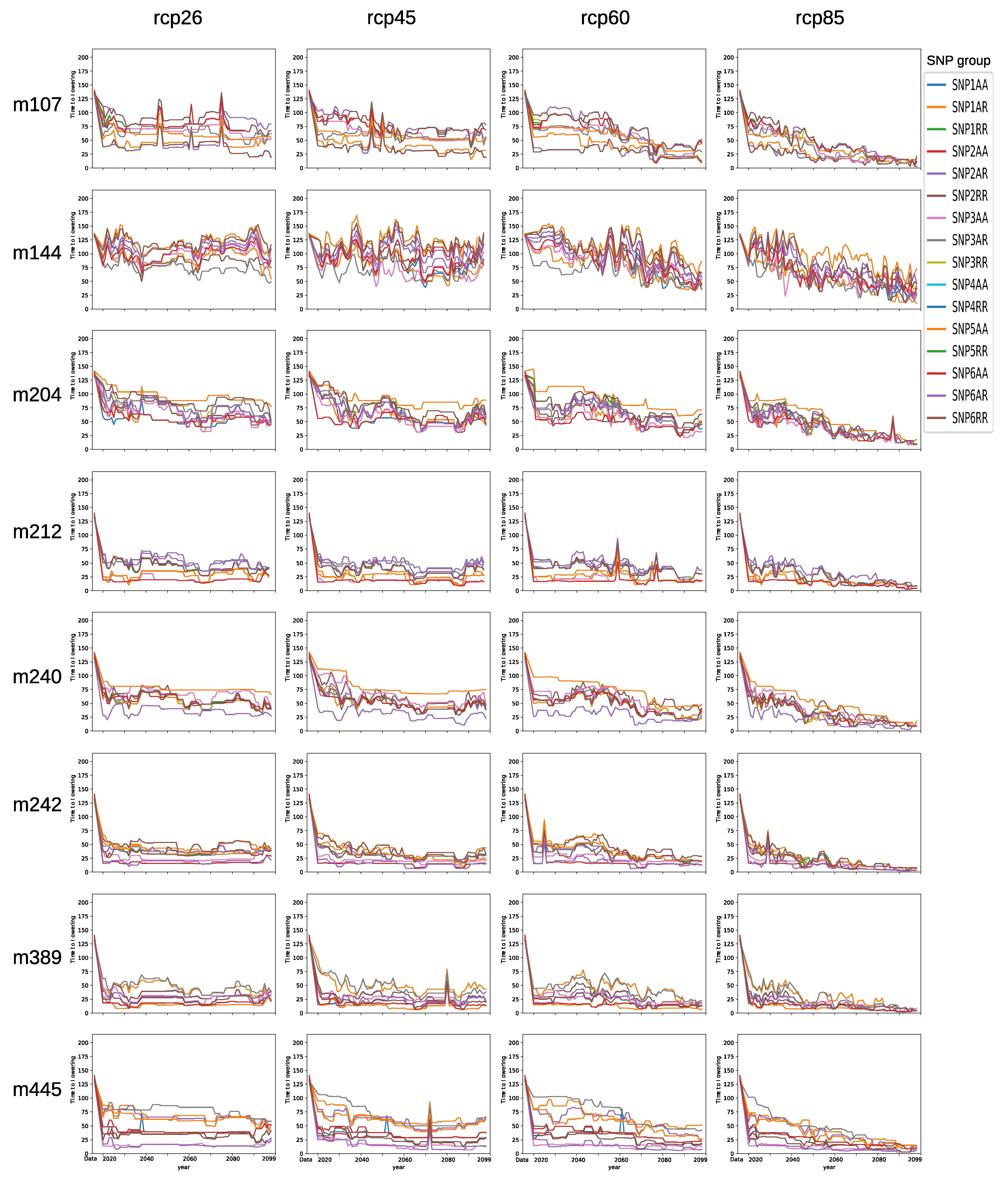
3.4. Comparison of SNP Groups

We used the results of the permutation test and applied a Mann–Witney–Wilcoxon criterion to compare the impacts of climatic factors for different SNP groups (see Table S6). The mean impacts of climatic factors for different SNP groups are approximately the same.

The results of the permutation test showed that the difference in impact to flowering time of minimal temperature $T_n$, solar radiation S and day length D between all pairs of alleles in all SNP groups is statistically significant according to Mann-Whitney-Wilcoxon criterion. In contrast, the difference in impact to the flowering time of maximal temperature $T_x$ is insignificant between all pairs of alleles in all SNP groups.

We used the results of bootstrap test to compare pairs of SNP groups by reached fitness u (2) with a Mann–Whitney–Wilcoxon criterion. A statistically significant difference is found between SNP2AA and SNP2RR (p = 0.000585 $<0.05$), SNP2AR and SNP2RR (p = 0.015765 $<0.05$), SNP3AA and SNP3RR (p = 0.017337 $<0.05$) (see

Table 3. p-Values for comparison of SNP groups by reached fitness u (2) with Mann–Whitney–Wilcoxon test.

SNP1AA vs. SNP1AR	0.193
SNP1AA vs. SNP1RR	0.387
SNP1AR vs. SNP1RR	0.118
SNP2AA vs. SNP2AR	0.448
SNP2AA vs. SNP2RR	0.001
SNP2AR vs. SNP2RR	0.016
SNP3AA vs. SNP3AR	0.363
SNP3AA vs. SNP3RR	0.017
SNP3AR vs. SNP3RR	0.058
SNP4AA vs. SNP4RR	0.096
SNP5AA vs. SNP5RR	0.115
SNP6AA vs. SNP6AR	0.292
SNP6AA vs. SNP6RR	0.351
SNP6AR vs. SNP6RR	0.359

).

3.5. Model Ensemble with Genotype-to-Climatic Factors Interactions

The difference in mean values of the root mean scores between training (7.7 days) and validation sets (8.6 days) (see Figure 7) for the model with the genotype information (see Section 2.5, Formula (5)) was statistically significant according to a Mann–Whitney–Wilcoxon criterion at the level of 5% (p = 0.03) and insignificant at the level of 1%. Thus, the constructed model is weakly validated. This can be explained by the fact that the number of samples with and without genotype in the training and validation sets are not balanced.

In order to construct a reliable model, we applied a bootstrap approach and performed B = 500 model adaptations using data sets resampled from the original one with repetitions (see Figure 1). The analytic form of the climatic control functions was taken to be the same as that found in the model (7) and fixed. We constructed histograms that represent empirical distributions for coefficients ${\beta }_{n:n\ge N}$ for genotype-to-climatic factors interactions.

It was found that 75 out of 90 coefficients are significantly non-zero, according to a Mann–Whitney–Wilcoxon criterion (see Table S7). Interactions of all SNPs with control functions, and, consequently, with minimal day temperature, day length and solar radiation, influence the time to flowering in our model because for any SNP, there are allele combinations for which the coefficients of at least some control functions are statistically and significantly non-zero.

The empirical coefficient ${\beta }_{n:n\ge N}$ distributions are bimodal, as the majority of the values fall into bins adjacent to the boundaries, i.e., $(-10.0;-7.5)$ and $(7.5;10.0)$ (see Figure S3).

Following the heuristic procedure described in Section 2.10, we calculated for each model the number of coefficients ${\beta }_{n:n\ge N}$ in the highest bins and constructed the histogram (see Figure 9) that represented the empirical distribution of the number of such coefficients with mean and standard deviations equal to 55.81 and 4.83, respectively.

In order to select the models containing more than 97.5% of the coefficients from the highest bins, we calculated the threshold value $B=55.81+1.96\times 4.83=65.28$ using the mean, standard deviation of the empirical distribution and the z score 1.96 for the 97.5 percentile.

We selected 8 models with a number of coefficients ${\beta }_{n:n\ge N}$ in the highest bins greater than threshold value B (see Table S8). The ensemble models are of high accuracy (see

Table 4. Error estimates for ensemble models. SSD means sum of squared differences between model solution and data; MEAN and MED represent mean and median deviation of model solution from experimental data in days.

Model Name	SSD	MEAN	MED
m107	117,260.0	5.79	5.0
m144	134,074.0	5.93	5.0
m204	105,133.0	5.26	4.0
m212	106,429.0	5.29	4.0
m240	106,119.0	5.29	4.0
m242	106,228.0	5.29	4.0
m389	119,893.0	5.59	4.0
m445	120,305.0	5.87	5.0

), i.e., the mean deviation of the model solution from the experimental data is less than 6 days.

3.6. Forecasting

To achieve more reliable results, we generated 30 replications of weather forecasts for Ankara for each year from 2021 to 2099, using the MarkSim weather generator for representative carbon dioxide concentration profiles rcp26, rcp45, rcp60 and rcp85 described in Section 2.11 (120 weather forecasts in total). Between 2021 and 2099, an increase in maximum temperature is expected for rcp26 by 0.7 degrees, for rcp45 by 1.5, rcp60 2.5, and rcp85 5.0. Minimum temperature will increase for rcp2.6 by 0.5 degrees, rcp45 by 1.0, rcp60 by 1.5, and rcp85 by 2.5.

Generated weather forecasts were used to predict time to flowering for 30 genotypes and 16 SNP groups, using the ensemble of models for sowing dates DOY 339 and DOY 294 (see Figure 10, Figure 11, Figure 12 and Figure 13, respectively).

For sowing date DOY 339, the time to flowering decreases in the majority of cases, though in some models it can vary (see Figure 10). For all genotypes and for all models, except m144, the time to flowering has the same behavior. Its value for the first year of forecast (2021) is different for each genotype but for all of them it is less than the experimental value measured for the data set. The time to flowering stays approximately at the same level until the last year of forecast (2099) for rcp26. For rcp45, it continues to decrease until 2060–2070 and then stays approximately at the same level or even increases, for example, for model m107 and genotype #1 (unsequenced accessions) and for model m389 and genotypes #22, #9 (originated from Baristepe and Savur); these examples are marked with an asterisk (‘*’) in Figure 10 (see Section 2.2 and Table S2 for genotype numbers). For rcp60 and rcp85, the time to flowering decreases almost monotonically.

The behavior of the genotypes in model m144 differs from that scenario. Genotypes #8, #21, #26 (originated from Baristepe, Kalkan and Sarikaya) and #1 (unsequenced accessions) have a significant drop in the time to flowering between the value measured in the experiment and the year 2021 forecast (this example is marked with two asterisks (‘**’) in Figure 10). The forecasts for later years for Genotypes #8, #21, #1 (originated from Baristepe and Kalkan) are either constant or continue to decrease, while the forecast for Genotype #26 (originated from Sarikaya) increases. The forecasts for time to flowering for other genotypes fluctuate around the value found in the data set for rcp26 and rcp45, and have a trend to decrease for rcp60 and a more significant trend to decrease for rcp85.

For sowing date DOY 339, the trajectories for the time to flowering forecast for different SNP groups show different behaviors (see Figure 11). For models m107, m144, m204 and all RCPs, the trajectories cluster closely together. For models m240 (SNP2AA), m242 (SNP1AA, SNP6AR, SNP3AA), m389 (SNP1RR, SNP2RR, SNP6RR), and m445 (SNP4AA, SNP5AA), one, two or three trajectories do not belong to the main cluster but have a greater drop in the time to flowering between the observed value in the data and year 2021 forecast; they stay separated from other trajectories at the lower level until 2099. Thus, modeling predicts that these SNP groups are the most sensitive to the climate change.

For sowing date DOY 294 for rcp26 for all models except m144 time to flowering drops significantly between an observed value in the data set and year 2021 forecast and later stays approximately at the same levels for all genotypes (see Figure 12 and Figure 13). For rcp45, rcp60 and rcp85 and all models except m144 time to flowering for all genotypes drops significantly between an observed value in the dataset and year 2021 forecast and continues to decrease later for genotypes with relatively bigger forecasted value at 2021 so that for rcp60 and rcp85 all trajectories converge almost in one point at 2099.

4. Discussion

The lifecycle of the chickpea and its phenology is strongly predicted by its geographic origin and local environmental factors as demonstrated for domestic chickpea cultivars and landraces originating from the Mediterranean and southern India [8]. Here, we validate the hypothesis that adaptation to environments at sampling sites is blueprinted in genomes by dynamically modeling the genotype responses to changing climate conditions. Usually, a limited number of genetic coefficients are included in dynamical crop models, such as DSSAT or SSM [52]. We implemented a solution in which the analytic form of the impact of climatic factors and their interactions with genotype to the fitness of a plant to flower is automatically inferred by a stochastic optimization technique. We performed model parameterization on a wild chickpea data set collected at 21 different locations in Turkey [62] grown in two contrasting environments. GWAS analysis of the data identified six polymorphic sites responsible for the flowering time variation, independent of the environmental conditions [64].

The constructed model (7) is similar to that developed in [16] due to the absence of dependency on precipitation in the sowing–flowering period and the possibility to estimate resource accumulation. The model [16] has a linear function for the sowing-emergence interval and is multiplicative—for emergence-flowering. The model (7) is a combination of two types of functions, as only the data on flowering were available. The advantages of our model are the automatically constructed analytic form and the presence of genotype-to-climatic factors interactions.

The absence of dependency on precipitation can be considered a limitation of the constructed model, as watering is important for plant growth [5,7,82]. This can be due to the properties of the available data that include only one phenotype—the time to flowering, measured at two locations. Additional data, such as time to emergence, may improve this situation.

In comparison to regression models developed earlier [61], formula (7) is simpler and thus more interpretative. That is because the daily values of the climatic factors are used as the model input instead of summaries over different periods, which are not always well defined.

The estimated impact of genotype-by-environment interactions on model accuracy amounts to 77%, which is more than four times greater in comparison to [61] (17.2%). This can be due to the model adaptation to a more consistent data set.

Though the amount of accumulated data is constantly growing, the understanding of the role of temperature and day length in adaptation to different habitat types is still incomplete [83]. Our model predicts the diversity in response to climatic factors for different genotypes. According to the permutation test, minimal temperature had the maximal impact to the model—over $85\%$—while the day length impact was $14.4\%$. The impacts of maximal temperature, solar radiation and precipitation were almost negligible. While the minimal and maximal temperatures were strongly correlated for our data set (see Table S9) the precipitation had weak correlation with all other factors. It is worth noting that minimal temperature and day length, which had the largest effects on time to flowering, were moderately correlated (r = 0.66, p < $2.2\times {10}^{-16}$). The effect of maximal temperature was the same in all genotype pairwise comparisons, while the effect of minimal temperature was different for the majority of pairwise comparisons. The impact of minimal temperature was over 90% for genotypes #27, #17, #10, #9 and #4 (originated from Baristepe, Cudi and Sarikaya) and, in contrast, it was significantly smaller—approximately 70% for genotypes #29 and #30 (originated from Besevler, Sarikaya and Kalkan). The impact of day length for these two genotypes was about 30% in contrast to less than 25% for all other genotypes. Such diversity in response of different genotypes to climatic factors can be beneficial for breeding programs that target different environments.

The influence of the geographic site of origin on plant phenology was further confirmed by analyzing the impacts of climatic factors to accessions from different populations. We found that the impact of minimal temperature was positively correlated with the longitude at primary collection sites, while the impact of day length was negatively correlated, which can be explained by the adaptation of accessions from highlands to lower temperatures and those that were originated in valleys to shorter days.

To increase the reliability of the model predictions, we constructed an ensemble of eight models using bootstrap resampling. We found that the majority of coefficients that define the genotype-by-climatic factors interactions are significantly non-zero, according to a Mann–Whitney–Wilcoxon criterion. Thus, interactions of all SNPs with minimal day temperature, day length and solar radiation influence the time to flowering in the model ensemble. SNPs interacted with temperature in the previous model [61].

We used weather forecasts by MarkSim generator for Ankara, for each year from 2021 to 2099 and for four representative carbon dioxide concentration profiles (RCP) to predict the time to flowering for 30 genotypes and 16 SNP groups, using the ensemble of models. Though there are common trends in the forecasts, some genotypes and SNP groups have distinct trajectories. Time to flowering decreases almost monotonically for rcp60 and rcp85. Its value for the first year of forecast (2021) is different for each genotype but for all of them, it is less than the experimental value measured for the data set. A numerical study of the function of the daily impact of weather conditions on the fitness of a plant to start flowering showed that there are ranges of values of the minimum temperature and day length that are not realized in the experimental data, but provide positive values to this function and thus may reduce the time to flowering. These ranges of values can be reached, for example, with climate change, when the increase in the minimum temperature will occur earlier during the year, i.e., with a shorter day length. The acceleration of the onset of flowering was explained by climate warming and reduction of the length of the growing period by increasing evapotranspiration [83]. The considerable variation in crop responses to future climate was described in previous studies for South Asia and East Africa [84]. According to the constructed forecasts, the selection of appropriate genotypes can be used to match the growing period, which is in agreement with previous studies with the CROPGRO-chickpea model in Northeastern Ethiopia [43].

5. Conclusions

The model developed in this work illustrates the approach based on the combination of Grammatical Evolution and DEEP for construction of dependencies of plant phenotype on climatic factors. Due to extensive cross-validation and a negative control, the obtained parameters of the model provide high accuracy on the available data set.

The inclusion of genotype-to-climatic factors interactions accounted for 77% of accuracy in terms of root mean square error and allowed us to construct the ensemble of models to forecast the time to flowering for future years and different climate change scenarios. Though there are common trends in the forecasts, some genotypes and SNP groups have distinct trajectories.

Our results confirm the influence of the geographic site of origin on the chickpea’s phenology and simultaneously, the diversity of behaviors of genotypes originated from closely located sites. The time to flowering is reduced in constructed forecasts for years 2021 to 2099 and a changing climate. Though there are common trends in the forecasts, some genotypes and SNP groups have distinct trajectories. This genotypic and phenotypic diversity of wild chickpeas can be used in breeding programs to produce varieties with the desired flowering time.

References

1. Gaur, P.M.; Samineni, S.; Thudi, M.; Tripathi, S.; Sajja, S.B.; Jayalakshmi, V.; Mannur, D.M.; Vijayakumar, A.G.; Gangarao, N.V.P.R.; Ojiewo, C.; et al. Integrated breeding approaches for improving drought and heat adaptation in chickpea (CicerArietinum L.). Plant Breed. 2018, 138, 389–400. [Google Scholar] [CrossRef] [Green Version]
2. Ridge, S.; Deokar, A.; Lee, R.; Daba, K.; Macknight, R.C.; Weller, J.L.; Tar’an, B. The Chickpea Early Flowering 1 (Efl1) Locus Is an Ortholog of Arabidopsis ELF3. Plant Physiol. 2017, 175, 802–815. [Google Scholar] [CrossRef] [PubMed] [Green Version]
3. Varshney, R.K.; Song, C.; Saxena, R.; Azam, S.; Yu, C.; Sharpe, A.G.; Cannon, S.; Baek, J.; Rosen, B.D.; Tar’an, B.; et al. Draft genome sequence of chickpea (Cicer arietinum) provides a resource for trait improvement. Nat. Biotechnol. 2013, 31, 9. [Google Scholar] [CrossRef] [PubMed] [Green Version]
4. Abbo, S.; Berger, J.; Turner, N. Evolution of cultivated chickpea: Four bottlenecks limit diversity and constrain adaptation. Funct. Plant Biol. 2003, 30, 1081–1087. [Google Scholar] [CrossRef] [Green Version]
5. Smithson, J.; Thompson, J.; Summerfield, R. Chickpea (Cicerarietinum L.). In Grain Legume Crops; Summerfield, R., Roberts, R., Eds.; Collins: London, UK, 1985; pp. 312–390. [Google Scholar]
6. Kumar, J.; Abbo, S. Genetics of flowering time in chickpea and its bearing on productivity in the semi-arid environments. Adv. Agron. 2001, 72, 107–138. [Google Scholar]
7. Roberts, E.; Hadley, P.; Summerfield, R. Effects of temperature and photoperiod on flowering in chickpeas (CicerArietinum L.). Ann. Bot. 1985, 55, 881–892. [Google Scholar] [CrossRef]
8. Berger, J.; Milroy, S.; Turner, N.; Siddique, K.; Imtiaz, M.; Malhotra, R. Chickpea evolution has selected for contrasting phenological mechanisms among different habitats. Euphytica 2011, 180, 1–15. [Google Scholar] [CrossRef]
9. Singh, P.; Virmani, S. Modelling growth and yield of chickpea (Cicer Arietinum L.). Field Crops Res. 1996, 46, 41–59. [Google Scholar] [CrossRef] [Green Version]
10. Ellis, R.H.; Lawn, R.J.; Summerfield, R.J.; Qi, A.; Roberts, E.H.; Chay, P.M.; Brouwer, J.B.; Rose, J.L.; Yeates, S.J.; Sandover, S.; et al. Towards the Reliable Prediction of Time to Flowering in Six Annual Crops. V. Chickpea (CicerArietinum). Exp. Agric. 1994, 30, 271–282. [Google Scholar] [CrossRef]
11. Kumar, V.; Singh, A.; Mithra, S.V.A.; Krishnamurthy, S.L.; Parida, S.K.; Jain, S.; Tiwari, K.K.; Kumar, P.; Rao, A.R.; Sharma, S.K.; et al. Genome-wide association mapping of salinity tolerance in rice (OryzaSativa). DNA Res. 2015, 22, 133–145. [Google Scholar] [CrossRef] [Green Version]
12. Upadhyaya, H.D.; Bajaj, D.; Das, S.; Saxena, M.S.; Badoni, S.; Kumar, V.; Tripathi, S.; Gowda, C.L.L.; Sharma, S.; Tyagi, A.K.; et al. A genome-scale integrated approach aids in genetic dissection of complex flowering time trait in chickpea. Plant Mol. Biol. 2015, 89, 403–420. [Google Scholar] [CrossRef] [PubMed] [Green Version]
13. Soltani, A.; Hammer, G.; Torabi, B.; Robertson, M.; Zeinali, E. Modeling chickpea growth and development: Phenological development. Field Crops Res. 2006, 99, 1–13. [Google Scholar] [CrossRef]
14. Vadez, V.; Soltani, A.; Sinclair, T. Modelling possible benefits of root related traits to enhance terminal drought adaptation of chickpea. Field Crops Res. 2012, 137, 108–115. [Google Scholar] [CrossRef] [Green Version]
15. Vadez, V.; Soltani, A.; Sinclair, T. Crop simulation analysis of phenological adaptation of chickpea to different latitudes of India. Field Crops Res. 2013, 146, 1–9. [Google Scholar] [CrossRef] [Green Version]
16. Soltani, A.; Robertson, M.; Mohammad-Nejad, Y.; Rahemi-Karizaki, A. Modeling chickpea growth and development: Leaf production and senescence. Field Crops Res. 2006, 99, 14–23. [Google Scholar] [CrossRef]
17. Zhang, X.; Cai, X. Climate change impacts on global agricultural land availability. Environ. Res. Lett. 2011, 6, 014014. [Google Scholar] [CrossRef]
18. Foley, J.A.; Ramankutty, N.; Brauman, K.A.; Cassidy, E.S.; Gerber, J.S.; Johnston, M.; Mueller, N.D.; O’Connell, C.; Ray, D.K.; West, P.C.; et al. Solutions for a cultivated planet. Nature 2011, 478, 337–342. [Google Scholar] [CrossRef] [PubMed] [Green Version]
19. Laurent, R.; Cai, X. A maximum entropy method for combining AOGCMs for regional intra-year climate change assessment. Clim. Chang. 2007, 82, 411–435. [Google Scholar] [CrossRef]
20. Deb, P.; Shrestha, S.; Babel, M.S. Forecasting climate change impacts and evaluation of adaptation options for maize cropping in the hilly terrain of Himalayas: Sikkim, India. Theor. Appl. Climatol. 2015, 121, 649–667. [Google Scholar] [CrossRef]
21. Shrestha, S.; Deb, P.; Bui, T.T.T. Adaptation strategies for rice cultivation under climate change in Central Vietnam. Mitig. Adapt. Strateg. Glob. Chang. 2016, 21, 15–37. [Google Scholar] [CrossRef]
22. Andrés, F.; Coupland, G. The genetic basis of flowering responses to seasonal cues. Nat. Rev. Genet. 2012, 13, 627–639. [Google Scholar] [CrossRef]
23. Srikanth, A.; Schmid, M. Regulation of flowering time: All roads lead to Rome. Cell. Mol. Life Sci. 2011, 68, 2013–2037. [Google Scholar] [CrossRef] [PubMed]
24. Gursky, V.V.; Kozlov, K.N.; Nuzhdin, S.V.; Samsonova, M.G. Dynamical Modeling of the Core Gene Network Controlling Flowering Suggests Cumulative Activation From the FLOWERING LOCUS T Gene Homologs in Chickpea. Front. Genet. 2018, 9, 547. [Google Scholar] [CrossRef] [PubMed]
25. Boote, K.J.; Jones, J.W.; White, J.W.; Asseng, S.; Lizaso, J.I. Putting Mechanisms into Crop Production Models. Plant Cell Environ. 2013, 36, 1658–1672. [Google Scholar] [CrossRef]
26. Boote, J.K.; Jones, J.; Pickering, N. Potential Uses and Limitations of Crop Models. Agron. J. 1996, 88, 704–716. [Google Scholar] [CrossRef]
27. Jones, J.; Hoogenboom, G.; Porter, C.; Boote, K.; Batchelor, W.; Hunt, L.; Wilkens, P.; Singh, U.; Gijsman, A.; Ritchie, J. The DSSAT cropping system model. Eur. J. Agron. 2003, 18, 235–265. [Google Scholar] [CrossRef]
28. Jones, J.W.; Antle, J.M.; Basso, B.; Boote, K.J.; Conant, R.T.; Foster, I.; Godfray, H.C.J.; Herrero, M.; Howitt, R.E.; Janssen, S.; et al. Brief history of agricultural systems modeling. Agric. Syst. 2016, 155, 240–254. [Google Scholar] [CrossRef]
29. Jones, J.W.; Antle, J.M.; Basso, B.; Boote, K.J.; Conant, R.T.; Foster, I.; Godfray, H.C.J.; Herrero, M.; Howitt, R.E.; Janssen, S.; et al. Toward a new generation of agricultural system data, models, and knowledge products: State of agricultural systems science. Agric. Syst. 2017, 155, 269–288. [Google Scholar] [CrossRef]
30. Keating, B.; Carberry, P.; Hammer, G.; Probert, M.; Robertson, M.; Holzworth, D.; Huth, N.; Hargreaves, J.; Meinke, H.; Hochman, Z.; et al. An overview of APSIM, a model designed for farming systems simulation. Eur. J. Agron. 2003, 18, 267–288. [Google Scholar] [CrossRef] [Green Version]
31. Battisti, R.; Sentelhas, P.C.; Boote, K.J. Sensitivity and requirement of improvements of four soybean crop simulation models for climate change studies in Southern Brazil. Int. J. Biometeorol. 2018, 62, 823–832. [Google Scholar] [CrossRef]
32. Williams, J.R.; Jones, C.A.; Kiniry, J.R.; Spanel, D.A. The EPIC Crop Growth Model. Trans. ASAE 1989, 32, 497–511. [Google Scholar] [CrossRef]
33. Sousa-Ortega, C.; Royo-Esnal, A.; Urbano, J.M. Predicting Seedling Emergence of Three Canarygrass (Phalaris) Species under Semi-Arid Conditions Using Parametric and Non-Parametric Models. Agronomy 2021, 11, 893. [Google Scholar] [CrossRef]
34. Wilkerson, G.; Jones, J.; Boote, K.; Ingram, K.; Mishoe, J. Modeling soybean growth for crop management. Trans. Am. Soc. Agric. Eng. 1983, 26, 63–73. [Google Scholar] [CrossRef]
35. Roorkiwal, M.; Rathore, A.; Das, R.R.; Singh, M.K.; Jain, A.; Srinivasan, S.; Gaur, P.M.; Chellapilla, B.; Tripathi, S.; Li, Y.; et al. Genome-Enabled Prediction Models for Yield Related Traits in Chickpea. Front. Plant Sci. 2016, 7, 1666. [Google Scholar] [CrossRef] [PubMed] [Green Version]
36. Hoogenboom, G.; White, J.; Jones, J.; Boote, K. BEANGRO: A process-oriented dry bean model with a versatile user interface. Agon. J. 1994, 86, 186–190. [Google Scholar] [CrossRef]
37. Ilkaee, M.N.; Paknejad, F.; Golzardi, F.; Tookalloo, M.R.; Habibi, D.; Tohidloo, G.; Pazoki, A.; Agayari, F.; Rezaee, M.; Rika, Z.F. Simulation of some of important traits in chickpea cultivars under different sowing date using CROPGRO-Pea model. Int. J. Biosci. 2014, 4, 84–92. [Google Scholar]
38. Jones, J.; Keating, B.; Porter, C. Approaches to modular model development. Agric. Syst. 2001, 70, 421–443. [Google Scholar] [CrossRef]
39. Wajid, A.; Rahman, M.H.U.; Ahmad, A.; Khaliq, T.; Mahmood, N.; Rasul, F.; Bashir, M.U.; Awais, M.; Hussain, J.; Hoogeboom, G. Simulating the Interactive Impact of Nitrogen and Promising Cultivars on Yield of Lentil (Lens Culinaris) Using CROPGRO-Legume Model. Int. J. Agric. Biol. 2013, 15, 1331–1336. [Google Scholar]
40. Soltani, A.; Sinclair, T.R. A simple model for chickpea development, growth and yield. Field Crops Res. 2011, 124, 252–260. [Google Scholar] [CrossRef]
41. Chung, U.; Yu, K.; Bs, S.; Mc, S. Evaluation of Variation and Uncertainty in the Potential Yield of Soybeans in South Korea Using Multi-model Ensemble Climate Change Scenarios. Agrotechnology 2017, 6, 1000158. [Google Scholar]
42. Lal, M.; Singh, K.; Srinivasan, G.; Rathore, L.; Naidu, D.; Tripathi, C. Growth and yield responses of soybean in Madhya Pradesh, India to climate variability and change. Agric. For. Meteorol. 1999, 93, 53–70. [Google Scholar] [CrossRef]
43. Mohammed, A.; Tana, T.; Singh, P.; Molla, A.; Seid, A. Identifying best crop management practices for chickpea (CicerArietinum L.) in Northeastern Ethiopia under climate change condition. Agric. Water Manag. 2017, 194, 68–77. [Google Scholar] [CrossRef]
44. Patil, D.; Patel, H. Calibration and validation of cropgro (DSSAT 4.6) model for chickpea under middle gujarat agroclimatic region. Int. J. Agric. Sci. 2017, 9, 4342–4344. [Google Scholar]
45. Urgaya, M. Modeling the Impacts of Climate Change on Chickpea Production in Adaa Woreda (East Showa Zone) in the Semi-Arid Central Rift Valley of Ethiopia. J. Pet Environ. Biotechnol. 2016, 7, 288. [Google Scholar]
46. Bhosale, S.U.; Stich, B.; Rattunde, H.F.W.; Weltzien, E.; Haussmann, B.I.; Hash, C.T.; Ramu, P.; Cuevas, H.E.; Paterson, A.H.; Melchinger, A.E.; et al. Association analysis of photoperiodic flowering time genes in west and central African sorghum [SorghumBicolor (L.) Moench]. BMC Plant Biol. 2012, 12, 32. [Google Scholar] [CrossRef] [Green Version]
47. Visioni, A.; Tondelli, A.; Francia, E.; Pswarayi, A.; Malosetti, M.; Russell, J.; Thomas, W.; Waugh, R.; Pecchioni, N.; Romagosa, I.; et al. Genome-wide association mapping of frost tolerance in barley (Hordeum Vulgare L.). BMC Genom. 2013, 14, 424. [Google Scholar] [CrossRef] [Green Version]
48. Tian, F.; Bradbury, P.J.; Brown, P.J.; Hung, H.; Sun, Q.; Flint-Garcia, S.; Rocheford, T.R.; McMullen, M.D.; Holl, J.B.; Buckler, E.S. Genome-wide association study of leaf architecture in the maize nested association mapping population. Nat. Genet. 2011, 43, 159–162. [Google Scholar] [CrossRef]
49. Kump, K.L.; Bradbury, P.J.; Wisser, R.J.; Buckler, E.S.; Belcher, A.R.; Oropeza-Rosas, M.A.; Zwonitzer, J.C.; Kresovich, S.; McMullen, M.D.; Ware, D.; et al. Genome-wide association study of quantitative resistance to southern leaf blight in the maize nested association mapping population. Nat. Genet. 2011, 43, 163–168. [Google Scholar] [CrossRef] [PubMed]
50. Yang, W.; Guo, Z.; Huang, C.; Duan, L.; Chen, G.; Jiang, N.; Fang, W.; Feng, H.; Xie, W.; Lian, X.; et al. Combining high-throughput phenotyping and genome-wide association studies to reveal natural genetic variation in rice. Nat. Commun. 2014, 5, 5087. [Google Scholar] [CrossRef] [PubMed]
51. Lasky, J.R.; Upadhyaya, H.D.; Ramu, P.; Deshpande, S.; Hash, C.T.; Bonnette, J.; Juenger, T.E.; Hyma, K.; Acharya, C.; Mitchell, S.E.; et al. Genome-environment associations in sorghum landraces predict adaptive traits. Sci. Adv. 2015, 1, e1400218. [Google Scholar] [CrossRef] [Green Version]
52. Hwang, C.; Correll, M.; Gezan, S.; Zhang, L.; Bhakta, M.; Vallejos, C.; Boote, K.; Clavijo-Michelangeli, J.; Jones, J. Next generation crop models: A modular approach to model early vegetative and reproductive development of the common bean (PhaseolusVulgaris L). Agric. Syst. 2017, 155, 225–239. [Google Scholar] [CrossRef] [PubMed]
53. Hatfield, J.; Walthall, C. Meeting Global Food Needs: Realizing the Potential via Genetics x Environment x Management Interactions. Agron. J. 2015, 107, 1215–1226. [Google Scholar] [CrossRef] [Green Version]
54. Tardieu, F.; Tuberosa, R. Dissection and modelling of abiotic stress tolerance in plants. Curr. Opin. Plant Biol. 2010, 13, 206–212. [Google Scholar] [CrossRef] [PubMed]
55. Asseng, S.; Ewert, F.; Rosenzweig, C.; Jones, J.W.; Hatfield, J.L.; Ruane, A.C.; Boote, K.J.; Thorburn, P.J.; Rötter, R.P.; Cammarano, D.; et al. Uncertainty in simulating wheat yields under climate change. Nat. Clim. Chang. 2013, 3, 827–832. [Google Scholar] [CrossRef] [Green Version]
56. Rosenzweig, C.; Jones, J.; Hatfield, J.; Ruane, A.; Boote, K.; Thorburn, P.; Antle, J.; Nelson, G.; Porter, C.; Janssen, S.; et al. The Agricultural Model Intercomparison and Improvement Project (AgMIP): Protocols and pilot studies. Agric. For. Meteorol. 2013, 170, 166–182. [Google Scholar] [CrossRef] [Green Version]
57. Asseng, S.; Ewert, F.; Martre, P.; Rötter, R.P.; Lobell, D.B.; Cammarano, D.; Kimball, B.A.; Ottman, M.J.; Wall, G.W.; White, J.W.; et al. Rising temperatures reduce global wheat production. Nat. Clim. Chang. 2015, 5, 143–147. [Google Scholar] [CrossRef]
58. Martre, P.; Wallach, D.; Asseng, S.; Ewert, F.; Jones, J.W.; Rötter, R.P.; Boote, K.J.; Ruane, A.C.; Thorburn, P.J.; Cammarano, D.; et al. Multimodel ensembles of wheat growth: Many models are better than one. Glob. Chang. Biol. 2015, 21, 911–925. [Google Scholar] [CrossRef]
59. Ahmed, M.; Stöckle, C.O.; Nelson, R.; Higgins, S.; Ahmad, S.; Raza, M.A. Novel multimodel ensemble approach to evaluate the sole effect of elevated CO2 on winter wheat productivity. Sci. Rep. 2019, 9, 7813. [Google Scholar] [CrossRef] [Green Version]
60. Kozlov, K.; Sokolkova, A.; Lee, C.-R.; Ting, C.-T.; Schafleitner, R.; Bishop-von Wettberg, E.; Nuzhdin, S.; Samsonova, M. Dynamical climatic model for time to flowering in Vigna radiata. BMC Plant Biol. 2020, 18. [Google Scholar] [CrossRef]
61. Kozlov, K.; Singh, A.; Berger, J.; Wettberg, E.B.V.; Kahraman, A.; Aydogan, A.; Cook, D.; Nuzhdin, S.; Samsonova, M. Non-linear regression models for time to flowering in wild chickpea combine genetic and climatic factors. BMC Plant Biol. 2019, 19, 94. [Google Scholar] [CrossRef]
62. von Wettberg, E.J.; Chang, P.L.; Başdemir, F.; Carrasquila-Garcia, N.; Korbu, L.B.; Moenga, S.M.; Bedada, G.; Greenlon, A.; Moriuchi, K.S.; Singh, V.; et al. Ecology and genomics of an important crop wild relative as a prelude to agricultural innovation. Nat. Commun. 2018, 9, 1–13. [Google Scholar] [CrossRef] [PubMed] [Green Version]
63. Berger, J. Analysis of Phenotyping of Wild Chickpea in Diverse Environments; Commonwealth Scientific and Industrial Research Organization (CSIRO), Agriculture and Food: Perth, WA, Australia, 2021. [Google Scholar]
64. Singh, A. Genome-wide association studies in wild chickpea. In Program Molecular and Computation Biology; University of California: Los-Angeles, CA, USA, 2021. [Google Scholar]
65. Stackhouse, P.W.; Perez, R.; Sengupta, M.; Knapp, K.; Mikovitz, J.C.; Schlemmer, J.; Scarino, B.; Zhang, T.; Cox, S.J. An Assessment of New Satellite Data Products for the Development of a Long-term Global Solar Resource At 10–100 km. In Proceedings of the Solar 2016 Conference, San Francisco, CA, USA, 10–14 July 2016; pp. 1–6. [Google Scholar]
66. Noorian, F.; de, Silva, A.M.; Leong, P.H.W. gramEvol: Grammatical Evolution in R. J. Stat. Softw. 2016, 71, 1–26. [Google Scholar] [CrossRef] [Green Version]
67. O’Neill, M.; Ryan, C. Grammatical evolution. IEEE Trans. Evol. Comput. 2001, 5, 349–358. [Google Scholar] [CrossRef] [Green Version]
68. Kozlov, K.; Samsonov, A. DEEP–Differential Evolution Entirely Parallel Method for Gene Regulatory Networks. J. Supercomput. 2011, 57, 172–178. [Google Scholar] [CrossRef] [Green Version]
69. Kozlov, K.; Samsonov, A.M.; Samsonova, M. A software for parameter optimization with Differential Evolution Entirely Parallel method. PeerJ Comput. Sci. 2016, 2, e74. [Google Scholar] [CrossRef] [Green Version]
70. Storn, R.; Price, K. Differential Evolution–A Simple and Efficient Heuristic for Global Optimization over Continuous Spaces; Technical Report TR-95-012; International Computer Science Institute: Berkley, CA, USA, 1995. [Google Scholar]
71. Kozlov, K.; Novikova, L.; Seferova, I.; Samsonova, M. Mathematical model of soybean development dependence on climatic factors. Biofizika 2018, 63, 175–176. [Google Scholar]
72. Zaharie, D. Parameter Adaptation in Differential Evolution by Controlling the Population Diversity. In Proceedings of the 4th International Workshop on Symbolic and Numeric Algorithms for Scientific Computing, Timisoara, Romania, 1–4 September 2020; pp. 385–397. [Google Scholar]
73. Efron, B.; Tibshirani, R. An Introduction to the Bootstrap; Number 57 in Monographs on Statistics and Applied Probability; Chapman & Hall: New York, NY, USA, 1993. [Google Scholar]
74. Jones, P.; Thornton, P. Spatial and temporal variability of rainfall related to a third-order Markov model. Agric. For. Meteorol. 1997, 86, 127–138. [Google Scholar] [CrossRef]
75. Jones, P.; Thornton, P. Fitting a third-order Markov rainfall model to interpolated climate surfaces. Agric. For. Meteorol. 1999, 97, 213–231. [Google Scholar] [CrossRef]
76. Jones, P.G.; Thornton, P.K. MarkSim: Software to Generate Daily Weather Data for Latin America and Africa. Agron. J. 2000, 92, 9. [Google Scholar] [CrossRef] [Green Version]
77. SrinivasaRao, M.; Swathi, P.; Ramarao, C.A.; Rao, K.V.; Raju, B.M.K.; Srinivas, K.; Manimanjari, D.; Maheswari, M. Model and Scenario Variations in Predicted Number of Generations of Spodoptera litura Fab. on Peanut during Future Climate Change Scenario. PLoS ONE 2015, 10, e0116762. [Google Scholar]
78. van, Vuuren, D.P.; Edmonds, J.; Kainuma, M.; Riahi, K.; Thomson, A.; Hibbard, K.; Hurtt, G.C.; Kram, T.; Krey, V.; Lamarque, J.-F.; et al. The representative concentration pathways: An overview. Clim. Chang. 2011, 109, 5–31. [Google Scholar]
79. Demircan, M.; Gürkan, H.; Eskioğlu, O.; Arabacı, H.; Coşkun, M. Climate Change Projections for Turkey: Three Models and Two Scenarios. Turk. J. Water Sci. Manag. 2017, 1, 22–43. [Google Scholar] [CrossRef]
80. Dunne, J.P.; John, J.G.; Shevliakova, E.; Stouffer, R.J.; Krasting, J.P.; Malyshev, S.L.; Milly, P.C.D.; Sentman, L.T.; Adcroft, A.J.; Cooke, W.; et al. GFDL’s ESM2 Global Coupled Climate–Carbon Earth System Models. Part II: Carbon System Formulation and Baseline Simulation Characteristics. J. Clim. 2013, 26, 2247–2267. [Google Scholar] [CrossRef] [Green Version]
81. Collins, W.; Bellouin, N.; Doutriaux-Boucher, M.; Gedney, N.; Halloran, P.; Hinton, T.; Hughes, J.; Jones, C.; Joshi, M.; Liddicoat, S.; et al. Development and evaluation of an Earth-System model–HadGEM2. Geosci. Model Dev. 2011, 4, 1051–1075. [Google Scholar] [CrossRef] [Green Version]
82. Fanourakis, D.; Giday, H.; Milla, R.; Pieruschka, R.; Kjaer, K.H.; Bolger, M.; Vasilevski, A.; Nunes-Nesi, A.; Fiorani, F.; Ottosen, C.-O. Pore size regulates operating stomatal conductance, while stomatal densities drive the partitioning of conductance between leaf sides. Ann. Bot. 2015, 115, 555–565. [Google Scholar] [CrossRef] [Green Version]
83. Vadez, V.; Berger, J.D.; Warkentin, T.; Asseng, S.; Ratnakumar, P.; Rao, K.P.C.; Gaur, P.M.; Munier-Jolain, N.; Larmure, A.; Voisin, A.-S.; et al. Adaptation of grain legumes to climate change: A review. Agron. Sustain. Dev. 2012, 32, 31–44. [Google Scholar] [CrossRef]
84. Singh, P.; Nedumaran, S.; Boote, K.; Gaur, P.; Srinivas, K.; Bantilan, M. Climate change impacts and potential benefits of drought and heat tolerance in chickpea in South Asia and East Africa. Eur. J. Agron. 2014, 52, 123–137. [Google Scholar] [CrossRef] [Green Version]
Figure 1. The overview of the research. The data sets, performed numerical experiments and results are shown as boxes on the diagram, while the arrows represent the data flow.
Agronomy 11 01389 g001
Figure 2. Histogram of time to flowering for autumn-sown accessions.
Agronomy 11 01389 g002
Figure 3. The histograms of the root mean sum of squared differences between the model solution and data in terms of the number of days from sowing to flowering for the training and validation sets. Vertical lines correspond to the means.
Agronomy 11 01389 g003
Figure 4. Comparison of the model solutions with data of the training data set (A) and the model predictions with the data of the validation data set (B); r is a Pearson correlation coefficient. The slope of the diagonal line is 1.
Agronomy 11 01389 g004
Figure 5. Typical model solution for flowering time data for spring sowing. The time numerical limit of 152 days is predicted for most samples.
Agronomy 11 01389 g005
Figure 6. Impact of climatic factors.
Agronomy 11 01389 g006
Figure 7. The histograms of root mean sum of squared differences between the model solution and data in terms of the number of days from sowing to flowering for training and validation sets for the model with genotype information (5). Vertical lines correspond to the means.
Agronomy 11 01389 g007
Figure 8. The comparison of genotypes by reached fitness u (2). Pairs with statistically significant difference are marked in dark blue.
Agronomy 11 01389 g008
Figure 9. The histogram for number of betas from selected bins.
Agronomy 11 01389 g009
Figure 10. Forecast for time to flowering for 30 genotypes for years from year 2021 to 2099 in Ankara and for sowing date 339 DOY. Each column corresponds to one representative carbon dioxide concentration profile and each row corresponds to one of the ensemble model. The left-most point for each curve corresponds to the time to flowering in the data set.
Agronomy 11 01389 g010
Figure 11. Forecast for time to flowering for SNP groups for years from year 2021 to 2099 in Ankara and for sowing date 339 DOY. Each column corresponds to one representative carbon dioxide concentration profile and each row corresponds to one of the ensemble model. The left-most point for each curve corresponds to the time to flowering in the data set.
Agronomy 11 01389 g011
Figure 12. Forecast for time to flowering for 30 genotypes for years from year 2021 to 2099 in Ankara and for sowing date 294 DOY. Each column corresponds to one representative carbon dioxide concentration profile and each row corresponds to one of the ensemble model. The left-most point for each curve corresponds to the time to flowering in the data set.
Agronomy 11 01389 g012
Figure 13. Forecast for time to flowering for SNP groups for years from year 2021 to 2099 in Ankara and for sowing date 294 DOY. Each column corresponds to one representative carbon dioxide concentration profile and each row corresponds to one of the ensemble model. The left-most point for each curve corresponds to the time to flowering in the data set.
Agronomy 11 01389 g013