Article

Real-Time Detection of Rice Growth Phase Transition for Panicle Nitrogen Application Timing Assessment

Department of Plant Industry, National Pingtung University of Science and Technology, Pingtung 91201, Taiwan
*
Author to whom correspondence should be addressed.
Agronomy 2021, 11(12), 2465; https://doi.org/10.3390/agronomy11122465
Submission received: 1 November 2021 / Revised: 2 December 2021 / Accepted: 2 December 2021 / Published: 3 December 2021

Abstract

:
Nitrogen (N) topdressing at the early reproductive phase (ER) is beneficial for rice yield. However, the ER overlaps with the late vegetative phase (LV) and is, thus, difficult to be recognized by human observation. Therefore, this study aimed to establish a high-temporal-resolution approach to determine the LV and ER via hyperspectral proximal sensing. Firstly, this research measured the leaf cover area (LCA), leaf dry weight (LDW), chlorophyll content (SPAD), leaf N content (LNC), and leaf N accumulation (LNA) to investigate the physical and physiological changes of the rice plant during growth phase transition. It could be summarized that the LCA would be maximally extended before ER, the leaf growth would be retarded after LV, and leaves turned from green to yellowish-green resulting from N translocation. These phenomena were expected to be detected by the hyperspectral sensor. In order to capture the variation of spectral information while eliminating redundant hyperspectral wavelengths, feature extraction (FE) and feature selection (FS) were conducted to reduce the data dimension. Meanwhile, the implications of the features were also inferenced. Three principal components, which correlated with the rice plant’s physical and physiological traits, were extracted for subsequent modeling. On the aspect of FS, 402, 432, 579, and 696 nm were selected as the predictors. The 402 nm wavelength significantly correlated with leaf cover area to some extent (p < 0.09), and 432 nm had no significant correlation with all of the measured plant traits (p > 0.10). The 579 nm and 696 nm wavelengths were negatively correlated with SPAD and LNC (p < 0.001). In addition, 696 nm was also negatively correlated with LNA (p < 0.05). Finally, the logistic regression, random forest (RF), and support vector machine (SVM) algorithms were adopted to solve the binary classification problem. The result showed that the feature extraction-based logistic regression (FE-logistic) and support vector machine (FE-SVM) were competent for growth phase discrimination (accuracy > 0.80). Nonetheless, taking the detrimental effects of applying N at LV into consideration, the feature extraction-based support vector machine (FE-SVM) was more appropriate for the timing assessment of panicle fertilizer application (sensitivity > 0.90; specificity > 0.80; precision > 0.80).

1. Introduction

Rice (Oryza sativa L.) is an important staple food for more than half of the global population. The worldwide milled rice requirement was predicted to reach 555 million tons in 2035, from 439 million tons in 2010 [1]. However, rice yield growth is decreasing as a result of inappropriate farming methods. One of the major constraints for rice production is the inefficient use of nitrogen fertilizer at the wrong time [1,2]. Therefore, improving nitrogen use efficiency, i.e., maximizing the grain yield while minimizing the N input, in terms of proper timing is an important task to facilitate future rice production.
A number of studies indicated that nitrogen topdressing at the early reproductive phase (ER) could enhance nitrogen use efficiency and is critical to rice yield [3,4,5,6]. The ER of rice consisted of the panicle initiation stage, panicle differentiation stage, and flag leaf collar formation stage [7]. Furthermore, applying nitrogen at the panicle initiation stage or panicle differentiation stage could improve nitrogen absorption and utilization [6,8,9], leaf nitrogen conservation [10,11], spikelet production [3,4], and lodging resistance [12,13]. Moreover, applying nitrogen at the flag leaf collar formation stage helps to reduce spikelet degeneration and to increase leaf photosynthetic efficiency and functional period [4,14]. On the other hand, applying large amounts of nitrogen at the late vegetative phase (LV) tends to increase lodging risk [13].
For field management, the general method to assess whether a rice plant has entered ER is inefficient by directly observing either internode elongation, green-ring formation, or 1–2 mm panicle appearance through stem dissection [7,15,16]. On the contrary, some other indirect approaches such as calendar day and thermal units are likely more effective for field management. Calendar day is a long-established, simple, and convenient approach for farming guides; however, it is rather unreliable resulting from contrasting environments and weather variability [17,18]. Subsequently, the thermal units appear to overcome the shortcoming of calendar day. However, there are still several limitations on practical usage, such as the distance between the measurement site and practical site, the susceptibility of maximum and base temperature estimation, and the dynamic changes of sensitive organs [19].
Moreover, remote sensing either with satellite-based [20], aerial-based [21], or ground-based [22,23] platforms appears to be an effective tool for plant phenology monitoring. However, despite satellite-based observation offering large-scale screening, it often encounters limitations such as coarse resolution, low revisit frequency, susceptibility to the atmospheric condition [22], and lack of biological meanings [24]. In recent years, due to high spatial and temporal resolutions, unmanned aerial vehicles (UAV) have emerged as a robust monitoring platform. Nevertheless, UAV flight missions are often disrupted by weather conditions, no-fly zones, or regulations, particularly in Taiwan. In addition, UAV image processing requires considerable computational cost. According to the above limitations, ground-based remote sensing seems to be a competent approach for plant growth observation.
Previous studies performed promising methods, such as threshold determination and shape model fitting, using ground-based sensors to monitor crop phenology [22,23,25]. Nevertheless, these methods require time-series data, and thus are rather difficult for real-time assessment. Meanwhile, a number of studies had successfully accomplished real-time detection of several important stages, such as heading and flowering, by adopting computer vision techniques based on significant phenotypic changes [26,27,28]. Unfortunately, the study about the growth phase transition of rice plants from the late vegetative to early reproductive phase has not been found yet. There are several hints to discover the transition, such as leaf area and leaf length reduction [29] and leaf nitrogen translocation [10]. However, these changes are rather obscure to human observation. Therefore, a real-time detection method with a high temporal resolution is still required for the assessment of panicle-fertilizer topdressing timing.
Since hyperspectral sensing could provide detailed information about a target with numerous, continuous, and meticulous spectral reflectance data, it has been a potential tool for growth phase discrimination. Nonetheless, these advantages often raise problems that impede the performance of hyperspectral sensing, such as data collinearity and issues with dimensionality. In consequence, hyperspectral data are often pre-treated with dimensionality reduction techniques to reduce the data dimensionality. There are two major approaches for data dimensionality reduction: feature extraction (FE) and feature selection (FS) [30].
Principal component analysis (PCA) is one of the most common FE methods in agricultural/vegetation studies for reducing data dimensionality and removing wavelength correlations [31,32,33]. By combining and transforming all of the original features with PCA, the numerous hyperspectral data could be substituted by a few components while still holding most of the variation within the original data [34]. Moreover, the factor loadings (or eigenvectors) resulting from PCA could also be used for wavelength selection [32]. On the other hand, random forest (RF) is a useful FS method for data dimensionality reduction; at the same time, it is also a robust learning algorithm to solve both classification and regression problems [35,36,37]. The RF estimates the importance of a variable via measuring either Gini impurity or permutation accuracy. Subsequently, the dimensionality-reduced data could be accompanied with commonly used classifiers such as logistic regression, random forest (RF), and support vector machine (SVM).
The main objective of this study is to establish an unprecedented method for rice late vegetative phase (LV) and early reproductive phase (ER) discrimination to improve the precision of N application timing. Both FE and FS methods were tested for dimensionality reduction of hyperspectral data. Furthermore, the specific objectives in this manuscript were that the realistic implication of the modeling inputs was expected to be inferenced for the specific plant traits changes. Moreover, the physical and physiological changes of the rice plant were also illustrated for better understanding the rice growth phase transition. Finally, a real-time and high-temporal-resolution approach would be constructed for precise nitrogen application.

2. Materials and Methods

2.1. Study Site and Materials

An outdoor pot experiment was conducted in the experimental field of National Pingtung University of Science and Technology in southern Taiwan in 2019–2020. A semi-dwarf japonica rice cultivar, Kaohsiung 147 (KH147), was transplanted when the seedlings had reached the two-leaf age. Each pot contained five seedlings. Ten pots were used for daily hyperspectral data acquisition, while the remaining 20 pots were prepared for destructive sampling. The N fertilizers were applied in five splits (20% at basal, 10% at 50%-tillering stage, 30% at active tillering stage, 30% at panicle initiation stage, and 10% at booting stage) with a total amount of 150 kg/ha. The rice plants were submerged from the transplanting stage until the flag leaf collar formation stage to ensure that the spectral changes were not influenced by the variation of water reflectance.

2.2. Hyperspectral Data Acquisition

Hyperspectral data were daily measured from the maximum tillering stage until the flag leaf collar formation stage by using the ASD FieldSpec HandHeld 2 Portable Spectroradiometer (Analytical Spectral Devices, Inc., Colorado, CO, USA). The spectroradiometer, which is a non-imaging hyperspectral instrument, collects reflectance data in a 25° field of view with a wavelength range of 325–1075 nm (1.5 nm sampling interval). Before measurement, the spectroradiometer was calibrated with the Spectralon white reference panel (Labsphere Ltd., North Sutton, NH, USA) to standardize different light conditions. The instrument was held vertically at around one meter above the soil surface, providing a detection spot approximately 0.45 m in diameter, covering the pots (0.25 m in diameter) in the center (Figure 1). Since the measurements were conducted during 10:00 a.m. to 2:00 p.m., when the sun is located at nearly zenith position, the sun-spot on the water surface was carefully considered to avoid abrupt reflectance changes. The collected hyperspectral data were averaged over the ten pots.

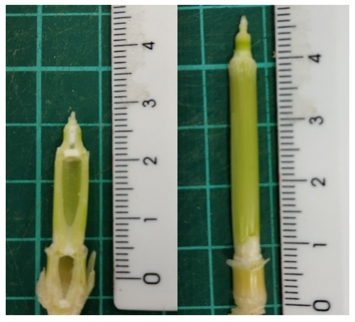
2.3. Anatomical Observation

Destructive sampling was conducted weekly from the maximum tillering stage until the flag leaf collar formation stage (Figure 1). Three pots of plants were randomly selected and sent to the laboratory for dissection. All culms of the plants were dissected for anatomical observation. A culm containing either green-ring or 1–3 mm panicle is considered as a reproductive culm (Figure 2). The beginning of the reproductive phase is defined when the proportion of reproductive culm has reached 50%.

2.4. Plant Traits Examination

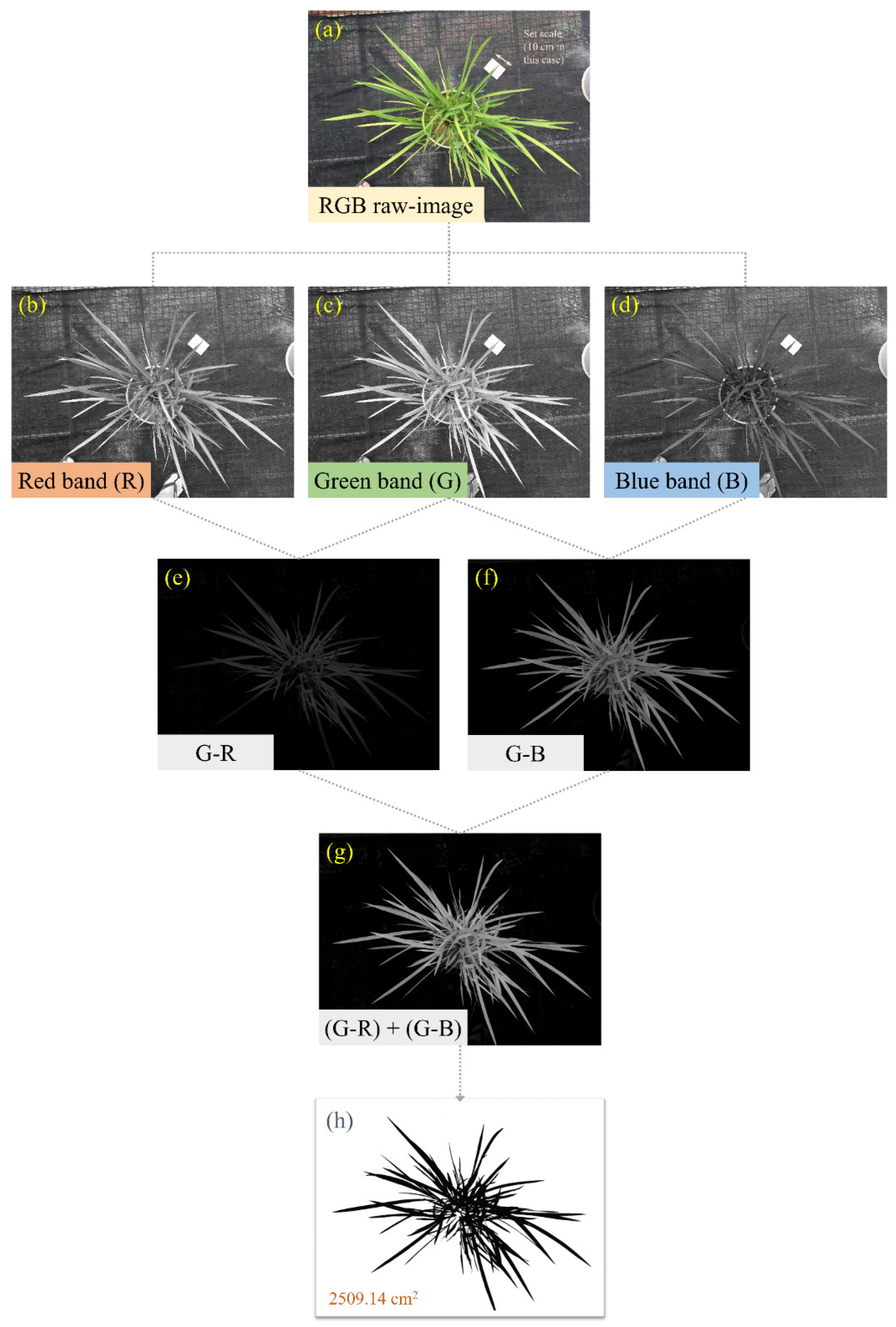
2.4.1. Leaf Cover Area (LCA)

Before destructive sampling, leaf cover area (LCA) and leaf chlorophyll content were measured. The LCA measurement, which is an uncommon method for leaf area-related ground-truth observation, was done with a smartphone-RGB camera and ImageJ software (version 1.53) (National Institutes of Health, Bethesda, MD, USA). The procedure was graphically illustrated in Figure 3. A white panel was placed beside the target plant as a reference length for subsequent image analysis. Then, an RGB-image was taken with a smartphone-RGB camera that was held vertically and approximately one meter above the soil surface. Subsequently, the captured image was loaded into the ImageJ software for LCA estimation. Firstly, a straight line was drawn according to the border of the white panel within the raw image, and a known-scale was set to define the pixel unit to distance unit (Figure 3a). Secondly, the image was converted to 8-bit RGB color channels (Figure 3b–d). Then, the 8-bit images were transformed by the equation (G − R) + (G − B) to extract the plant pixels (Figure 3e–g). It is worth noting that, since the default image data type of the software is uint8, rearranging the formula might be unwise. For example, (G + G) − (R + B) could yield different results, although it is mathematically equivalent to the (G − R) + (G − B). Lastly, the plant pixels were masked out by Otsu thresholding, and finally the LCA was estimated (Figure 3h).

2.4.2. Leaf Chlorophyll Content (SPAD)

The leaf chlorophyll content was investigated with a chlorophyll meter (Chlorophyll meter SPAD-502Plus, Konica Minolta, Tokyo, Japan). The SPAD measurements were made at the 2/3 position on the third fully expanded leaf from the top [38].

2.4.3. Leaf Dry Weight (LDW), N Content (LNC), and N Accumulation (LNA)
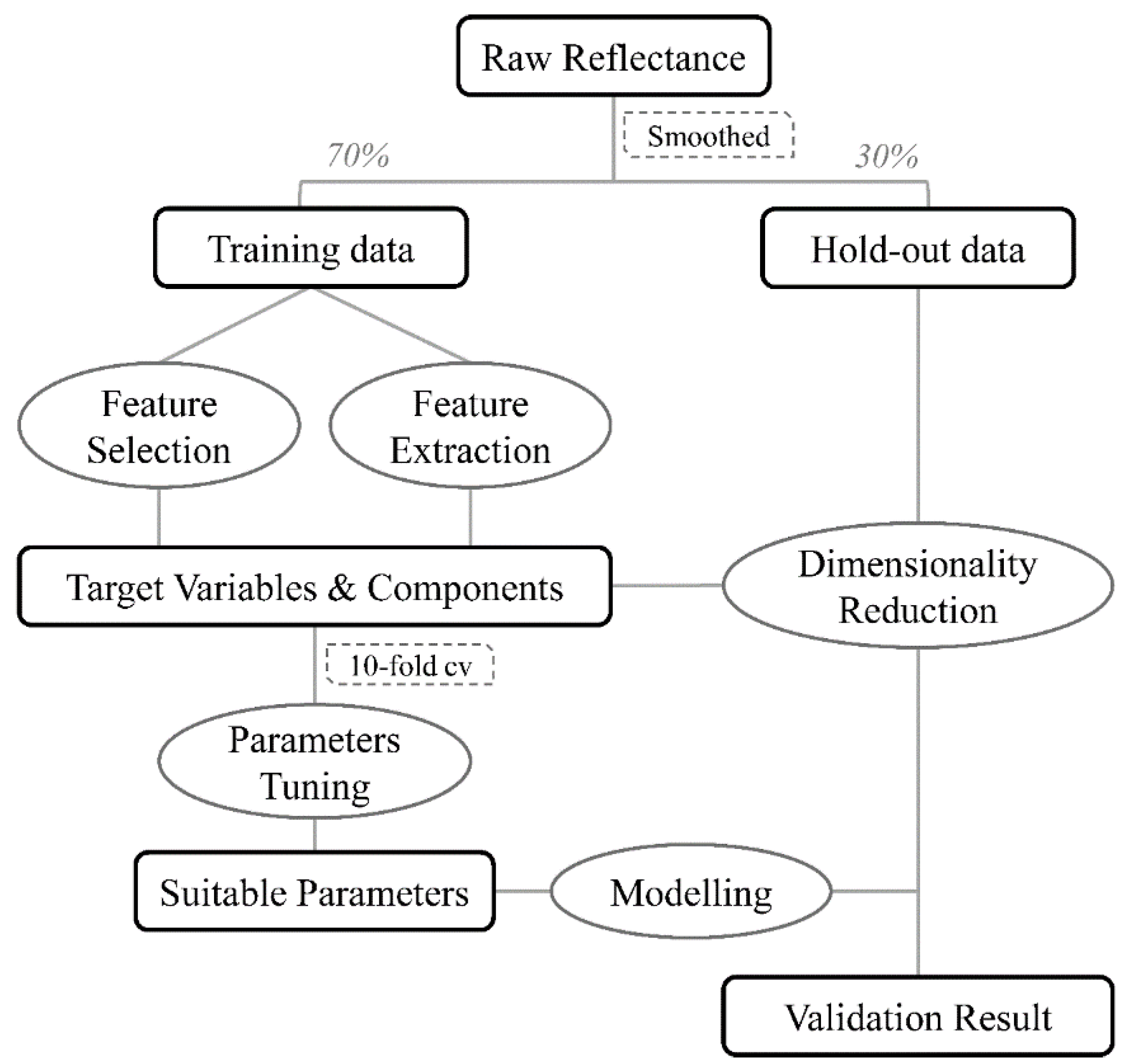
After dissection for anatomical observation, the leaves were oven-dried until constant weight at 80 °C to obtain the leaf dry weight (LDW). The leaf N content (LNC) was determined by the Kjeldahl method. The leaf nitrogen accumulation (LNA) was calculated by multiplying LDW with LNC, where:
LNA = LDW × LNC

2.5. Data Analysis

The data analysis was implemented in R software (version 4.1.0) [39]. The procedure is illustrated in Figure 4.

2.5.1. Data Pretreatment and Partition

The raw spectral data were smoothed before subsequent analysis [33]. As a result, the smoothed spectral data for subsequent analysis ranged from 327 nm to 1073 nm. Next, the smoothed data were randomly partitioned into two parts: 70% as the training dataset, and the remaining were held out for validation.

2.5.2. Dimensionality Reduction

Two dimensionality-reduction techniques, FE and FS approaches, were applied on the smoothed hyperspectral data. The FE approach was performed with PCA. The eigenvalues of each component were calculated with a correlation matrix. Subsequently, a suitable number of principal components (PCs) were determined according to the proportion of variance explained (PVE) in the scree-plot. The extracted features were then used to establish logistic regression (FE-logistic), RF (FE-RF), and SVM (FE-SVM) models.
On the other hand, the FS approach was performed with RF. Several wavelengths were selected according to the variable importance that was measured with the Gini index. The selected wavelengths were then used to construct logistic regression (FS-logistic), RF (FS-RF), and SVM (FS-SVM) models.

2.5.3. Parameters Tuning

The parameters of each algorithm were tuned in a 10-fold cross-validation procedure. The optimal cutoff threshold of logistic regression was determined as the cross-point of sensitivity and specificity [40]. The number of trees (ntree), the number of variables (mtry) of RF, and the cost and gamma of SVM (RBF kernel) were decided based on the highest accuracy obtained in the grid search method. The fine-tuned parameters were then applied to internal data modelling (Table 1) and consequently validated by the hold-out dataset.

2.5.4. Model Performance Evaluation

A confusion matrix was adopted to deal with binary classification purposes (Table 2). Subsequently, four metrics derived from the confusion matrix were used to evaluate the performance of each classifier.
The derivatives are expressed as follows:
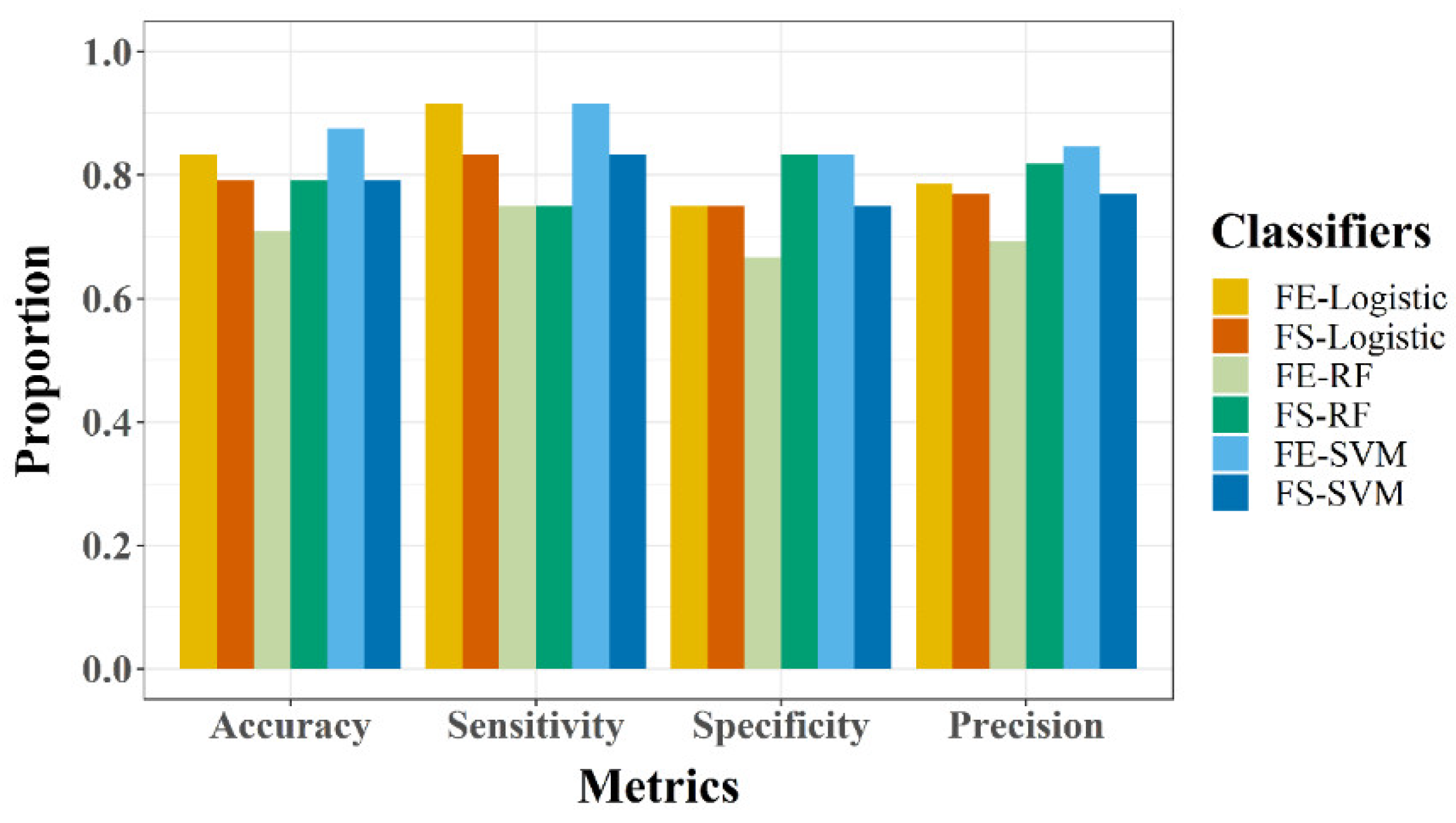
  • Accuracy: This represents an overall proportion of accurate classification (correctly classified vegetative and reproductive, respectively).
Accuracy = TP + TN TP + TN + FP + FN
  • Sensitivity: This shows how well the classifiers can identify the reproductive phase when the rice plant enters the reproductive phase.
Sensitivity = TP TP + FN
  • Specificity: This shows how well the classifiers can identify vegetative phase when the rice plant has not entered reproductive phase.
Specificity = TN TN + FP
  • Precision: This computes the probability that a positive prediction is accurate.
Precision = TP TP + FP

3. Results and Discussion

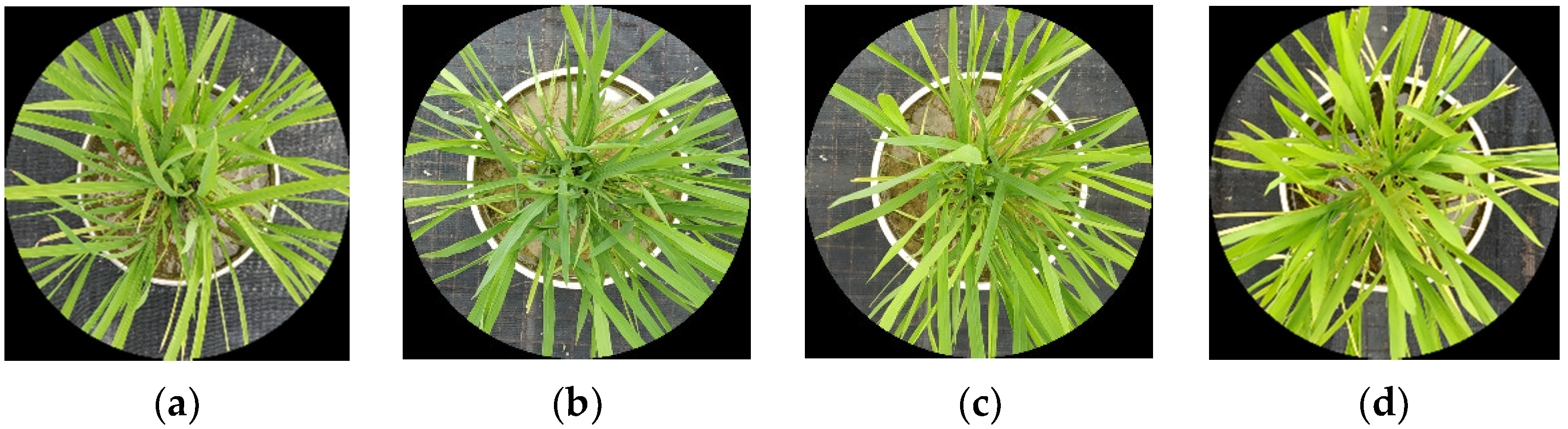
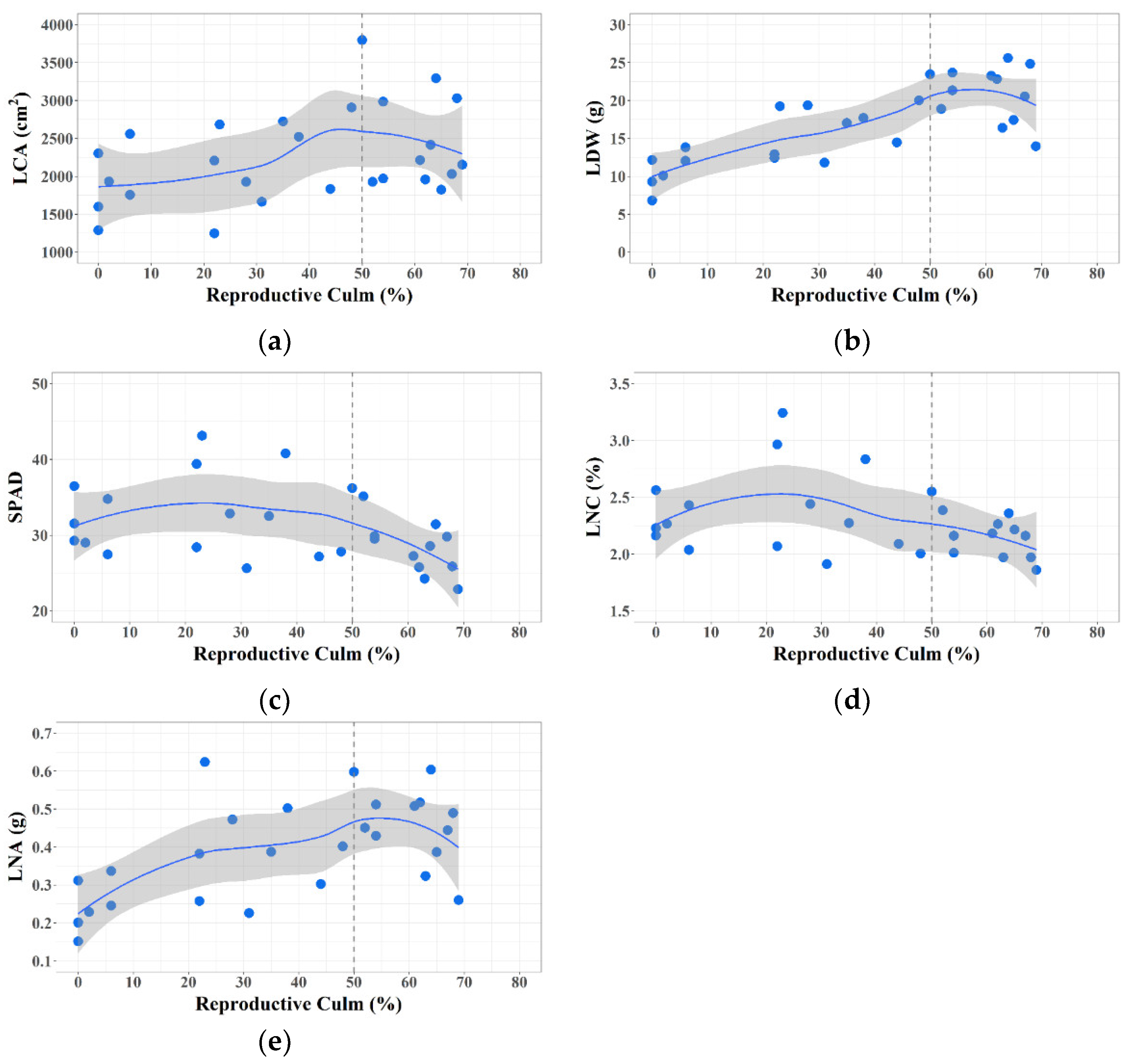
3.1. Plant Trait Changes during Phase Transition

The LCA progressively expanded during LV and reached maxima before ER (Figure 5a). This might have resulted from the decrease in leaf area and leaf length after panicle initiation [29]. At the same time, the LDW gradually increased before ER and started to decline after LV (Figure 5b). This revealed that the leaf biomass accumulation was retarded after the transition to ER.
On the other hand, the dynamic changes of SPAD values represented the color changes of the leaves during phase transition (Figure 5c). The SPAD values in LV were higher than those in ER, depicting the color of leaves turned from green to yellowish-green during phase transition. The reason is generally related to the degradation of chlorophyll that is a common phenomenon during leaf senescence. Besides, LNC declined during ER regardless of the decrement in LDW (Figure 5d). The result indicated that the process of N translocation from leaf (source) to stem (sink) had synchronously occurred along with chlorophyll degradation. The N requirement of the panicle is continuously elevated after the transition to ER, while the plant total N absorption declines after the vegetative phase’s end [41]. Consequently, N is translocated from leaves to panicles to compensate for the demand of panicle development. The N translocation process is especially obvious when N supply is inefficient during ER [10]. The reduction in LNA during ER further revealed the N translocation process (Figure 5e).
In summary, three symptoms indicate the transition from LV to ER. First, the coverage is maximally extended before ER; second, the leaf growth is retarded after LV; and third, the leaves appear from green to yellowish-green due to N translocation.

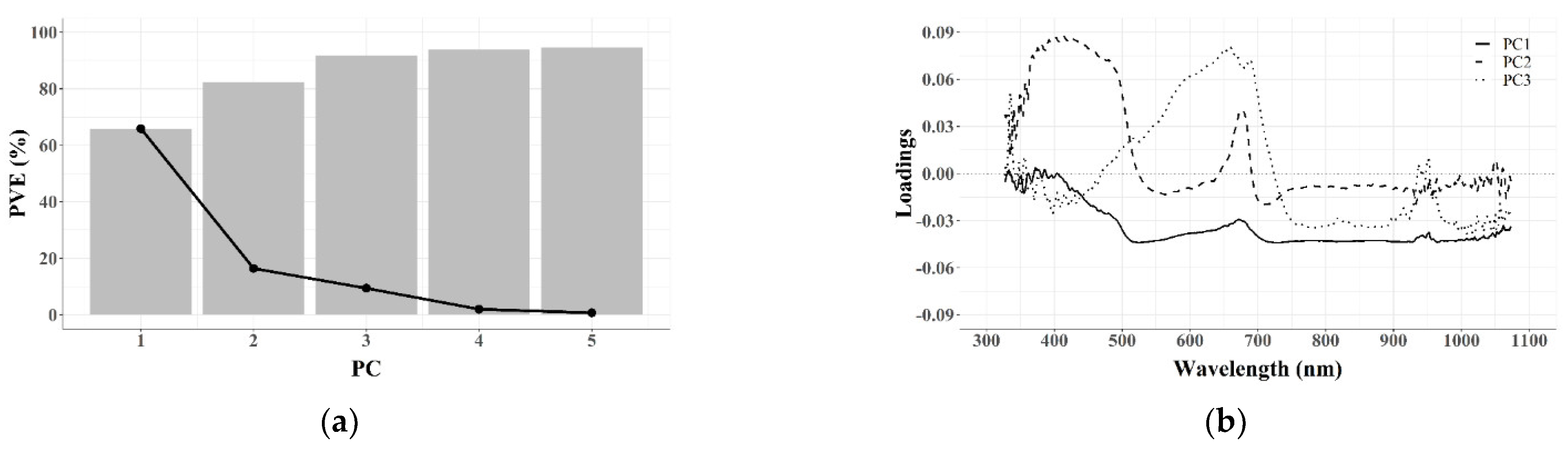
3.2. Dimensionality Reduction

3.2.1. Feature Extraction (FE)

The FE-based dimensionality reduction was done with the PCA algorithm according to the proportion of variance explained (PVE) of each principal component (PC). The result showed that the former five PCs explained 65.93%, 16.45%, 9.43%, 2.00%, and 0.74% of the data variances, respectively (Figure 6a). The scree-plot’s elbow bent on PC2; however, PC3 was also taken into consideration to achieve an over 90% cumulative PVE [33]. The contributions of each wavelength to the extracted PCs were further represented with a loadings plot (Figure 6b).
The major contents of PC1 could be roughly separated into three parts according to the peaks of eigenvectors and are the green region (500–600 nm), the red-edge region (680–750 nm), and the NIR region (>750 nm). The trough around 510–540 nm involved pigment variation (chlorophyll, carotenoids, and anthocyanin) [42,43,44] and the xanthophyll signal [45]. The result indicates PC1 might be a physiological indicator. However, the PC1 subsequently inflected on the red-edge region (around 675 nm) and appeared as a basin throughout the red-edge and NIR regions. The red-edge region is comprehensive in plant monitoring and is related to the plant’s structural and physiological status, such as leaf area index (LAI) and chlorophyll content [46]. Besides, the NIR region correlates with biophysical changes such as intra- and inter-cellular properties, leaf orientation, and plant coverage [47,48]. Due to the confounding effects of PC1, it is rather difficult, if not impossible, to be interpreted as a single or several plant traits.
The PC2 provoked a major peak in the blue region (350–450 nm) and a short peak in the red region (670–680 nm) (Figure 6b). The blue region is related to plant pigment absorption, which provides much information on plant physiological status and indicates the phenological stage [49]. Meanwhile, chlorophyll absorbs strongly in the red region, with maximum absorbance between 660 and 680 nm. These led the PC2 to be assumed as a physiological feature. However, the correlation of PC2 with physiological measurements (SPAD, LNC, and LNA) in this work was insignificant. The reason might be due to the overlapping absorption features of major pigments and other constituents [49,50,51]. Furthermore, the wavelengths around 675 nm were suggested to be insensitive to pigment variation unless the chlorophyll content is very low [52]. On the other hand, this work suggested that PC2 was negatively correlated with LCA to some extent (r = −0.373; p < 0.09) (Table 3). The negative correlation between PC2 and LCA was reasonable, as the extension of LCA would probably increase the area of blue light absorption, thus reducing blue light reflectance. Hence, PC2 could be partly considered as a physical feature rather than a physiological feature.
PC3 mainly constituted the red and red-edge regions (Figure 6b). Preceding studies showed that several wavelengths within the red and red-edge region correlate with N content [32,53]. However, the correlation between PC3 and LNC was rather insignificant in this work. The reason might be the impact of considerable loadings from the NIR region that is insensitive to chlorophyll and thus N content [47,54]. Nonetheless, PC3 negatively correlated with LNA (r = −0.440; p < 0.05). The LNA depicts the growth amount of plants, particularly the enrichment of nitrogen and carbon. Besides, the insignificant correlation between PC3 and LCA is reasonable, as previous research proved that the red-edge region is unaffected by ground cover [46]. On the whole, PC3 tended to be a physiological feature due to the stronger correlation with LNA.

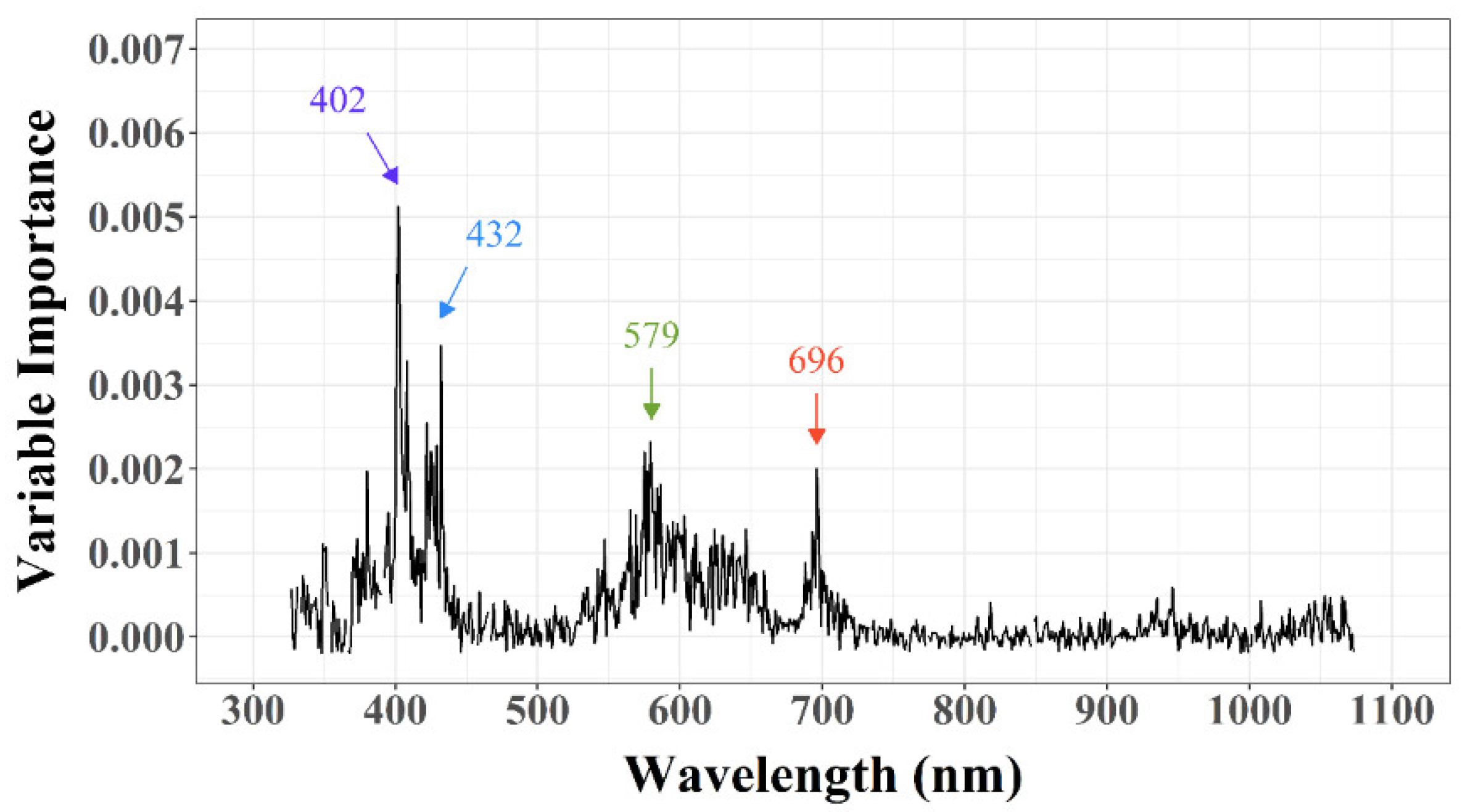
3.2.2. Feature Selection (FS)

The FS-based dimensionality reduction was performed with a random forest (RF) algorithm. The importance of each wavelength was measured with permutation accuracy. Figure 7 represents four groups of peaks that are located within blue (350–450 nm), blue-green edge (450–499 nm), green (500–600 nm), and red-edge (680–750 nm) regions. Considering the problem of data collinearity, only a single representative wavelength would be selected from each region. Consequently, 402, 432, 579, and 696 nm were selected for subsequent modeling.
Although major plant pigments absorb blue wavelengths, their strong absorbance peak is above 430 nm, which is quite far from 402 nm [49]. Meanwhile, the wavelengths around 402 nm were of lesser concern. Interestingly, 402 nm was also one of the highest loadings of PC2 in the previous section. The result showed that 402 nm negatively correlated with LCA to some extent (p < 0.09) (Table 4). The weak correlation between LCA and either PC2 or 402 nm might be caused by the insufficient area of the detection spot. The detection spot could be enlarged by elevating the detector’s height; however, it is rather difficult to achieve due to the observer’s height limitation. On the contrary, 432 nm is very near 430 nm, one of the main absorption peaks of carotenoids [43]. The 432 nm wavelength probably correlated with carotenoid content and could be an indicator of leaf senescence.
On the other hand, 579 nm is intuitively a yellow wavelength representing the plant’s yellowness. Although the carotenoids are the principal pigments that correspond to the yellowish appearance of leaves, the correlation between 579 nm and carotenoid content might be indirect. Preceding research found that those wavelengths above 550 nm within the green region are only governed by chlorophyll absorption [43]. Therefore, the yellowness of leaf appearance during phase transition was probably caused by the degradation of chlorophyll. Table 4 represents the significant correlation of 579 nm with SPAD and LNC (p < 0.001).
Besides, 696 nm within the range of 690–705 nm could be a sensitive indicator of chlorophyll content [50]. Furthermore, several studies also stated that 696 nm correlates with chlorophyll content and N content [55,56]. The situations were also similar, as shown in the results, that 696 nm had significant correlation with SPAD (p < 0.001), LNC (p < 0.001), and LNA (p < 0.05).

3.3. Model Evaluation

In order to construct the predicted model, the extracted features (PC1, PC2, and PC3) and selected features (402, 432, 579, and 696 nm) were applied for modelling and comparing the performances. Four metrics evaluated the constructed models: accuracy, sensitivity, specificity, and precision, as shown in Figure 8. The FE-logistic (accuracy = 0.833) and FE-SVM (accuracy = 0.875) represented a higher overall proportion of correct classification. Besides, the FE-logistic (sensitivity = 0.917) and FE-SVM (sensitivity = 0.917) exhibited greater ability for recognizing the ER. On the contrary, the FS-RF (specificity = 0.833) and FE-SVM (specificity = 0.833) showed better performance in identifying the LV. Nonetheless, the FE-SVM (precision = 0.846) and FS-RF (precision = 0.818) manifested higher reliability of positive estimation.
The performance of the FE-logistic was comparable to the FE-SVM to some extent if considering the computational cost. However, the lower precision indicated the FE-logistic could be somewhat over-sensitive. An over-sensitive model would easily misclassify the LV as ER and consequently mislead N application at LV. When a cultivar with high lodging resistance is planted, the FE-logistic could be a competent model. On the contrary, the FE-SVM is more appropriate for general application.

4. Conclusions

This study represented the workflow of hyperspectral sensing for the discrimination of rice late vegetative phase (LV) and early reproductive phase (ER). Moreover, the physical and physiological changes of the rice plant during phase transition were also illustrated. Furthermore, the realistic implications of the spectral features were inferenced. As shown in the experimental results, the leaf cover area (LCA), leaf dry weight (LDW), and leaf N accumulation (LNA) of rice plants progressively increased, while the chlorophyll content (SPAD) and leaf nitrogen content (LNC) remained stable during LV. After reaching ER, the N translocation from leaves to emerging panicles led to chlorophyll degradation. Although these differences were obscure to human observation, hyperspectral sensing could still distinguish the differences in a non-destructive and high-temporal-resolution manner. Considering the detrimental effect of applying N at LV, the feature extraction-based support vector machine (FE-SVM) was suggested for the timing assessment of panicle fertilizer application. Further effort is still required to integrate this timing assessment approach with extensively published nitrogen status monitoring techniques for precise N management.

Author Contributions

Conceptualization, J.-K.L. and W.-S.L.; Investigation, J.-K.L.; Methodology, J.-K.L.; Visualization, J.-K.L.; Writing—original draft, J.-K.L.; Writing—review and editing, J.-K.L. and W.-S.L.; Resources, W.-S.L.; Funding acquisition, W.-S.L. All authors have read and agreed to the published version of the manuscript.

Funding

This research was partially funded by the Ministry of Science and Technology (MOST), Taiwan (grant number MOST 110-2637-B-020-005).

Institutional Review Board Statement

Not applicable.

Informed Consent Statement

Not applicable.

Data Availability Statement

Not applicable.

Acknowledgments

The authors wish to thank Kuan-Hui Lin, Tai-Hsin Lin, Sung-Yu Yang, Ya-Hui Liu, En-Yu Lu and Zi-You Lin for their assistance in the laboratory experiments and study site maintenance in this study. The authors also want to thank Chih-Sheng Sheu, who retired from the Taichung District Agricultural Research and Extension Station, COA, for sharing the rice planting experience.

Conflicts of Interest

The authors declare no conflict of interest.

References

  1. Fahad, S.; Adnan, M.; Noor, M.; Arif, M.; Alam, M.; Khan, I.A.; Ullah, H.; Wahid, F.; Mian, I.A.; Jamal, Y.; et al. Chapter 1—Major constraints for global rice production. In Advances in Rice Research for Abiotic Stress Tolerance; Hasanuzzaman, M., Fujita, M., Nahar, K., Biswas, J.K., Eds.; Woodhead Publishing: Sawston, UK, 2019; pp. 1–22. ISBN 978-0-12-814332-2. [Google Scholar]
  2. Fageria, N.K.; Baligar, V.C. Yield and Yield Components of Lowland Rice as Influenced by Timing of Nitrogen Fertilization. J. Plant Nutr. 1999, 22, 23–32. [Google Scholar] [CrossRef]
  3. Kamiji, Y.; Yoshida, H.; Palta, J.A.; Sakuratani, T.; Shiraiwa, T. N Applications That Increase Plant N during Panicle Development Are Highly Effective in Increasing Spikelet Number in Rice. Field Crop. Res. 2011, 122, 242–247. [Google Scholar] [CrossRef]
  4. Zhou, W.; Lv, T.; Yang, Z.; Wang, T.; Fu, Y.; Chen, Y.; Hu, B.; Ren, W. Morphophysiological Mechanism of Rice Yield Increase in Response to Optimized Nitrogen Management. Sci. Rep. 2017, 7, 17226. [Google Scholar] [CrossRef] [PubMed] [Green Version]
  5. Ju, C.; Zhu, Y.; Liu, T.; Sun, C. The Effect of Nitrogen Reduction at Different Stages on Grain Yield and Nitrogen Use Efficiency for Nitrogen Efficient Rice Varieties. Agronomy 2021, 11, 462. [Google Scholar] [CrossRef]
  6. Ju, C.; Liu, T.; Sun, C. Panicle Nitrogen Strategies for Nitrogen-Efficient Rice Varieties at a Moderate Nitrogen Application Rate in the Lower Reaches of the Yangtze River, China. Agronomy 2021, 11, 192. [Google Scholar] [CrossRef]
  7. Counce, P.A.; Keisling, T.C.; Mitchell, A.J. A Uniform, Objective, and Adaptive System for Expressing Rice Development. Crop Sci. 2000, 40, 436–443. [Google Scholar] [CrossRef] [Green Version]
  8. Muhammad, S.; Kim, U.J.; Kumazawa, K. The Uptake, Distribution, and Accumulation of 15N-Labelled Ammonium and Nitrate Nitrogen Top-Dressed at Different Growth Stages of Rice. Soil Sci. Plant Nutr. 1974, 20, 279–286. [Google Scholar] [CrossRef]
  9. Zhou, W.; Yang, Z.; Wang, T.; Fu, Y.; Chen, Y.; Hu, B.; Yamagishi, J.; Ren, W. Environmental Compensation Effect and Synergistic Mechanism of Optimized Nitrogen Management Increasing Nitrogen Use Efficiency in Indica Hybrid Rice. Front. Plant Sci. 2019, 10, 245. [Google Scholar] [CrossRef]
  10. Peng, S.; Cassman, K.G. Upper Thresholds of Nitrogen Uptake Rates and Associated Nitrogen Fertilizer Efficiencies in Irrigated Rice. Agron. J. 1998, 90, 178–185. [Google Scholar] [CrossRef]
  11. Wang, Z.; Zhang, F.; Xiao, F.; Tao, Y.; Liu, Z.; Li, G.; Wang, S.; Ding, Y. Contribution of Mineral Nutrients from Source to Sink Organs in Rice under Different Nitrogen Fertilization. Plant Growth Regul. 2018, 86, 159–167. [Google Scholar] [CrossRef] [Green Version]
  12. Quang Duy, P.; Abe, A.; Hirano, M.; Sagawa, S.; Kuroda, E. Analysis of Lodging-Resistant Characteristics of Different Rice Genotypes Grown under the Standard and Nitrogen-Free Basal Dressing Accompanied with Sparse Planting Density Practices. Plant Prod. Sci. 2004, 7, 243–251. [Google Scholar] [CrossRef]
  13. Pan, J.; Zhao, J.; Liu, Y.; Huang, N.; Tian, K.; Shah, F.; Liang, K.; Zhong, X.; Liu, B. Optimized Nitrogen Management Enhances Lodging Resistance of Rice and Its Morpho-Anatomical, Mechanical, and Molecular Mechanisms. Sci. Rep. 2019, 9, 20274. [Google Scholar] [CrossRef] [PubMed] [Green Version]
  14. Liu, Y.; Zhu, X.; He, X.; Li, C.; Chang, T.; Chang, S.; Zhang, H.; Zhang, Y. Scheduling of Nitrogen Fertilizer Topdressing during Panicle Differentiation to Improve Grain Yield of Rice with a Long Growth Duration. Sci. Rep. 2020, 10, 15197. [Google Scholar] [CrossRef] [PubMed]
  15. Moldenhauer, K.; Counce, P.; Hardke, J. Rice growth and development. In Rice Production Handbook; Hardke, J., Ed.; University of Arkansas Division of Agriculture: Little Rock, AR, USA, 2001; Volume 192, pp. 7–14. [Google Scholar]
  16. Dunand, R.; Saichuk, J. Rice growth and development. In Louisiana Rice Production Handbook; Saichuk, J., Ed.; Louisiana State University Agricultural Center: Baton Rouge, LA, USA, 2014; Volume 2321, pp. 41–53. [Google Scholar]
  17. Gilmore, E.C.; Rogers, J.S. Heat Units as a Method of Measuring Maturity in Corn 1. Agron. J. 1958, 50, 611–615. [Google Scholar] [CrossRef]
  18. Aslam, M.A.; Ahmed, M.; Stöckle, C.O.; Higgins, S.S.; Hayat, R. Can Growing Degree Days and Photoperiod Predict Spring Wheat Phenology? Front. Environ. Sci. 2017, 5, 57. [Google Scholar] [CrossRef]
  19. Bonhomme, R. Bases and limits to using ‘degree.day’ units. Eur. J. Agron. 2000, 13, 1–10. [Google Scholar] [CrossRef]
  20. Zeng, L.; Wardlow, B.D.; Xiang, D.; Hu, S.; Li, D. A Review of Vegetation Phenological Metrics Extraction Using Time-Series, Multispectral Satellite Data. Remote Sens. Environ. 2020, 237, 111511. [Google Scholar] [CrossRef]
  21. Yang, Q.; Shi, L.; Han, J.; Yu, J.; Huang, K. A Near Real-Time Deep Learning Approach for Detecting Rice Phenology Based on UAV Images. Agric. For. Meteorol. 2020, 287, 107938. [Google Scholar] [CrossRef]
  22. Zheng, H.; Cheng, T.; Yao, X.; Deng, X.; Tian, Y.; Cao, W.; Zhu, Y. Detection of Rice Phenology through Time Series Analysis of Ground-Based Spectral Index Data. Field Crop. Res. 2016, 198, 131–139. [Google Scholar] [CrossRef]
  23. Hufkens, K.; Melaas, E.K.; Mann, M.L.; Foster, T.; Ceballos, F.; Robles, M.; Kramer, B. Monitoring Crop Phenology Using a Smartphone Based Near-Surface Remote Sensing Approach. Agric. For. Meteorol. 2019, 265, 327–337. [Google Scholar] [CrossRef]
  24. Guo, L.; An, N.; Wang, K. Reconciling the Discrepancy in Ground-and Satellite-observed Trends in the Spring Phenology of Winter Wheat in China from 1993 to 2008. J. Geophys. Res. Atmos. 2016, 121, 1027–1042. [Google Scholar] [CrossRef] [Green Version]
  25. Zhou, M.; Ma, X.; Wang, K.; Cheng, T.; Tian, Y.; Wang, J.; Zhu, Y.; Hu, Y.; Niu, Q.; Gui, L. Detection of Phenology Using an Improved Shape Model on Time-Series Vegetation Index in Wheat. Comput. Electron. Agric. 2020, 173, 105398. [Google Scholar] [CrossRef]
  26. Guo, W.; Fukatsu, T.; Ninomiya, S. Automated Characterization of Flowering Dynamics in Rice Using Field-Acquired Time-Series RGB Images. Plant Methods 2015, 11, 1–14. [Google Scholar] [CrossRef] [PubMed] [Green Version]
  27. Zhu, Y.; Cao, Z.; Lu, H.; Li, Y.; Xiao, Y. In-Field Automatic Observation of Wheat Heading Stage Using Computer Vision. Biosyst. Eng. 2016, 143, 28–41. [Google Scholar] [CrossRef]
  28. Bai, X.; Cao, Z.; Zhao, L.; Zhang, J.; Lv, C.; Li, C.; Xie, J. Rice Heading Stage Automatic Observation by Multi-Classifier Cascade Based Rice Spike Detection Method. Agric. For. Meteorol. 2018, 259, 260–270. [Google Scholar] [CrossRef]
  29. Tivet, F.; Pinheiro, B.D.S.; Raïssac, M.D.; Dingkuhn, M. Leaf Blade Dimensions of Rice (Oryza sativa L. and Oryza glaberrima Steud.). Relationships between Tillers and the Main Stem. Ann. Bot. 2001, 88, 507–511. [Google Scholar] [CrossRef]
  30. Xu, X.; Liang, T.; Zhu, J.; Zheng, D.; Sun, T. Review of Classical Dimensionality Reduction and Sample Selection Methods for Large-Scale Data Processing. Neurocomputing 2019, 328, 5–15. [Google Scholar] [CrossRef]
  31. Asner, G.P. Biophysical and Biochemical Sources of Variability in Canopy Reflectance. Remote Sens. Environ. 1998, 64, 234–253. [Google Scholar] [CrossRef]
  32. Song, S.; Gong, W.; Zhu, B.; Huang, X. Wavelength Selection and Spectral Discrimination for Paddy Rice, with Laboratory Measurements of Hyperspectral Leaf Reflectance. ISPRS J. Photogramm. Remote Sens. 2011, 66, 672–682. [Google Scholar] [CrossRef]
  33. Liu, Z.-Y.; Qi, J.-G.; Wang, N.-N.; Zhu, Z.-R.; Luo, J.; Liu, L.-J.; Tang, J.; Cheng, J.-A. Hyperspectral Discrimination of Foliar Biotic Damages in Rice Using Principal Component Analysis and Probabilistic Neural Network. Precis. Agric. 2018, 19, 973–991. [Google Scholar] [CrossRef]
  34. Almeida, T.I.R.; Filho, D.S. Principal Component Analysis Applied to Feature-Oriented Band Ratios of Hyperspectral Data: A Tool for Vegetation Studies. Int. J. Remote Sens. 2004, 25, 5005–5023. [Google Scholar] [CrossRef]
  35. Breiman, L. Random Forests. Mach. Learn. 2001, 45, 5–32. [Google Scholar] [CrossRef] [Green Version]
  36. Liaw, A.; Wiener, M. Classification and Regression by RandomForest. R News 2002, 2, 18–22. [Google Scholar]
  37. Abdel-Rahman, E.M.; Ahmed, F.B.; Ismail, R. Random Forest Regression and Spectral Band Selection for Estimating Sugarcane Leaf Nitrogen Concentration Using EO-1 Hyperion Hyperspectral Data. Int. J. Remote Sens. 2013, 34, 712–728. [Google Scholar] [CrossRef]
  38. Yuan, Z.; Cao, Q.; Zhang, K.; Ata-Ul-Karim, S.T.; Tian, Y.; Zhu, Y.; Cao, W.; Liu, X. Optimal Leaf Positions for SPAD Meter Measurement in Rice. Front. Plant Sci. 2016, 7, 719. [Google Scholar] [CrossRef] [Green Version]
  39. R Core Team. R: A Language and Environment for Statistical Computing; R Foundation for Statistical Computing: Vienna, Austria, 2021; Available online: https://www.R-project.org (accessed on 18 May 2021).
  40. Peng, C.-Y.J.; So, T.-S.H. Logistic Regression Analysis and Reporting: A Primer. Underst. Stat. Stat. Issues Psychol. Educ. Soc. Sci. 2002, 1, 31–70. [Google Scholar] [CrossRef]
  41. Sheehy, J.E.; Mnzava, M.; Cassman, K.G.; Mitchell, P.L.; Pablico, P.; Robles, R.P.; Samonte, H.P.; Lales, J.S.; Ferrer, A.B. Temporal Origin of Nitrogen in the Grain of Irrigated Rice in the Dry Season: The Outcome of Uptake, Cycling, Senescence and Competition Studied Using a 15N-Point Placement Technique. Field Crop. Res. 2004, 89, 337–348. [Google Scholar] [CrossRef]
  42. Zur, Y.; Gitelson, A.A.; Chivkunova, O.B.; Merzlyak, M.N. The Spectral Contribution of Carotenoids to Light Absorption and Reflectance in Green Leaves. In Proceedings of the 2nd International Conference Geospatial Information in Agriculture and Forestry, Buena Vista, FL, USA, 10–12 January 2000; Volume 2. [Google Scholar]
  43. Gitelson, A.A.; Zur, Y.; Chivkunova, O.B.; Merzlyak, M.N. Assessing Carotenoid Content in Plant Leaves with Reflectance Spectroscopy. Photochem. Photobiol. 2002, 75, 272–281. [Google Scholar] [CrossRef]
  44. Merzlyak, M.N.; Solovchenko, A.E.; Gitelson, A.A. Reflectance Spectral Features and Non-Destructive Estimation of Chlorophyll, Carotenoid and Anthocyanin Content in Apple Fruit. Postharvest Biol. Technol. 2003, 27, 197–211. [Google Scholar] [CrossRef]
  45. Gamon, J.A.; Penuelas, J.; Field, C.B. A Narrow-Waveband Spectral Index That Tracks Diurnal Changes in Photosynthetic Efficiency. Remote Sens. Environ. 1992, 41, 35–44. [Google Scholar] [CrossRef]
  46. Horler, D.N.H.; Dockray, M.; Barber, J. The Red Edge of Plant Leaf Reflectance. Int. J. Remote Sens. 1983, 4, 273–288. [Google Scholar] [CrossRef]
  47. Knipling, E.B. Physical and Physiological Basis for the Reflectance of Visible and Near-Infrared Radiation from Vegetation. Remote Sens. Environ. 1970, 1, 155–159. [Google Scholar] [CrossRef]
  48. Woolley, J.T. Reflectance and Transmittance of Light by Leaves. Plant Physiol. 1971, 47, 656–662. [Google Scholar] [CrossRef] [PubMed] [Green Version]
  49. Blackburn, G.A. Hyperspectral Remote Sensing of Plant Pigments. J. Exp. Bot. 2007, 58, 855–867. [Google Scholar] [CrossRef] [Green Version]
  50. Gitelson, A.A.; Merzlyak, M.N. Signature Analysis of Leaf Reflectance Spectra: Algorithm Development for Remote Sensing of Chlorophyll. J. Plant Physiol. 1996, 148, 494–500. [Google Scholar] [CrossRef]
  51. Sims, D.A.; Gamon, J.A. Relationships between Leaf Pigment Content and Spectral Reflectance across a Wide Range of Species, Leaf Structures and Developmental Stages. Remote Sens. Environ. 2002, 81, 337–354. [Google Scholar] [CrossRef]
  52. Gitelson, A.; Merzlyak, M.N. Spectral Reflectance Changes Associated with Autumn Senescence of Aesculus Hippocastanum, L. and Acer Platanoides, L. Leaves. Spectral Features and Relation to Chlorophyll Estimation. J. Plant Physiol. 1994, 143, 286–292. [Google Scholar] [CrossRef]
  53. Mahajan, G.R.; Pandey, R.N.; Sahoo, R.N.; Gupta, V.K.; Datta, S.C.; Kumar, D. Monitoring Nitrogen, Phosphorus and Sulphur in Hybrid Rice (Oryza sativa L.) Using Hyperspectral Remote Sensing. Precis. Agric. 2017, 18, 736–761. [Google Scholar] [CrossRef]
  54. Wada, S.; Hayashida, Y.; Izumi, M.; Kurusu, T.; Hanamata, S.; Kanno, K.; Kojima, S.; Yamaya, T.; Kuchitsu, K.; Makino, A. Autophagy Supports Biomass Production and Nitrogen Use Efficiency at the Vegetative Stage in Rice. Plant Physiol. 2015, 168, 60–73. [Google Scholar] [CrossRef] [PubMed] [Green Version]
  55. Tkachuk, R.; Mellish, V.J.; Daun, J.K.; Macri, L.J. Determination of Chlorophyll in Ground Rapeseed Using a Modified near Infrared Reflectance Spectrophotometer. J. Am. Oil Chem. Soc. 1988, 65, 381–385. [Google Scholar] [CrossRef]
  56. Dedeoglu, M. Estimation of Critical Nitrogen Contents in Peach Orchards Using Visible-near Infrared Spectral Mixture Analysis. J. Infrared Spectrosc. 2020, 28, 315–327. [Google Scholar] [CrossRef]
Figure 1. Illustration of rice LV, which includes (a) maximum tillering stage and (b) vegetative-lag stage; and ER, which consists of (c) panicle initiation stage and (d) flag leaf collar formation stage. This figure is a rough simulation of the spectroradiometer’s detection spot instead of the real instrumental view.
Agronomy 11 02465 g001
Figure 2. Anatomical observation of first internode-elongation during LV (left); and green-ring with a 1–3 mm panicle during ER (right).
Agronomy 11 02465 g002
Figure 3. Illustration of leaf cover area (LCA) estimation procedure. (a) Define the drawn pixels unit; (bd) split channel; (eg) transformation with (G − R) + (G − B) formula; (h) estimating the threshold area.
Agronomy 11 02465 g003
Figure 4. Illustration of the data analysis procedure.
Agronomy 11 02465 g004
Figure 5. Illustration of (a) leaf cover area (LCA), (b) leaf dry weight (LDW), (c) chlorophyll meter readings (SPAD), (d) leaf N content (LNC), and (e) leaf N accumulation (LNA). The grey-dashed vertical line denotes the beginning of the reproductive phase.
Agronomy 11 02465 g005
Figure 6. Feature extraction is based on (a) the proportion of variance explained (PVE) (black dots and line) and cumulative PVE (grey bars) of each principal component (PC). The variable importance was depicted by (b) the loadings plot that consists of the eigenvectors of the PC1 (solid line), PC2 (dashed line), and PC3 (dotted line).
Agronomy 11 02465 g006
Figure 7. Feature selection with the random forest algorithm. The arrows point out the selected wavelengths.
Agronomy 11 02465 g007
Figure 8. Validation result for the constructed models.
Agronomy 11 02465 g008
Table 1. Fine-tuned parameters for each algorithm.
ModelsParameters
FE-logisticthreshold = 0.50
FS-logisticthreshold = 0.60
FE-RFmtry = 1, ntree = 160
FS-RFmtry = 1, ntree = 300
FE-SVMcost = 100, gamma = 0.01
FS-SVMcost = 10, gamma = 0.01
Table 2. Confusion matrix.
PredictedObserved
VegetativeReproductive
VegetativeTNFN
ReproductiveFPTP 1
1 TN: True negative; FN: False negative; FP: False positive; TP: True positive.
Table 3. Pearson’s correlation between extracted features and plant traits.
TraitsPC1PC2PC3
LCA−0.277−0.373−0.329
LDW−0.294−0.289−0.358
SPAD0.049−0.013−0.258
LNC−0.035−0.062−0.333
LNA−0.258−0.262−0.440 *
LCA: leaf cover area; LDW: leaf dry weight; SPAD: chlorophyll meter readings of Soil Plant Analysis Development; LNC: leaf nitrogen content; LNA: leaf nitrogen accumulation. The symbol * denotes significant correlation at p < 0.05, respectively.
Table 4. Pearson’s correlation between selected features and plant traits.
Traits402 nm432 nm579 nm696 nm
LCA−0.346−0.274−0.019−0.044
LDW−0.067−0.016−0.028−0.124
SPAD0.068−0.080−0.758 ***−0.777 ***
LNC0.113−0.023−0.712 ***−0.741 ***
LNA0.000−0.014−0.332−0.427 *
LCA: leaf cover area; LDW: leaf dry weight; SPAD: chlorophyll meter readings of Soil Plant Analysis Development; LNC: leaf nitrogen content; LNA: leaf nitrogen accumulation. The symbols * and *** denote significant correlation at p < 0.05 and p < 0.001, respectively.
Publisher’s Note: MDPI stays neutral with regard to jurisdictional claims in published maps and institutional affiliations.

