Abstract
On-farm experimentation (OFE) allows farmers to improve crop management over time. The randomized complete blocks design (RCBD) with field-length strips as individual plots is commonly used, but it requires advanced planning and has limited statistical power when only three to four replications are implemented. Harvester-mounted yield monitor systems generate high resolution data (1-s intervals), allowing for development of more meaningful, easily implementable OFE designs. Here we explored statistical frameworks to quantify the effect of a single treatment strip using georeferenced yield monitor data and yield stability-based management zones. Nitrogen-rich single treatment strips per field were implemented in 2018 and 2019 on three fields each on two farms in central New York. Least squares and generalized least squares approaches were evaluated for estimating treatment effects (assuming independence) versus spatial covariance for estimating standard errors. The analysis showed that estimates of treatment effects using the generalized least squares approach are unstable due to over-emphasis on certain data points, while assuming independence leads to underestimation of standard errors. We concluded that the least squares approach should be used to estimate treatment effects, while spatial covariance should be assumed when estimating standard errors for evaluation of zone-based treatment effects using the single-strip spatial evaluation approach.
1. Introduction
Applied agricultural research traditionally has been conducted in research stations with findings presented to farmers by extension staff or staff from other development organizations [1]. On-farm experiments (OFE), however, allow for more seamless transfer of research findings because the research is conducted in an environment relevant to the farmer in terms of soil types, management, weather, etc., often resulting in more adoptable and sustainable solutions for farmers [1,2]. In the past decade, OFE partnerships between farmers and industry or university researchers have expanded, because the approach has been shown to improve farmers’ crop and land management with increased productivity [3]. However, a valid experimental design is required to ensure the statistical validity of the OFE outcome.
Blocking, randomization, and replication are employed to minimize external variability not resulting from the treatment that is being evaluated [4,5]. The most prevalent research design for OFE is the randomized complete block design (RCBD) with field-length strips as individual plots, which facilitates the use of farm equipment for implementation and harvest [6,7]. In this design, field-length strips are experimental units (EUs), the smallest entities to which a treatment randomly can be assigned [8]. Multiple replications of the treatment and control strips are then placed within a field, effectively blocking treatment pairs to minimize variability within a block [6,9] (Figure 1). Analysis of variance (ANOVA) traditionally has been used to test the statistical significance of the treatment.
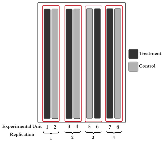
Figure 1.
An example of a randomized compete block design (RCBD) to evaluate if a treatment impacted outcomes, such as yield. In this example there is one control and one treatment strip per block (replication), and the trial is replicated four times. When farm equipment permits, strips serve as experimental units (EUs), which typically cover the length of a field [10].
The RCBD with field strips as EUs, however, poses challenges for both farmers and scientists. For farmers, it requires planning, and when yield from individual strips needs to be collected, it often slows down farm operations during planting and harvest, the busiest and most labor-intensive time of the year, effectively discouraging farmers to conduct OFE [11,12]. The design and its analysis pose challenges for scientists as well, because fields may only allow for three to four blocks to be implemented, which results in limited statistical power if each strip is one EU [7].
The arrival and more widespread adoption of yield monitoring systems now allow for yield data collection at a much higher spatial resolution (collection of data within strips). This enables documentation of spatial variability caused by a variety of different reasons, including non-uniform distribution of soil properties, soil moisture, pest pressure, rooting depth, and other factors [13]. For example, recent studies of corn (Zea mays L.) fields in New York have shown large variability in yield within fields [14,15]. The existence of such variability is well-recognized by both farmers and scientists [16]. However, until the arrival of reliable yield monitoring systems, the only way to deal with such variability in OFE was to conduct small plot research, where heterogeneity within fields is assumed to be small [9,17], or on a carefully chosen field with the least amount of spatial variability, based on farmers’ past experiences [18]. Results from such trials cannot be extended to other fields unless they have the same underlying conditions as the trial field [18]. In addition, it is quite possible for spatial variability within a field, even when selecting smaller experimental units, to mask any treatment effects being tested in OFE [19,20].
A single-strip treatment trial, also known as a demonstration plot by many, where a field is split into two (treatment versus control), is considerably easier to implement for farmers than a replicated trial with multiple strips in a field [21,22,23,24]. A single-strip treatment trial results in one response value (such as yield) for the treatment and the control. Response values are often derived by averaging multiple data points [7,21]. However, traditional statistical analyses such as ANOVA cannot be performed on a single-strip treatment trial as it only provides two to three EUs without replication. The validity of any inferences based on single-strip treatment trial is highly debated. While many [6,7,25,26] argue that concepts such as randomization, replications, and blocking should not be ignored for appropriate statistical analysis, some [1,24,27] argue that given the limited resources of farmers, single-strip treatment trials still provide useful information for decision making.
Given the ease of implementation of single strip EUs, a couple of studies have compared different statistical models for analyzing single strip evaluations, while taking into account the intensity of yield data collected with a yield monitor system (many data points per strip rather than just one value for the entire strip). Rudolph et al. [12] compared wheat (Triticum aestivum L.) yields in England using three strips varying in nitrogen (N) application (low, standard, and high). The entire field received a standard amount of N, while two strips received either 60 kg N ha−1 more (high) or 60 kg N ha−1 less (low) than the standard amount. The study compared outputs from statistical frameworks with and without taking into account spatial correlation, concluding that standard errors on the treatment effects were underestimated when spatial correlation is not considered. Lawes and Bramley [28] worked with farmers in Australia to analyze the effect of more versus less fertilizer for canola (Brassicus napus L.) and barley (Hordeum vulgare L.). For two fields, two management zones (low yielding vs. high yielding) were arbitrarily classified, based on the farmer’s intuition and past experience related to the field. For the third field, three management zones were delineated based on relative yield and electrical conductivity. In this study, ANOVA and ANOVA with spatial covariance, i.e., spatial ANOVA, were compared for quantifying the effect of fertilizer per zone. Contrary to Rudolph et al. [12], Lawes and Bramley [28] concluded that complex spatial analysis was not needed, as their approach produced similar results to the traditional statistical analysis.
While Lawes and Bramley [28] accounted for spatial variability of yield within each field using zones, they did not account for temporal yield variability, an important factor for understanding results of on-farm experimentation [15]. Temporal yield variability—heterogeneity in yield across multiple years at the field-level—can be caused by a variety of factors, including weather, management, and topography [29,30,31,32]. With availability of yield data from past years, both spatial and temporal yield variability over time can be assessed [14,15]. The main challenge remains whether we can design a statistically sound approach to treatment evaluation on farms, by farmers, given access to high resolution yield data, as well as to quantify both spatial and temporal yield variability.
Here we propose a statistical framework for estimating the treatment effect and standard error of the treatment effect (treatment versus control), based on yield monitor data from a single strip on-farm research trial, taking into account both spatial and temporal variability in yield to identify treatment signals, i.e., to reduce variability. It is important to note that we are differentiating the estimation of treatment effects and estimation of standard errors. For estimation of treatment effects, we explore two frameworks, namely least squares (LS) and generalized least squares with spatial covariance (GLS), while for estimation of standard errors, we explore two frameworks, that of assuming independence (Independence) and assuming spatial covariance (Spatial).
2. Materials and Methods
2.1. Yield Monitor Datasets
One dairy farm and one cash grain operation in central New York, USA, participated in this study. Single-strip N treatment trials were conducted in three site-years, two sites in 2018 and one site in 2019, per farm (Table 1). Corn was harvested for grain on the cash grain operation and for silage on the dairy farm. Yield monitor data on the six site-years, as well as the historic yield records of the farms (seven years of corn silage yield records for the dairy farm and five years of corn grain yield records for the cash grain operation), were used in the analysis. All yield data were collected using John Deere 3 (John Deere, Moline, IL, USA) systems. Raw yield monitor data were cleaned to eliminate systematic and random errors [33,34,35]. Pass overlap (driving over areas already harvested), incorrect yield estimates due to harvesting equipment slowing down or speeding up, and inconsistencies between sensor delays (flow and moisture delays) are examples of issues that contribute to errors in the raw yield monitor data [34]. Data were transformed in AgLeader format and exported in .CSV format using SMS Advanced Software (Ag Leader Technology, Ames, IA, USA). Yield Editor [36,37] was used for post-harvest data cleaning, as described in Kharel et al. [38] and based on Kharel et al. [34]. The yield cleaning protocol was used for all seven years of silage data and five years for grain data.

Table 1.
Crop type, year, field size, average yield production, number of data points from the yield monitor system, information about nitrogen strips, soil types, and distribution of management zones, delineated as suggested by Kharel et al. [15] for three fields on a grain operation (harvested for corn grain) and three on a dairy farm (harvested for corn silage).
2.2. Zone Delineation
Yield stability-based management zones, described in Kharel et al. [15], were delineated for each field with data through the year prior to strip implementation. Cleaned historic yield monitor data were interpolated using kriging with the Matérn covariance function with 2 × 2 m resolution [14]. Temporal average yield and standard deviation of yield were determined at the farm-level for farm-specific zone delineation [15]. The multi-year maps were compared against the farm-level average yield and the standard deviation to classify yield pixels (2 × 2 m) as high-yielding or low-yielding (above or below the farm average) and stable or unstable (below or above the farm-level temporal standard deviation). Pixels in Zones 1 and 4 represented stable yielding areas with high or low yields, respectively. Yields in Zones 2 and 3 were variable over time with, on average, yield above the farm average in Zone 2 and below average in Zone 3 (Table 1). Along with yield at the trial year, geolocation (provided by the yield monitor data) and the N application data points were assigned a zone based on yield of the past three or more years.
2.3. Single Strip Trial Design
For each site-year, a field-length single strip was placed where extra N was applied at or before planting. The placement of the single strip was chosen to intersect with a minimum of two management zones per field. The width of the strip was 9 m for the fields at the cash grain operation (Fields A, B, and C) and 24 m for the fields at the dairy farm (Field D, E, and F). At the grain operation, extra N was applied at a rate of 56 kg ha−1 as urea ammonium nitrate (UAN). At the dairy farm, the application rate was 121 kg ha−1, broadcasted as urea (Table 1). Two field-length strips located 10 m on the left and the right side of the N strip were identified as control strips for statistical analyses (Figure 2). Strips were at least two harvester widths wide (9 m for Field A, B, and C; 24 m for Field D, E, and F). With the exception of the N strips, which received higher N application rates at planting, fields were managed uniformly by the farmers, following land grant university guidance.
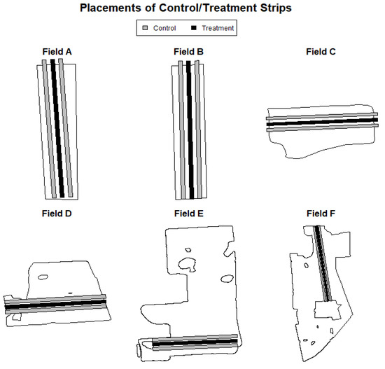
Figure 2.
Placements of nitrogen treatment strips (black) and control strips (grey) for three fields on a cash grain operation (Fields A, B, C) harvested for corn grain and three fields on a dairy farm harvested for silage (Fields D, E, F).
2.4. Statistical Modelling
Two approaches were explored for estimating the treatment effects: the least squares estimation, and the generalized least squares estimation with spatial covariance. The least squares estimation, , and the generalized least squares estimation, , of the treatment effects can be solved using the following formula:
where X is the design matrix containing data of the independent variables, y is a vector of the response, and Σ is the covariance matrix modeling the spatial dependence structure among data points. Isotropy, uniformity of variances in all directions, was assumed, and the Matérn covariance function was used to model spatial covariance [14]. The Matérn covariance function is parametrized as:
where covariance parameters are variance, range, smoothness, and nugget, for two GNSS co-ordinates and . The nugget value is added to the diagonal of the covariance matrix. is a gamma function, and is the modified Bessel function of the second kind [14]. The parameters for the covariance function were estimated through maximum likelihood estimation using the GpGp package [39]:
Both and and are P × N matrices, where P is the number of explanatory variables, and N is the number of data points. Multiplying or by the response vector, y, results in a vector of the beta coefficients with M elements. Standard errors, the level of uncertainties around treatment effects estimation, can be calculated by using the following general formula:
where M is either or , depending on the treatment estimation approach, and K is a covariance matrix. Two approaches were explored for estimating the standard errors, namely assuming independence and assuming spatial covariance. If we assume independence, the covariance matrix K would be , where where is the response, is the model prediction, N is the number of data points, and I is the identity matrix. If we take into account spatial covariance, K, would be Σ, as described above.
The estimation of treatment effects and standard errors often is treated as a single problem instead of two independent ones. In statistics, least squares estimation refers to the estimation of treatment effect via (1) and estimation of standard errors assuming independence, which is . In this study, however, we treated estimation of treatment effects and standard errors as two separate problems to closely analyze each approach. Treating treatment effects and standard errors as two separate problems is not uncommon in the field of spatial statistics, as suggested by Cressie and Wikle [40], mainly due to the heavy computational cost associated with estimating parameters for the spatial covariance function. We argue that it also provides a more appropriate framework to analyze single strip treatment trials.
Four possible combinations of the treatment effects and standard errors estimations exist: (a) the least squares estimation, with independence assumption for standard errors; (b) the least squares estimation, with spatial covariance for standard errors; (c) the generalized least squares estimation, with independence assumption for standard errors; and (d) the generalized least squares estimation, with spatial covariance for standard errors. Approach (a) is referred to as LS 1, (b) is referred to as LS 2, and (d) is referred to as GLS from here on. Of the four approaches, (c) was excluded from the analysis because it was deemed inferior to the other approaches, as explained in Results, Model Diagnostics.
2.5. Explanatory Variables Selection and Model Fitting
It is reasonable to believe, as these fields were managed uniformly by the same farm over the past years, that yield data measured with a yield monitor system are both spatially and temporally correlated, i.e., yield estimates that are located closer together tend to have similar values when compared to points that are further apart. A location that is historically high yielding over the past years and has consistently been that way, thus, is likely to exhibit high yield in the following years.
Exploratory data analysis on the spatial and temporal yield distribution within the field was performed to appropriately control for such spatial autocorrelation when estimating the effect of N treatment.
To account for intra-field spatial yield variation, relative latitude and longitude and their linear interaction were treated as fixed effects. Relative latitude and longitude were calculated by subtracting the average value of each, i.e., the goal was to anonymize the location of the field. We could possibly control for linear yield trend across the field, due to topographic factors within the field, by adding these factors as fixed effects. Spatial yield variation also was considered under the statistical modeling. LS 2 considers the spatial covariance structure, Σ, when estimating standard errors, while GLS uses it when estimating both treatment effects and standard errors estimation. On the other hand, LS 1 assumes that each data point is independent when estimating both the treatment effects and the standard errors.
Temporal yield variability, or heterogeneity in yield across multiple years, also needed to be accounted for to accurately examine the effect of the treatment and its standard error. Temporal average yield, estimated by averaging over the past years at the given location, was treated as a fixed effect to control for the historic yield level of the field. In addition, management zones, as described in Kharel et al. [15], and its interactions with N treatment were treated as fixed effects to control for temporal yield level and its variation at the farm level. The interaction term between four management zones and N treatment was added because yield response to N was expected to differ among management zones. Thus, the following model was fitted via three approaches, as mentioned above (LS 1, LS 2, and GLS), using the R base package [41] and GpGp [39]:
where Yield is the response variable representing the yield at the site-year during the trial, Zone is the management zone (Zone 1, 2, 3, or 4), Nitrogen is the binary variable representing whether the data point was either located in the N strip (Nitrogen = 1) or one of the two control strips (Nitrogen = 0), AverageYield is the temporal average yield, calculated based on the past yield data at the given location, and Latitude and Longitude are the normalized geolocation of the data points. A design matrix, X, and the response vector, y, were formed based on Formula (6) and were used to estimate the treatment effects and their standard errors (see Statistical Modelling under Materials and Methods). Treatment effects and standard errors—estimated per LS 1, LS 2, and GLS—were first compared.
2.6. Model Output and Diagnostics
As noted, treatment effects for extra N per management zone were estimated using two approaches: the LS approach (1), and the GLS approach (2). The treatment effects in both cases can be represented via a linear combination of the responses. This means that the treatment effects, either or , can be viewed as a weighted sum of the response vector y. Under this framework, , (3), for the LS approach and , (4), for the GLS approach can be thought of as the aforementioned weights. In other words, for some entry, j, of treatment effects vector, :
where is the amount of weight assigned to a response among n data points within a field. Distributions of for the LS and the GLS approaches were analyzed to identify the better approach for estimating the treatment effects of extra nitrogen per zone.
The stability of estimates using the LS approach (LS 1 and LS 2) and the GLS approach also were measured. Given a sufficient number of data points to start with, the number of data points should not significantly affect the estimated treatment effects. Additionally, yield monitor data point can be missing, removed during the data-cleaning process, or otherwise not recorded. Thus, the approach that provides stable estimates with respect to missing values was deemed more appropriate. Difference in estimates, when a portion of the data were used versus when all the data points were used, was compared to measure stability of the estimate. The treatment effects estimated using the randomly selected 60% of the data for a site year, using the two approaches (LS and GLS), were compared against the treatment effects estimated using 100% of the data. The root mean squared error (RMSE) was calculated by repeating this process 100 times:
where represents the estimate using 60% of the data, indexed between i = 1 and 100, and represents the estimate using 100% of the data. The approach with the smaller RMSE was deemed more stable and therefore more appropriate when estimating the treatment effects for a single-strip treatment trial.
3. Results
3.1. Yield in Control and Nitrogen Strips
For the grain fields, the average yield in the N treatment strip was 0.22 and 0.26 Mg ha−1 (85% DM) higher for Field B and C, respectively, while for Field A it was 0.12 Mg ha−1 lower. For the silage fields, the treatment strip was higher yielding on average for field D and E (2.38 and 5.20 Mg ha−1 higher at 35% DM, respectively), while for Field F, the control strips yielded higher than the treatment strips by 2.32 Mg ha−1 (Figure 3). The overall yield distributions were similar across fields, with a standard deviation between 0.5 and 1.0 Mg ha−1 for grain fields (Field A, B, and C) and between 10 and 13 Mg ha−1 for the silage fields (Field D, E, and F).
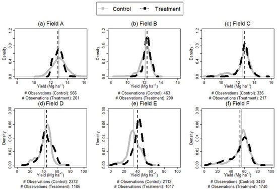
Figure 3.
Density plot representing corn yield distributions of a N treatment strip (higher N) and the neighboring control strips. The dotted black and the solid grey vertical lines represent the average yield for the N treatment strip and the control strips, respectively. Fields A, B, C (a–c) were harvested for grain. Fields D, E, F (d–f) were harvested for silage.
The differences in yield between the N strips and their controls varied greatly among zones (Figure 4). For example, while on average the control strips were higher yielding than the N treatment for Field A, analysis per zone showed a positive response of 0.25 Mg ha−1 for Zone 2, while in Zone 1, yield in the N strip was 0.25 Mg ha−1 lower than in the control. Similarly, for Field C, the yield in the N strip was higher across the field, primarily because of a large yield increase in Zone 3 (1.66 Mg ha−1), while average yield in Zone 1 was 0.11 Mg ha−1 lower than in the control. For Fields B, D, E, and F, the difference in average yield between treatment and control per zone was consistent with differences measured at the field-level. For Field B, D, and E, where the treatment strips were higher-yielding than the control strips on average, the yield from treatment strips were higher-yielding than the control strips per zone as well. Field F exhibited lower yield in the N strip, consistent for all zones in the field. The conclusion as to whether these differences are statistically significant were analyzed through various statistical frameworks in the following sections.
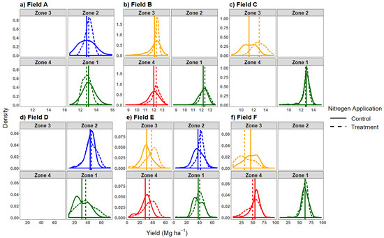
Figure 4.
Density plots representing corn yield distribution of N treatment and control strips in individual fields, with up to four yield stability zones, as per Kharel et al. [15]. The dotted and the solid vertical line represent the average yield for the treatment and control strip, respectively. Fields A, B, C (a–c) were harvested for grain. Fields D, E, F (d–f) were harvested for silage.
3.2. Spatio-Temporal Yield Variation
Yield, as well as the spatial distribution of yield, varied greatly within each field (Figure 5). The standard deviation of yield, a measure of spatial yield variation, was between 0.5 and 0.8 Mg ha−1 for the grain fields (Fields A, B, and C) and 8 and 12 Mg ha−1 for the silage fields (Fields D, E, and F). Linear relationships between spatial coordinates and yield were present in Field A. Data points on the west side of the field tended to be higher-yielding than the data points on the eastside of the field (Figure 5a). Because of a risk of such within-field trends, spatial coordinates and their linear interaction were added as fixed effects in the overall statistical model.
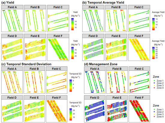
Figure 5.
Spatial distribution of yield (a), historic average yield (b), temporal standard deviation (c), and management zones (d), as estimated based on previous years of yield produced for six fields (A through F). Yield stability management zones were delineated as described in Kharel et al. [15]. Zone 1 represents high-yielding-stable, Zone 2 represents high-yielding–unstable, Zone 3 represents low-yielding–unstable, and Zone 4 represents low-yielding–stable areas of the field.
Overall, yield estimates that were in closer proximity tended to have similar values (Figure 5a). Some data points, however, exhibited distinctly different yield estimates when compared against nearing data points. Such data points were often, but not always, located at intersections of main areas in a field and headland areas where compaction, pest pressure, and shading could impact yield [42]. Spatial autocorrelation of yield estimates was also evident from the semi-variograms (Figure 6). All six fields, especially Field C, E, and F, exhibited spatial autocorrelation consistent with the Matérn covariance function. At large spatial lags, all six fields showed unusual values. This was due to the low number of data points separated by large distances, and thus the variogram estimator was known to be inaccurate at large distances.
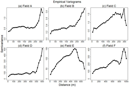
Figure 6.
An empirical variogram for corn yield for six fields (Fields A–F) based on the yield estimates from the yield monitor and their corresponding spatial coordinates. Fields A, B, C (a–c) were harvested for grain. Fields D, E, F (d–f) were harvested for silage.
The spatial distribution of temporal average yields, calculated using the yield data prior to the trial, showed a similar yield distribution when compared against the spatial distribution of yield during the trial year (Figure 5a,b). For example, the middle strip in Field C yielded higher than the rest of the field, both historically (Figure 5b) and in the trial year. It is important to note that the middle strip was the location where the extra nitrogen was applied during the trial year. Temporal average yield was included as fixed effect in the overall statistical model, to control for the historic level of production at the field-level.
Within the same farm, the temporal average yield differed by field (Figure 5b). For corn grain, Fields A and C were high-yielding, while Field B had a wide range in yield within the field. For corn silage, Field D was high-yielding, Field E had yields similar to the average yield production of the farm, and Field F was lower-yielding. Yield temporal variation was also noticeably different, especially for grain fields (Figure 5c). For all three silage fields, temporal yield variation was generally low across the field. For grain fields, Field D had high temporal yield variation, while Field F had low yield variation. The temporal average yield and its variation at the farm-level were captured by the four yield stability-based management zones, as described by Kharel et al. [15] (Figure 5d). Such management zones can be used to account for both the average level of production and its variation across time at the farm-level. Thus, management zones, as well as their interaction with N treatment, were added as fixed effects in the overall statistical model.
3.3. Model Outputs
Treatment effects per zone for each field were noticeably different, depending on the method used for the estimation (LS 1 and 2 vs. GLS; Table 2). For example, the N effect for Zone 1 for Field A via LS was −0.23 Mg ha−1, implying that addition of N decreased yield by 0.23 Mg ha−1 for Zone 1. However, it was 0.45 Mg ha−1 when the GLS approach was used, suggesting a higher yield for the N strip. The treatment effects of LS 1 and LS 2 were both estimated using the least squares approach, thus resulting in the same outputs. Standard errors estimated assuming independence (LS) and spatial correlation (LS 2 and GLS) also showed noticeable difference. For all fields, standard errors assuming spatial covariance (LS 2 and GLS) were greater, providing a more conservative estimation when compared to those estimated assuming independence (LS). Such differences were likely due to spatial autocorrelation, as evident in Figure 5 and Figure 6. The differences in standard error between LS 2 and GLS also were noticeable. For all cases, GLS led to smaller estimations of standard error than LS 2, and such difference was due to the property of the GLS estimator. The GLS estimator of treatment effects (4) was proven to have the smallest error variance among all possible linear combinations of the data, including LS (1) [43].
Table 2.
A regression model with the yield as the response variable, temporal average yield, latitude, longitude, linear interaction between latitude and longitude, and four corn management zones, delineated as suggested by Kharel et al. [15], and their interaction with N treatment as the explanatory variables (see Equation (7) for the model details) were summarized for six fields (Fields A, B, C, D, E, and F). Each nitrogen effect per management zone was estimated. For LS 1, least squares was used for treatment effects, and independence was assumed for standard errors. For LS 2, least squares was used for treatment effects, and spatial covariance was used for standard errors. For GLS, generalized least squares was used for treatment effects, and spatial covariance was used for standard errors. Fields A, B, and C were harvested for grain. Fields D, E, and F were harvested for silage.
3.4. Model Diagnostics
The coefficients for the LS approach, showed relatively uniform values across the field, when compared to coefficients for the GLS approach, (Figure 7). The coefficient for the GLS approach presented unusual outliers across the fields. These outliers were attributed to sharp changes between explanatory variables that were in close proximity. Unlike the LS approach, which puts equal weight across data points due to the independence assumption, GLS puts more weight on two data points that are in close proximity but have a drastic difference in their explanatory variables (i.e., management zones). As we observed in Figure 5, there are many data points that are close in distance but occupy different management zones.
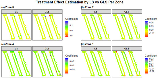
Figure 7.
Spatial distribution of coefficients for estimating treatment effect of N treatment per yield stability-based management zone (Zone 1, 2, 3, and 4) via the least squares method (LS) and generalized least squares (GLS) method for Field A. Coefficients for LS were calculated by solving and for GLS by solving , where X represents the design matrix and Σ the spatial covariance.
The challenge of estimating the treatment effect with a categorical explanatory variable, while also accounting for spatial covariance structure, was noted by Griffin et al. [21]. The authors called it the “neighboring observation problem” and pointed out that observations that are located on the edge of different treatments influence the power of estimating the treatment differences. To bypass this problem, the LS approach was proposed for estimating the treatment effects per management zone.
The LS approaches (LS 1 and LS 2) also were shown to be more stable than the GLS approach for estimating the treatment effects (Table 3). For all six fields and four management zones, the RMSEs, comparing estimates using 60% and 100% of the data, were smaller for the LS approach than those of the GLS approach. This observation also is corroborated by the comparison between and in Figure 7. Based on these observations, the LS estimation for the treatment effect is more appropriate when compared against the GLS estimation, as LS is more robust in its estimation, regardless of the number of observations.
Table 3.
Root mean squared errors (RMSEs) were calculated per management zones (Zone 1, 2, 3, and 4) and field (Field A, B, C, D, E, and F) comparing treatment effect estimates using 60% and 100% of the data. Two approaches, least squares (LS) and generalized least squares (GLS) approaches, were used to estimate the treatment effects.
4. Discussion
In this work, we proposed an alternative statistical framework to analyze a non-replicated single strip treatment trial. By leveraging high resolution spatial yield monitor data as well as temporal variability in yield, we aim to make OFE more feasible for farmers while gaining as much insight as possible from un-replicated strips. We differentiated the estimation of treatment effects and estimation of standard errors. For estimation of treatment effects, we explored two frameworks, namely least squares (LS) and generalized least squares with spatial covariance (GLS), while for estimation of standard errors, we explored two frameworks, that of assuming independence (Independence) and assuming spatial covariance (Spatial). Our conclusion was that LS is more appropriate in estimating the treatment effect while Spatial provides more reasonable estimation of standard error than Independence.
Literature such as Rudolph et al. [12] also compared outputs from statistical frameworks with and without taking into account spatial autocorrelation and concluded that standard errors of the treatment effects were underestimated when spatial correlation was not considered; our results corroborated this finding. For all six fields, standard errors estimated with spatial covariance were distinctively larger than standard errors estimated assuming independence. This finding also corroborates many studies that evaluated the importance of spatial yield variability at the field level [14,15,21,33]. However, our results contradicted those by Lawes and Bramley [28], who concluded that a comparison between data points, without taking into account spatial covariance, and linear model estimation with spatial covariance, did not produce significantly different results. Our analysis suggests that the effects of N are drastically different when the LS approach, a model that assumed independence, or the GLS approach, a model that considers spatial covariance, are used. The noticeable difference between our analysis and that of Lawes and Bramley [28] may be attributed to the use of yield stability-based management zones in our study. We analyzed the impact of N per yield stability-based management zones, delineated according to Kharel et al. [15], which provides information about both the temporal average yield and its variation in relation to the farm-level temporal average yield and its variation. While Lawes and Bramley [28] used management zones, they did not take into account spatial yield trends nor yield variability caused by a variety of factors, including the weather, management, and topography [29,30,31,32]. Temporal and spatial yield variation within a field can be high in New York, and it is crucial to take into account this variability to appropriately estimate the effect of a treatment from an OFE.
We acknowledge that historic yield record or other data channels are not always available for researchers and farmers to generate management zones. In such case, concepts such as randomization, replications, and blocking should be implemented to accurately estimate the treatment effect, as suggested by [6,7,25,26], to prevent biased estimation of treatment effects. Additionally, our analysis assumed isotropy, uniformity of variances in all directions, and uniform spatial correlation across all three strips. While Matérn isotropic covariance was able to account for spatial variability in yield shown in the data, one may want to implement a non-stationary spatial model as shown in Jin et al. [44], for example, to account for potentially more complicated spatial covariance structures. Jin et al. [44] proposed the use of sampling-based localized co-kriging developed in Cressie and Wikle [40].
5. Conclusions
It remains obvious, from a practical perspective, that for farmers interested in on-farm evaluation of a change in management, a single strip field evaluation is much easier to implement than multi-strip trials. We thus explored approaches for estimating the effect of the treatment and uncertainty around that estimation (standard error) for a single strip treatment trial. The results of this study show that when yield is documented using yield monitor systems that collect georeferenced yield data per second, variability within a field can be quantified per management zones. With high resolution zone maps and spatial covariance, treatment effects from a single-strip treatment trial effectively can be estimated. We therefore propose the use of LS 2, i.e., estimation of treatment effects using the LS approach and standard errors with spatial covariance, for analyzing responses, such as yield or other desired outcomes, from a specific management change or treatment. Through this approach, we can estimate the effect of a treatment and standard errors from any un-replicated, single-strip OFE, based on historic yield monitor data and yield stability-based management zones. Moreover, it allows for more field trial data to be added over time for better understanding of drivers for outcomes such as yield and the need for site-specific management in unstable yielding zones.
Author Contributions
Conceptualization, Q.M.K., J.B.C. and J.G.; methodology, J.B.C., J.G., T.K. and Q.M.K.; validation, J.B.C., J.G.; formal analysis, J.B.C. and J.G.; investigation, J.B.C., Q.M.K., T.K., and J.G.; resources, Q.M.K.; data curation, Q.M.K., T.K., and Á.M.; writing—original draft preparation, J.B.C.; writing—review and editing, J.B.C., J.v.A., Q.M.K., T.K., Á.M. and J.G.; visualization, J.B.C., Q.M.K., and J.G.; supervision, J.v.A., Q.M.K. and J.G.; project administration, Q.M.K. and J.G.; funding acquisition, Q.M.K. and K.J.C. All authors have read and agreed to the published version of the manuscript.
Funding
This research was funded with grants from the New York Farm Viability Institute, the United States Department of Agriculture, National Institute of Food and Agriculture, Agriculture and Food Research Initiative (USDA-NIFA-AFRI-004915) Bioenergy, Natural Resources and Environment (BNRE) program, Federal Formula Funds, and grants from the Northern New York Agricultural Development Program (NNYADP) and New York Corn Growers Association (NYCGA) Any opinions, findings, conclusions, or recommendations expressed in this publication are those of the author(s) and do not necessarily reflect the view of the USDA or other funding sources.
Institutional Review Board Statement
No applicable.
Informed Consent Statement
No applicable.
Data Availability Statement
No applicable.
Conflicts of Interest
The authors declare no conflict of interest.
References
- Mutsaers, H.J.W.; Agriculture, I.I.O.T. A Field Guide for On-Farm Experimentation; International Institute of Tropical Agriculture: Ibadan, Nigeria, 1997. [Google Scholar]
- Petersen, R.G. Agricultural Field Experiments: Design and Analysis; Taylor & Francis: London, UK, 1994. [Google Scholar]
- Kyveryga, P.M. On-Farm Research: Experimental Approaches, Analytical Frameworks, Case Studies, and Impact. Agron. J. 2019, 111, 2633–2635. [Google Scholar] [CrossRef] [Green Version]
- Federer, W.T. Experimental Design: Theory and Application; Macmillan: New York, NY, USA, 1955. [Google Scholar]
- Little, T.M.; Hills, F.J. Agricultural Experimentation: Design and Analysis; Wiley: Hoboken, NJ, USA, 1978. [Google Scholar]
- Kyveryga, P.M.; Mueller, T.A.; Mueller, D.S. On-Farm Replicated Strip Trials. In Precision Agriculture Basics; American Society of Agronomy: Madison, WI, USA, 2018; pp. 189–207. [Google Scholar]
- Piepho, H.-P.; Richter, C.; Spilke, J.; Hartung, K.; Kunick, A.; Thöle, H. Statistical aspects of on-farm experimentation. Crop Pasture Sci. 2011, 62, 721–735. [Google Scholar] [CrossRef]
- Gotway Crawford, C.A.; Bullock, D.G.; Pierce, F.J.; Stroup, W.W.; Hergert, G.W.; Eskridge, K.M. Experimental Design Issues and Statistical Evaluation Techniques for Site-Specific Management. In The State of Site Specific Management for Agriculture; American Society of Agronomy: Madison, WI, USA, 1997; pp. 301–335. [Google Scholar]
- Fisher, R.A. The Arrangement of Field Experiments. J. Minist. Agric. 1926, 33, 503–515. [Google Scholar] [CrossRef]
- Kyveryga, P.; Mueller, T.; Paul, N.; Arp, A.; Reeg, P. Guide to On-Farm Replicated Strip Trials; Iowa Soybean Association: Ankeny, IA, USA, 2015. [Google Scholar]
- Griffin, T.W.; Lambert, D.M.; Lowenberg-DeBoer, J.M. Testing Appropriate On-Farm Trial Designs and Statistical Methods for Precision Farming: A Simulation Approach; Precision Agriculture Center, University of Minnesota, Department of Soil, Water and Climate: St. Paul, MN, USA, 2004; pp. 1733–1748. [Google Scholar]
- Rudolph, S.; Marchant, P.; Gillingham, V.; Kindred, D.; Sylvester-Bradley, R. Spatial Discontinuity Analysis’a novel geostatistical algorithm for on-farm experimentation. In Proceedings of the 13th International Conference on Precision Agriculture, St. Louis, MO, USA, 31 July–3 August 2016. [Google Scholar]
- Sawyer, J.E. Concepts of Variable Rate Technology with Considerations for Fertilizer Application. J. Prod. Agric. 1994, 7, 195–201. [Google Scholar] [CrossRef]
- Cho, J.B.; Guinness, J.; Kharel, T.P.; Sunoj, S.; Kharel, D.; Oware, E.K.; van Aardt, J.; Ketterings, Q.M. Spatial estimation methods for mapping corn silage and grain yield monitor data. Precis. Agric. 2021, 22, 1501–1520. [Google Scholar] [CrossRef]
- Kharel, T.P.; Maresma, A.; Czymmek, K.J.; Oware, E.K.; Ketterings, Q.M. Combining Spatial and Temporal Corn Silage Yield Variability for Management Zone Development. Agron. J. 2019, 111, 2703–2711. [Google Scholar] [CrossRef]
- Fisher, R.A. Principles of Plot Experimentation in relation to the Statistical Interpretation of the Results. In Proceedings of the Rothamsted Conferences, 13: The Technique of Field Experiments, Harpenden, UK, 7 May 1931; under the Chairmanship of Sir A. D. Hall. Rothamsted Experimental Station: Harpenden, UK, 1931; pp. 11–13. [Google Scholar]
- Oehlert, G.W. A First Course in Design and Analysis of Experiments; W. H. Freeman: New York, NY, USA, 2000. [Google Scholar]
- Gomez, K.A.; Gomez, A.A. Statistical Procedures for Agricultural Research; Wiley: Hoboken, NJ, USA, 1984. [Google Scholar]
- Kim, S.; Daughtry, C.; Russ, A.; Pedrera-Parrilla, A.; Pachepsky, Y. Analysis of Spatiotemporal Variability of Corn Yields Using Empirical Orthogonal Functions. Water 2020, 12, 3339. [Google Scholar] [CrossRef]
- Panten, K.; Bramley, R.G.V.; Lark, R.M.; Bishop, T.F.A. Enhancing the value of field experimentation through whole-of-block designs. Precis. Agric. 2010, 11, 198–213. [Google Scholar] [CrossRef]
- Griffin, T.W.; Florax, R.J.G.M.; Lowenberg-DeBoer, J. Field-Scale Experimental Designs and Spatial Econometric Methods for Precision Farming: Strip-Trial Designs for Rice Production Decision Making. In Proceedings of the 2006 Annual Meeting, Orlando, FL, USA, 5–8 April 2006. [Google Scholar]
- Lambert, D.M.; Lowenberg-Deboer, J.; Bongiovanni, R. A Comparison of Four Spatial Regression Models for Yield Monitor Data: A Case Study from Argentina. Precis. Agric. 2004, 5, 579–600. [Google Scholar] [CrossRef]
- Willers, J.L.; Milliken, G.A.; Jenkins, J.N.; O’Hara, C.G.; Gerard, P.D.; Reynolds, D.B.; Boykin, D.L.; Good, P.V.; Hood, K.B. Defining the experimental unit for the design and analysis of site-specific experiments in commercial cotton fields. Agric. Syst. 2008, 96, 237–249. [Google Scholar] [CrossRef]
- Yan, W.; Hunt, L.A.; Johnson, P.; Stewart, G.; Lu, X. On-Farm Strip Trials vs. Replicated Performance Trials for Cultivar Evaluation. Crop Sci. 2002, 42, 385–392. [Google Scholar] [CrossRef] [Green Version]
- Cox, D.R. Randomization in the Design of Experiments. Int. Stat. Rev. 2009, 77, 415–429. [Google Scholar] [CrossRef]
- Johnson, D.H. The Many Faces of Replication. Crop Sci. 2006, 46, 2486–2491. [Google Scholar] [CrossRef]
- Stroup, W.W.; Hildebrand, P.E.; Francis, C.A. Farmer Participation for More Effective Research in Sustainable Agriculture. In Technologies for Sustainable Agriculture in the Tropics; American Society of Agronomy: Madison, WI, USA, 1993; pp. 153–186. [Google Scholar]
- Lawes, R.A.; Bramley, R.G.V. A Simple Method for the Analysis of On-Farm Strip Trials. Agron. J. 2012, 104, 371–377. [Google Scholar] [CrossRef]
- Andresen, J.A.; Alagarswamy, G.; Rotz, C.A.; Ritchie, J.T.; LeBaron, A.W. Weather Impacts on Maize, Soybean, and Alfalfa Production in the Great Lakes Region, 1895–1996. Agron. J. 2001, 93, 1059–1070. [Google Scholar] [CrossRef] [Green Version]
- Kravchenko, A.N.; Robertson, G.P.; Thelen, K.D.; Harwood, R.R. Management, Topographical, and Weather Effects on Spatial Variability of Crop Grain Yields. Agron. J. 2005, 97, 514–523. [Google Scholar] [CrossRef] [Green Version]
- Mallory, E.B.; Porter, G.A. Potato Yield Stability under Contrasting Soil Management Strategies. Agron. J. 2007, 99, 501–510. [Google Scholar] [CrossRef]
- Smith, R.G.; Menalled, F.D.; Robertson, G.P. Temporal Yield Variability under Conventional and Alternative Management Systems. Agron. J. 2007, 99, 1629–1634. [Google Scholar] [CrossRef] [Green Version]
- Dobermann, A.; Ping, J.L. Geostatistical Integration of Yield Monitor Data and Remote Sensing Improves Yield Maps. Agron. J. 2004, 96, 285–297. [Google Scholar] [CrossRef]
- Kharel, T.P.; Swink, S.N.; Maresma, A.; Youngerman, C.; Kharel, D.; Czymmek, K.J.; Ketterings, Q.M. Yield Monitor Data Cleaning is Essential for Accurate Corn Grain and Silage Yield Determination. Agron. J. 2019, 111, 509–516. [Google Scholar] [CrossRef]
- Vega, A.; Córdoba, M.; Castro-Franco, M.; Balzarini, M. Protocol for automating error removal from yield maps. Precis. Agric. 2019, 20, 1030–1044. [Google Scholar] [CrossRef]
- Sudduth, K.A.; Drummond, S.T. Yield Editor: Software for Removing Errors from Crop Yield Maps. Agron. J. 2007, 99, 1471–1482. [Google Scholar] [CrossRef]
- Sudduth, K.A.; Drummond, S.T.; Brenton Myers, D. Yield Editor 2.0: Software for Automated Removal of Yield Map Errors. In 2012 Dallas, Texas, July 29–August 1, 2012; American Society of Agricultural and Biological Engineers: St. Joseph, MI, USA, 2012. [Google Scholar]
- Kharel, T.P.; Swink, S.N.; Youngerman, C.; Maresma, A.; Czymmek, K.J.; Ketterings, Q.M.; Kyveryga, P.; Lory, J.; Musket, T.A.; Hubbard, V. Processing/Cleaning Corn Silage and Grain Yield Monitor Data for Standardized Yield Maps across Farms, Fields, and Years; Cornell University, Nutrient Management Spear Program, Department of Animal Science: Ithaca, NY, USA, 2018. [Google Scholar]
- Guinness, J.; Katzfuss, M. GpGp: Fast Gaussian Process Computation Using Vecchia’s Approximation. R package 0.3.2. 2019. Available online: https://CRAN.R-project.org/package=GpGp (accessed on 1 October 2021).
- Cressie, N.; Wikle, C.K. Statistics for Spatio-Temporal Data; Wiley: Hoboken, NJ, USA, 2011. [Google Scholar]
- R Core Team. R: A Language and Environment for Statistical Computing; R Foundation for Statistical Computing: Vienna, Austria, 2019. [Google Scholar]
- Sunoj, S.; Kharel, D.; Kharel, T.; Cho, J.; Czymmek, K.J.; Ketterings, Q.M. Impact of headland area on whole field and farm corn silage and grain yield. Agron. J. 2021, 113, 147–158. [Google Scholar] [CrossRef]
- White, T.L.; Hodge, G.R. Best Linear Unbiased Prediction: Applications. In Predicting Breeding Values with Applications in Forest Tree Improvement; Springer: Dordrecht, The Netherlands, 1989; pp. 300–327. [Google Scholar]
- Jin, H.; Shuvo Bakar, K.; Henderson, B.L.; Bramley, R.G.V.; Gobbett, D.L. An efficient geostatistical analysis tool for on-farm experiments targeted at localised treatment. Biosyst. Eng. 2021, 205, 121–136. [Google Scholar] [CrossRef]
Publisher’s Note: MDPI stays neutral with regard to jurisdictional claims in published maps and institutional affiliations. |
© 2021 by the authors. Licensee MDPI, Basel, Switzerland. This article is an open access article distributed under the terms and conditions of the Creative Commons Attribution (CC BY) license (https://creativecommons.org/licenses/by/4.0/).