Energy, Production and Environmental Characteristics of a Conventional Weaned Piglet Farm in North West Spain

 , ,
, ,  ,
, 
Abstract
1. Introduction
2. Materials and Methods
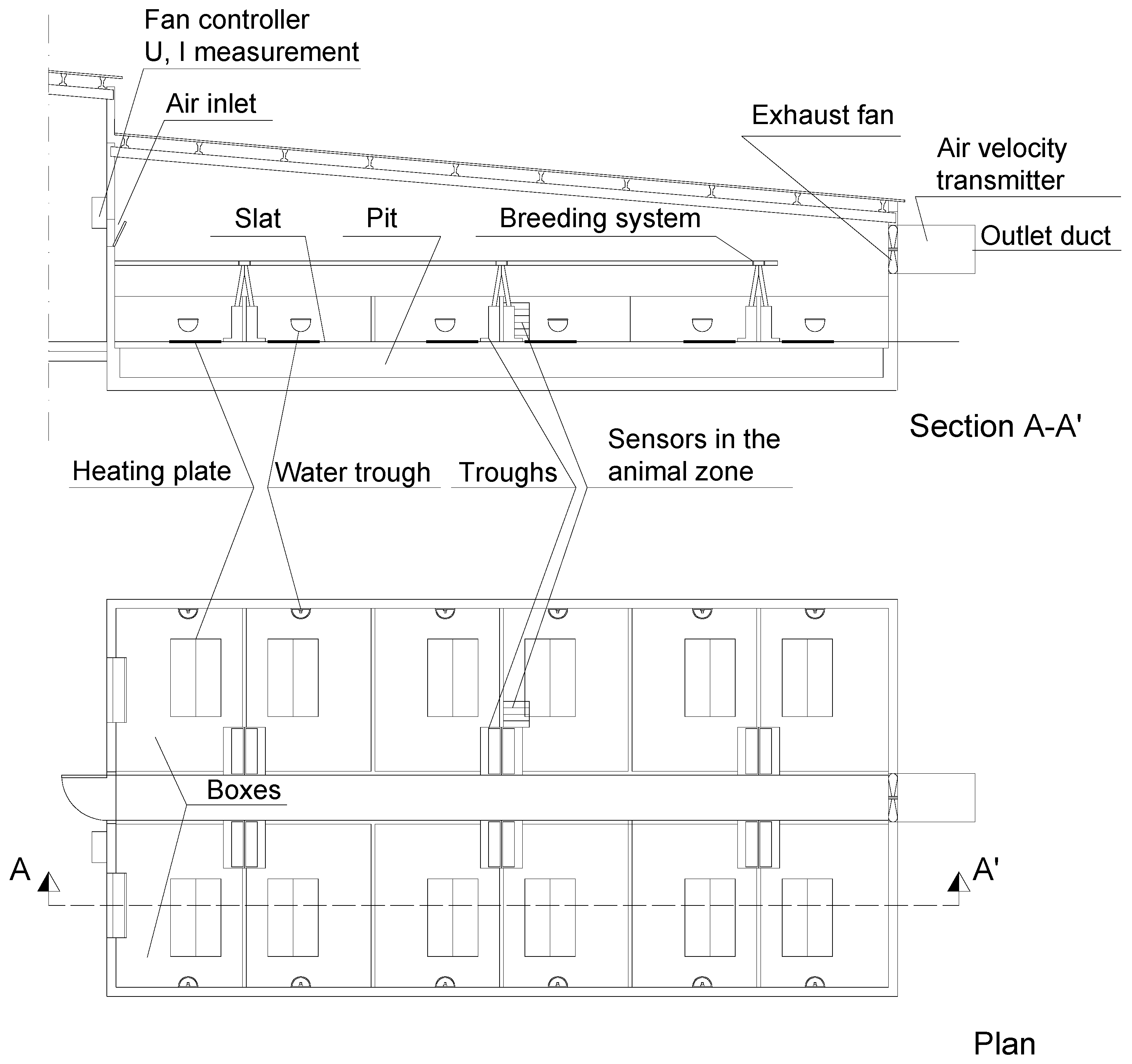
2.1. Measurement and Determination of Variables
- Humidity (HR) and temperature (T) in the animal zone were measured using S-THB-008 sensors (Onset Computer Corporation), with measurement ranges of 0% to 100% and −40 °C to 75 °C.
- CO2 concentration in the animal zone (CCO2) was measured using Delta Ohm HD37BTV.1 transmitters with double-wave infrared technology (NDIR) and a measurement range of 0–5000 ppm.
- Air velocity in the animal zone (v) was measured using a Delta Ohm HD103T.0 omnidirectional hotwire probe, with measurement range of 0.08–5 m s−1.
- Flow of the heating system (Qhs): Siemens SITRANS F US Clamp-on FST020 IP65 NEMA 4X ultrasonic flowmeter.
- Temperature at the inlet (Ti) and outlet (To) of the heating system: Campbell Scientific Ltd. model 108, with a measurement range of −5°–+95 °C, >±0.5 °C.
- Fan operating voltage (U): Magnelab AC Potential Transformer (PT) T-MAG-SPT-600 (Onset Computer Corporation), which, connected to an Onset Computer Corporation TRSM module, provided effective value.
- Fan operating current (I): Magnelab AC Current Transformer SCT-0750-050 (Onset Computer Corporation), which, connected to an Onset Computer Corporation TRSM module, provided effective value.
- Velocity of the air extracted through the ventilation system (vm): Delta Ohm HD2903TTC310 active air velocity transmitter installed at the fan outlet according to the method described by the authors of [31] and adapted to the hotwire probe.
2.2. Statistical Methods
3. Results
4. Discussion
Author Contributions
Funding
Conflicts of Interest
References
- Massari, J.M.; Moura, D.J.D.; Curi, T.M.D.C.; Vercellino, R.D.A.; Medeiros, B.B. Zoning of environmental conditions inside a wean-to-finish pig facility. Eng. Agríc. 2016, 36, 739–748. [Google Scholar] [CrossRef]
- Le Dividich, J.; Herpin, P. Effects of climatic conditions on the performance, metabolism and health-status of weaned piglets: A review. Livest. Prod. Sci. 1994, 38, 79–90. [Google Scholar] [CrossRef]
- Gilbert, H.; Ruesche, J.; Muller, N.; Billon, Y.; Begos, V.; Montagne, L. Responses to weaning in two pig lines divergently selected for residual feed intake depending on diet. J. Anim. Sci. 2019, 97, 43–54. [Google Scholar] [CrossRef] [PubMed]
- Lu, X.; Zhang, M.; Zhao, L.; Ge, K.; Wang, Z.; Jun, L.; Ren, F. Growth performance and post-weaning diarrhea in piglets fed a diet supplemented with probiotic complexes. J. Microbiol. Biotechnol. 2018, 28, 1791–1799. [Google Scholar] [CrossRef] [PubMed]
- Saha, C.K.; Zhang, G.; Kai, P.; Bjerg, B. Effects of a partial pit ventilation system on indoor air quality and ammonia emission from a fattening pig room. Biosyst. Eng. 2010, 105, 279–287. [Google Scholar] [CrossRef]
- Pedersen, S.; Jørgensen, H.; Theil, P.K. Influence of diurnal variation in animal activity and digestion on animal heat production. Agric. Eng. Int. CIGR J. 2015, 18–29, Special issue: 18th World Congress of CIGR. [Google Scholar]
- Dolz, N.; Babot, D.; Álvarez-Rodríguez, J.; Forcada, F. Improving the environment for weaned piglets using polypropylene fabrics above the animals in cold periods. Int. J. Biometeorol. 2015, 59, 1839–1847. [Google Scholar] [CrossRef]
- Close, W.H.; Stanier, M.W. Effects of plane of nutrition and environmental temperature on the growth and development of the early-weaned piglet. 2. Energy metabolism. Anim. Prod. 1984, 38, 221–231. [Google Scholar] [CrossRef]
- Huynh, T.T.T.; Aarnink, A.J.A.; Gerrits, W.J.J.; Heetkamp, M.J.H.; Canh, T.T.; Spoolder, H.A.M.; Kemp, B.; Verstegen, M.W.A. Thermal behaviour of growing pigs in response to high temperature and humidity. Appl. Anim. Behav. Sci. 2005, 91, 1–16. [Google Scholar] [CrossRef]
- Guo, H.; Lemay, S.P.; Barber, E.M.; Crowe, T.G.; Chénard, L. Humidity control for swine buildings in cold climate. Part II: Development and evaluation of a humidity controller. Can. Biosyst. Eng. 2001, 43, 37–46. [Google Scholar]
- Forcada, F.; Babot, D.; Vidal, A.; Buxadé, C. Ganado Porcino. Diseño de Alojamientos e Instalaciones, 1st ed.; Servet: Zaragoza, Spain, 2009; pp. 38–70. [Google Scholar]
- Kumari, P.; Woo, C.; Yamamoto, N.; Choi, H.L. Variations in abundance, diversity and community composition of airborne fungi in swine houses across seasons. Sci. Rep. 2016, 6, 37929. [Google Scholar] [CrossRef] [PubMed]
- Tang, Q.; Huang, K.; Liu, J.; Shen, D.; Dai, P.; Li, Y.; Li, C. Seasonal variations of microbial assemblage in fine particulate matter from a nursery pig house. Sci. Total Environ. 2020, 708, 134921. [Google Scholar] [CrossRef] [PubMed]
- Schauberger, G.; Piringer, M.; Petz, E. Steady-state balance model to calculate the indoor climate of livestock buildings, demonstrated for finishing pigs. Int. J. Biometeorol. 2000, 43, 154–162. [Google Scholar] [CrossRef] [PubMed]
- Kim, K.Y.; Ko, H.J.; Lee, K.J.; Park, J.B.; Kim, C.N. Temporal and spatial distributions of aerial contaminants in an enclosed pig building in winter. Environ. Res. 2005, 99, 150–157. [Google Scholar] [CrossRef]
- Ni, J.Q.; Heber, A.J.; Darr, M.J.; Lim, T.T.; Diehl, C.A.; Bogan, B.W. Air quality monitoring and on-site computer system for livestock and poultry environment studies. Trans. ASABE 2009, 52, 937–947. [Google Scholar]
- Philippe, F.X.; Nicks, B. Review on greenhouse gas emissions from pig houses: Production of carbon dioxide, methane and nitrous oxide by animals and manure. Agric. Ecosyst. Environ. 2015, 199, 10–25. [Google Scholar] [CrossRef]
- Chen, C.; Liu, X. An intelligent monitoring system for a pig breeding environment based on a wireless sensor network. Int. J. Sens. Netw. 2019, 29, 275–283. [Google Scholar] [CrossRef]
- Peters, T.M.; Anthony, T.R.; Taylor, C.; Altmaier, R.; Anderson, K.; O’shaughnessy, P.T. Distribution of particle and gas concentrations in swine gestation confined animal feeding operations. Ann. Occup. Hyg. 2012, 56, 1080–1090. [Google Scholar]
- Besteiro, R.; Arango, T.; Ortega, J.A.; Rodríguez, M.R.; Fernández, M.D.; Velo, R. Prediction of carbon dioxide concentration in weaned piglet buildings by wavelet neural network models. Comput. Electron. Agric. 2017, 143, 201–207. [Google Scholar] [CrossRef]
- Donham, K.J. Association of environmental air contaminants with disease and productivity in swine. Am. J. Vet. Res. 1991, 52, 1723–1730. [Google Scholar]
- Lee, C.; Giles, L.R.; Bryden, W.L.; Downing, J.L.; Owens, P.C.; Kirby, A.C.; Wynn, P.C. Performance and endocrine responses of group-housed weaner pigs exposed to the air quality of a commercial environment. Livest. Prod. Sci. 2005, 93, 255–262. [Google Scholar] [CrossRef]
- Van Wagenberg, A.V.; Metz, J.H.M.; den Hartog, L.A. Methods for evaluation of the thermal environment in the animal-occupied zone for weaned piglets. Trans. ASAE 2005, 48, 2323–2332. [Google Scholar] [CrossRef][Green Version]
- Detsch, D.T.; Conti, D.; Diniz-Ehrhardt, M.A.; Martínez, J.M. On the controlling of temperature: A proposal for a real-time controller in broiler houses. Sci. Agric. 2018, 75, 445–451. [Google Scholar] [CrossRef]
- Fournel, S.; Rousseau, A.N.; Laberge, B. Rethinking environment control strategy of confined animal housing systems through precision livestock farming. Biosyst. Eng. 2017, 155, 96–123. [Google Scholar] [CrossRef]
- Lorencena, M.C.; Southier, L.F.P.; Casanova, D.; Ribeiro, R.; Teixeira, M. A framework for modelling, control and supervision of poultry farming. Int. J. Prod. Res. 2020, 58, 3164–3179. [Google Scholar] [CrossRef]
- Banhazi, T.M.; Stott, P.; Rutley, D.; Blanes-Vidal, V.; Pitchford, W. Air exchanges and indoor carbon dioxide concentration in Australian pig buildings: Effect of housing and management factors. Biosyst. Eng. 2011, 110, 272–279. [Google Scholar] [CrossRef]
- Zhang, G.; Bjerg, B.; Strom, J.S.; Morsing, S.; Kai, P.; Tong, G.; Ravn, P. Emission effects of three different ventilation control strategies—A scale model study. Biosyst. Eng. 2008, 100, 96–104. [Google Scholar] [CrossRef]
- Yeo, U.H.; Lee, I.B.; Kim, R.W.; Lee, S.Y.; Kim, J.G. Computational fluid dynamics evaluation of pig house ventilation systems for improving the internal rearing environment. Biosyst. Eng. 2019, 186, 259–278. [Google Scholar] [CrossRef]
- Xie, Q.; Ni, J.Q.; Bao, J.; Su, Z. A thermal environmental model for indoor air temperature prediction and energy consumption in pig building. Build. Environ. 2019, 161, 106238. [Google Scholar] [CrossRef]
- Hinz, T.; Linke, S.A. Comprehensive experimental study of aerial pollutants in and emissions from livestock buildings. Part 1: Methods. J. Agric. Eng. Res. 1998, 70, 111–118. [Google Scholar] [CrossRef]
- Pardo-Merino, A.; Ruiz, M.A. Análisis de Datos con SPSS 13 Base; Mc Graw-Hill: Madrid, Spain, 2005; pp. 272–367. [Google Scholar]
- Brown, M.B.; Forsythe, A.B. Robust tests for the equality of variances. J. Am. Stat. Assoc. 1974, 69, 364–367. [Google Scholar] [CrossRef]
- Welch, B.L. The generalization of Student’s problem when several different population variances are involved. Biometrika 1947, 34, 28–35. [Google Scholar] [CrossRef] [PubMed]
- Di Pasquale, J.; Nannoni, E.; Sardi, L.; Rubini, G.; Salvatore, R.; Bartoli, L.; Adinolfi, F.; Martelli, G. Towards the Abandonment of Surgical Castration in Pigs: How is Immunocastration Perceived by Italian Consumers? Animals 2019, 9, 198. [Google Scholar] [CrossRef] [PubMed]
- Li, N.; Zhu, C.; Liu, C.; Zhang, X.; Ding, J.; Zandi, P.; Li, H. The persistence of antimicrobial resistance and related environmental factors in abandoned and working swine feedlots. Environ. Pollut. 2019, 255, 113116. [Google Scholar] [CrossRef]
- Banhazi, T.M.; Seedorf, J.; Rutley, D.L.; Pitchford, W.S. Identification of risk factors for sub-optimal housing conditions in Australian piggeries: Part 3. Environmental parameters. J. Agric. Saf. Health 2008, 14, 41–52. [Google Scholar] [CrossRef]
- Muirhead, M.R.; Alexander, T.J.L. Managing Pig Health and the Treatment of Disease: A Reference for the Farm; Chapter 3; 5M Enterprises Ltd.: Shefield, UK, 1997. [Google Scholar]
- Park, J.H.; Peters, T.M.; Altmaier, R.; Sawvel, R.A.; Anthony, T.R. Simulation of air quality and cost to ventilate swine farrowing facilities in winter. Comput. Electron. Agric. 2013, 98, 136–145. [Google Scholar] [CrossRef] [PubMed]
- Alberdi, O.; Arriaga, H.; Calvet, S.; Estellés, F.; Merino, P. Ammonia and greenhouse gas emissions from an enriched cage laying hen facility. Biosyst. Eng. 2016, 144, 1–12. [Google Scholar] [CrossRef]
- Johnston, L.J.; Brumm, M.C.; Moeller, S.J.; Pohl, S.; Shannon, M.C.; Thaler, R.C. Effects of reduced nocturnal temperature on pig performance and energy consumption in swine nursery rooms. J. Anim. Sci. 2013, 91, 3429–3435. [Google Scholar] [CrossRef]
- Besteiro, R.; Ortega, J.A.; Arango, T.; Rodriguez, M.R.; Fernandez, M.D. ARIMA modelling of animal-zone temperature in weaned piglet buildings: Design of the model. Trans. ASABE 2017, 60, 1–9. [Google Scholar] [CrossRef]
- Ortega, J.A.; Losada, E.; Besteiro, R.; Arango, T.; Ginzo-Villamayor, M.J.; Velo, R.; Fernandez, M.D.; Rodríguez, M.R. Validation of an AutoRegressive Integrated Moving Average model for the prediction of animal zone temperature in a weaned piglet building. Biosyst. Eng. 2018, 174, 231–238. [Google Scholar] [CrossRef]
- Chen, C.S.; Chen, W.C. Research and development of automatic monitoring system for livestock farms. Appl. Sci. 2019, 9, 1132. [Google Scholar] [CrossRef]


| Date | Cycles | ||||||
|---|---|---|---|---|---|---|---|
| I | II | III | IV | V | VI | VII | |
| Start | 06 October 2011 | 21 November 2011 | 09 January 2012 | 26 February 2012 | 12 April 2012 | 31 May 2012 | 19 July 2012 |
| End | 16 November 2011 | 03 January 2012 | 20 February 2012 | 04 April 2012 | 21 May 2012 | 11 July 2012 | 31 August 2012 |
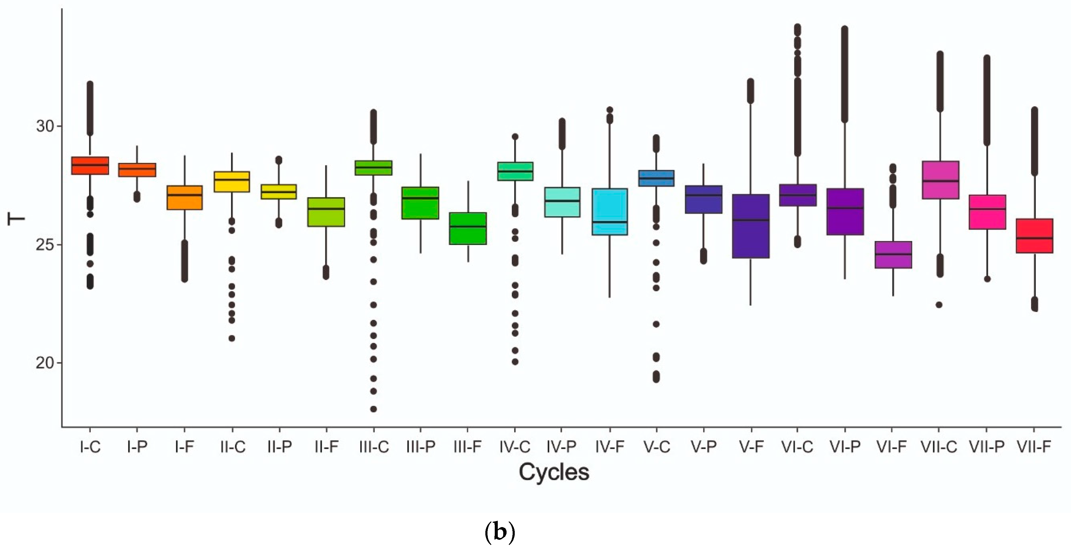
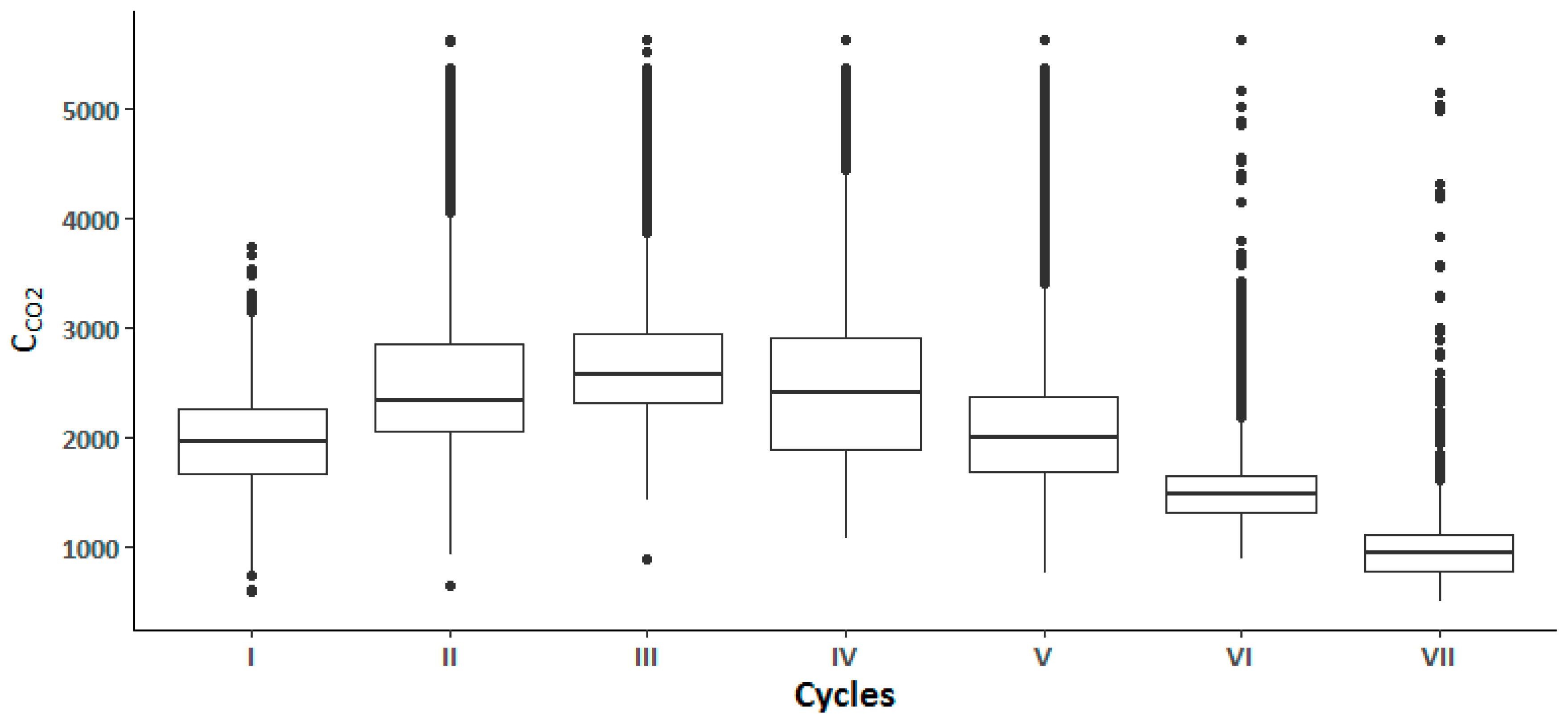
| Cycle | T (°C) | RH (%) | CCO2 (ppm) | ||||||
|---|---|---|---|---|---|---|---|---|---|
| C (SD) | P (SD) | F (SD) | C (SD) | P (SD) | F (SD) | C (SD) | P (SD) | F (SD) | |
| I | 28.5 (0.9) | 28.1 (0.4) | 26.9 (0.8) | 51.9 (9.2) | 54.2 (4.9) | 59.0 (5.0) | 1602.9 (340.8) | 2137.3 (305.9) | 2146.9 (346.8) |
| II | 27.6 (0.6) | 27.2 (0.5) | 26.3 (0.8) | 75.9 (10.8) | 89.2 (17.5) | 100.0 (0.0) | 3021.9 (977.3) | 2369.7 (776.3) | 2598.4 (931.8) |
| III | 28.1 (0.7) | 26.7 (0.8) | 25.7 (0.7) | 100.0 (0.0) | 100.0 (0.0) | 100.0 (0.0) | 3323.8 (1100.1) | 2477.9 (394.2) | 2594.7 (330.9) |
| IV | 28.0 (0.7) | 26.8 (0.9) | 26.4 (1.5) | 100.0 (0.0) | 100.0 (0.0) | 100.0 (0.0) | 3115.4 (890.4) | 2376.9 (504.2) | 1865.1 (491.5) |
| V | 27.8 (0.7) | 26.8 (0.8) | 26.0 (1.9) | 100.0 (0.0) | 100.0 (0.0) | 100.0 (0.0) | 3017.2 (1148.4) | 1973.5 (296.4) | 1587.6 (318.9) |
| VI | 27.2 (1.2) | 26.7 (2.0) | 24.6 (0.9) | 1469.8 (266.2) | 1469.6 (253.4) | 1775.0 (672.2) | |||
| VII | 27.8 (1.7) | 26.6 (1.6) | 25.4 (1.3) | 57.5 (6.2) | 58.4 (6.2) | 64.7 (6.4) | 949.4 (300.5) | 996.0 (264.6) | 995.3 (345.3) |
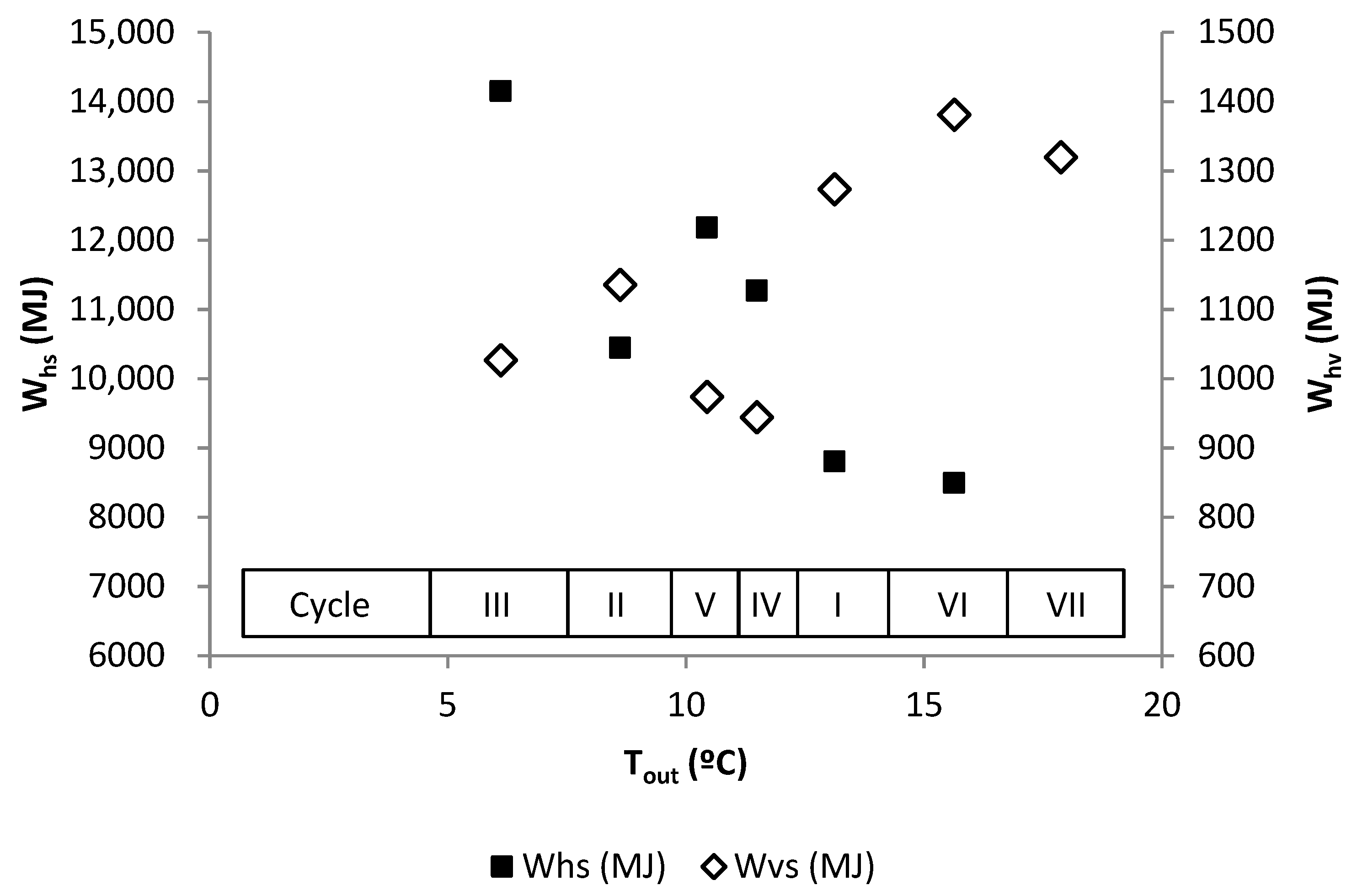
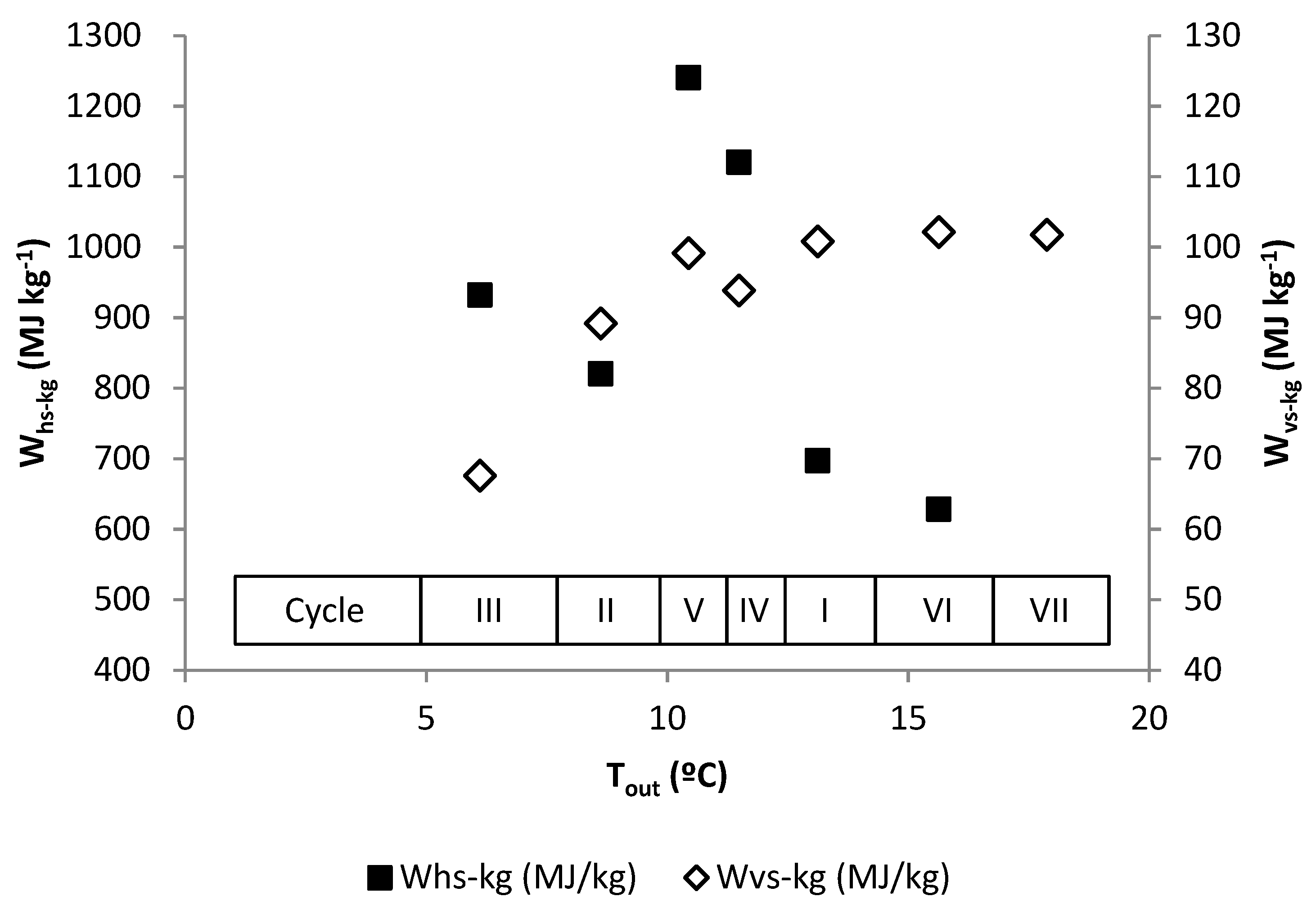
| Tout | RH | CCO2 | Wvs | Whs | |
|---|---|---|---|---|---|
| Tout | 1.00 | 0.55 | 0.91 | 0.54 | 0.75 |
| RH | 1.00 | 0.59 | 0.91 | 0.66 | |
| CCO2 | 1.00 | 0.61 | 0.63 | ||
| Wvs | 1.00 | 0.66 | |||
| Whs | 1.00 |
© 2020 by the authors. Licensee MDPI, Basel, Switzerland. This article is an open access article distributed under the terms and conditions of the Creative Commons Attribution (CC BY) license (http://creativecommons.org/licenses/by/4.0/).
Share and Cite
Fernandez, M.D.; Losada, E.; Ortega, J.A.; Arango, T.; Ginzo-Villamayor, M.J.; Besteiro, R.; Lamosa, S.; Barrasa, M.; Rodriguez, M.R. Energy, Production and Environmental Characteristics of a Conventional Weaned Piglet Farm in North West Spain. Agronomy 2020, 10, 902. https://doi.org/10.3390/agronomy10060902
Fernandez MD, Losada E, Ortega JA, Arango T, Ginzo-Villamayor MJ, Besteiro R, Lamosa S, Barrasa M, Rodriguez MR. Energy, Production and Environmental Characteristics of a Conventional Weaned Piglet Farm in North West Spain. Agronomy. 2020; 10(6):902. https://doi.org/10.3390/agronomy10060902
Chicago/Turabian StyleFernandez, Maria D., Eugenio Losada, Juan A. Ortega, Tamara Arango, María José Ginzo-Villamayor, Roberto Besteiro, Santiago Lamosa, Martín Barrasa, and Manuel R. Rodriguez. 2020. "Energy, Production and Environmental Characteristics of a Conventional Weaned Piglet Farm in North West Spain" Agronomy 10, no. 6: 902. https://doi.org/10.3390/agronomy10060902
APA StyleFernandez, M. D., Losada, E., Ortega, J. A., Arango, T., Ginzo-Villamayor, M. J., Besteiro, R., Lamosa, S., Barrasa, M., & Rodriguez, M. R. (2020). Energy, Production and Environmental Characteristics of a Conventional Weaned Piglet Farm in North West Spain. Agronomy, 10(6), 902. https://doi.org/10.3390/agronomy10060902