Article

A Multiscale Mechanical Model for Plant Tissue Stiffness

1
Department of Mechanical Engineering, McGill University, 817 Sherbrooke St. W., Montreal, QC H3A 0C3, Canada
2
Department of Chemical Engineering, McGill University, 3610 Rue University, Montreal, QC H3A 0C5, Canada
*
Author to whom correspondence should be addressed.
Polymers 2013, 5(2), 730-750; https://doi.org/10.3390/polym5020730
Submission received: 1 April 2013 / Revised: 10 May 2013 / Accepted: 13 May 2013 / Published: 10 June 2013
(This article belongs to the Special Issue Multiscale Simulations in Soft Matter)

Abstract

:
Plant petioles and stems are hierarchical cellular structures, displaying structural features defined at multiple length scales. The current work focuses on the multi-scale modelling of plant tissue, considering two orders of structural hierarchy, cell wall and tissue. The stiffness of plant tissue is largely governed by the geometry of the tissue cells, the composition of the cell wall and the structural properties of its constituents. The cell wall is analogous to a fiber reinforced composite, where the cellulose microfibril (CMF) is the load bearing component. For multilayered cell wall, the microfibril angle (MFA) in the middle layer of the secondary cell wall ( S 2 layer) largely affects the longitudinal stiffness for values up to 40 o . The MFA in turn influences the overall wall stiffness. In this work, the effective stiffness of a model system based on collenchyma cell wall of a dicotyledonous plant, the Rheum rhabarbarum, is computed considering generic MFA and volume fractions. At the cellular level, a 2-D Finite Edge Centroidal Voronoi tessellation (FECVT) has been developed and implemented to generate the non-periodic microstructure of the plant tissue. The effective elastic properties of the cellular tissue are obtained through finite element analysis (FEA) of the Voronoi model coupled with the cell wall properties. The stiffness of the hierarchically modeled tissue is critically important in determining the overall structural properties of plant petioles and stems.

Graphical Abstract

1. Introduction

Plants are one of the major kingdoms in biology. From a structural point of view, a plant exhibits remarkable mechanical properties. Among their organs, the petiole that attaches the leaf to the stem is one of the significant load bearing structures of a plant. As a cantilever beam, the petiole supports the leaf against gravity and allows it to be exposed to the sun. The petiole thus provides mechanical support against the weight of the leaf and against environmental factors, such as rain and wind, resisting both bending and twisting load [1]. The petiole of Rheum rhabarbarum (rhubarb) plant, shown in Figure 1, is an example of a cantilever beam that must resist combined loads including bending and twisting. The petiole’s flexural and torsional stiffness are largely influenced by its overall geometric properties and the stiffness of its constituents, including tissues and cell walls.
Figure 1. Rheum rhabarbarum (rhubarb) plant in a garden (©2000 Rosie Lerner, Purdue University).
Polymers 05 00730 g001
The petiole can be considered as a hierarchical structure, having structural features defined at multiple length scales. A petiole is generally composed of an assembly of cellular tissues whose mechanical characteristics collectively depend on the geometry of their constituent cells, cell wall composition, the structural properties of the wall constituents, and the microstructures of the tissues. It is useful to characterize the structural hierarchies in plants in terms of levels (n). As indicated in Figure 2, n = 1 corresponds to the cell wall, n = 2 to tissue, and n = 3 to the petiole. Although the hierarchical organization of plants spans from the molecular level to the whole organism, in this work the stiffness of tissues is specified by the hierarchies at the cellular and sub-cellular level (Figure 2). Thus, the mechanical attributes of a tissue depend on the structural properties of the cell wall constituents and their structural organizations.
Cell walls are mainly composed of complex networks of polysaccharides, namely cellulose (C), hemicelluloses (HC) and pectin, along with comparatively minor quantities of structural protein and/or lignin [2,3,4,5]. Each Cellulose Microfibril (CMF) is a semi-crystalline aggregate of 36 β-1,4-glucan chains. CMFs are several µm long but only about 3–4 nm thick, and lay 15–30 µm apart in the wall [6]. The construction of the cell wall is considered to be a fiber-reinforced composite, where the cellulose fibrils act as the main load-bearing elements [7,8,9]. The CMFs are embedded in a compliant matrix of hemicelluloses and lignin, where the stiffness of the matrix is approximately two orders of magnitude lower than the CMF [4,10]. Experiments on plant cells show that the properties of CMF strongly dictate the elasticity of the cell wall, while lignin and hemicelluloses have a marginal effect [11]. However, the stiffness of cell wall can be approximated considering the simplest composite model, where the cell wall is a two phase system under uniaxial loading condition [12,13]. Based on the elastic properties and the volume fractions of the CMF and lignin/hemicellulose matrix, the stiffness of the cell wall can be determined for two limiting architectures—parallel (Voigt model) and perpendicular fiber orientations (Reuss model)—with respect to loading direction. Since there is a significant difference in stiffness between the polysaccharides at the cell wall level and other levels of hierarchy, the orientation of the microfibrils in the cell wall influences the stiffness properties of individual cells and tissues as well. The Microfibril Angle (MFA) has been experimentally shown to be a key factor in determining the mechanical properties of plant cell walls [3,4,5,9]. Both experimental and numerical studies show that the structural properties of plants are influenced by the properties of cell wall constituents, MFA and their structural organization [14,15,16]. Hence, the Voigt and Reuss models are insufficient to approximate the stiffness of the cell wall. To determine the longitudinal and transverse modulus, the orthotropic nature of the cell wall should be considered [17,18]. The stiffness of the cell wall should thus be modeled assuming orthotropic material properties, where the constitutive relation yields the stiffness of the cell wall along the orthogonal directions.
Figure 2. Hierarchical organization of Rhubarb petiole. The overall tissue stiffness depends on the stiffness properties of two hierarchical levels: n = 1, and 2. (©US Department of Energy Genome Programs [19].)
Polymers 05 00730 g002
It has been demonstrated that the shape, size, and spatial distribution of cells govern the physical, biological, and structural properties of cellular materials [20,21,22]. Hence, the ability to realistically model the cellular microstructure of a plant tissue is crucial to understanding its mechanical behaviour [23,24]. Many researchers have modeled natural cellular solids using repeating unit cells to construct a regular microstructure in the form of a circular, square or hexagonal array of cells [25]. Closed-form relations of the structure-property can be derived with simplified geometric models based on repeated unit cells [26,27]. Nevertheless, the modeling of plant tissue is a challenging task, since natural cellular solids often exhibit non-periodic arrangement of cells. Since the microstructure is heterogeneous in shape and size, the Voronoi tessellation can be used to generate an accurate representation of a non-periodic microstructure [27,28,29]. Voronoi tessellation is used extensively to model grain geometry for the property characterization of polycrystalline aggregates [30] and inter-granular cracks [31]. Mattea et al. [32] and Roudot et al. [33] pioneered the use of Voronoi tessellation to model the microstructure of fruit tissues. Both groups aimed only to capture the randomness of the fruit tissue microstructure without necessarily producing a model that accurately represented the real tissue. Recently, Ntenga et al. [34,35] tried to analyse the structure, morphology and mechanical properties of the Rhectophyllum camerunense (RC) plant fiber using a conventional Voronoi diagram. Due to inherent drawbacks of the Voronoi (CVT) model, semi-infinite edges were present at the boundary of the fiber, making the model unsuitable for Finite Element Analysis (FEA). To generate a geometric model, having finite edges at the boundary, a Finite-edge Centroidal Voronoi Tessellation (FECVT) method has been developed. The FECVT method has been applied to model the tissue microstructures of emphArabidopsis thaliana and Philodendron melinonii, two plants with distinct tissue architecture [36]. In this work, the FECVT method is applied to generate the virtual model of the rhubarb tissue. Coupled with the cell wall properties, the FEA of the virtual model provides the effective/homogenized tissue stiffness.
Most studies on the homogenization of cellular solids are based on regular models with a periodic microstructure. Real solid foams, however, exhibit amorphous arrangements of pores with different sizes and shapes rather than perfectly periodic structures. The homogenized/apparent elastic property of periodic honeycomb varies from 10% to 15% compared with non-periodic honeycomb [27]. On the other hand, to analyze the irregular microstructures represented by the Voronoi tessellation, the homogenization process requires a large scale representative volume element (RVE). Analyses of such models had been provided, among others, by Silva et al. [27], Fazekas et al. [37], Roberts and Garboczi [38] for both two and three-dimensional models. To obtain the homogenized/effective stiffness properties, the 2-D virtual tissue (RVE) undergoes FEA for a given boundary condition [39]. The computational homogenization technique is used with non-periodic microstructure for global homogenization. This technique can effectively consider the microstructural irregularity present in the plant tissues. The effective properties can be used in the next hierarchical level to capture macro-scale properties such as bending and torsional stiffness of the whole petiole.
The objective of this work is to determine the theoretical bounds of stiffness of the collenchyma tissue modeled with two orders of structural hierarchy, namely cell wall and tissue micro-architecture. At the first order of the hierarchy, the constitutive properties of the cell wall are modeled via the classical micromechanical models of Voigt and Reuss, and the microfibril angle. The geometric model of the collenchyma tissue is generated by the FECVT algorithm; it undergoes finite element analysis that accounts for the cell wall properties to determine the stiffness of the tissue at the second order of the hierarchy.

2. Methodology

Since most plant tissues display hierarchical organization, we adopt in this work a hierarchical modeling approach to obtain their stiffness properties. In the first order of the hierarchy, the cell wall stiffness is modeled considering as variables the MFA and the volume fractions of the wall constituents, and their elastic properties. The obtained wall stiffness is then used in the next hierarchical level, where the effective stiffness of tissue, represented by an FECVT model, is determined through FEA.

2.1. Stiffness of Cell Wall via Micromechanics Theory

The cell wall, which belong to the bottommost hierarchy (n = 1 in Figure 2), is the building block at this level of hierarchy. The upper and lower limits of stiffness of the cell wall can be determined using micromechanical models—Voigt and Reuss models. Three pieces of information are required in the model: (i) the elastic moduli of cell wall constituents; (ii) the volume fractions of the various constituents; and (iii) the geometric arrangements of the constituents relative to each other. The properties of the cell wall constituents are available in literature. For example for cellulose, a wide range of theoretical as well as experimental estimation of its elastic modulus is reported. Earlier theoretical prediction of Young’s modulus provides relatively higher values, 246 and 319 GPa [40,41], whereas more recent analyses show 120–140 GPa [42,43,44] and 167 GPa [45] for crystalline cellulose along the fiber direction. Data for the elastic modulus of hemicelluloses are scarce and fall within a range of 5–8 GPa [46]. The elastic properties of lignin are difficult to assess and vary from 4 to 7 GPa [47,48]. Considering an orthotropic arrangement in the cell wall, a set of rational moduli [10] used in this work are shown in Table 1. The volume fractions and the geometric arrangements of the constituents are discussed in Section 3.1, where their effects on the engineering properties of cell wall are discussed in detail.
Table 1. Elastic properties of cell wall constituents used in the present work [10].
PropertiesCMFLigninHemicellulose
E x (GPa)1342.02.0
G (GPa)4.41.00.6
ν0.10.20.3
Note: Dry conditions (12% moisture), 20 °C.
The values shown in Table 1 are used in the Voigt and Reuss models to determine the wall stiffness along the fiber direction, E 1 , and across the fiber direction, E 2 (Figure 3). The Voigt upper bound is
E 1 = E f v f + E m v m
and the Reuss lower bound is
1 E 2 = v f E f + v m E m
where E 1 and E 2 refer to the Young’s moduli of the composite, E f and E m refer to the Young’s modulus of fiber and matrix, respectively; v f and v m refer to the volume fraction of fiber and matrix, respectively, with v f + v m = 1 .
Using the same concept, the major Poisson’s ratio, ν 12 , along the fiber direction, is
ν 12 = ν f v f + ν m 1 - v f
Figure 3. Voigt and Reuss models.
Polymers 05 00730 g003
and the minor Poisson’s ratio, ν 21 , across the fiber direction, can be derived with the reciprocal relationship
ν 21 E 2 = ν 12 E 1
The in-plane shear modulus can be expressed as
G 12 = G m G f G f 1 - v f + G m v f
However, an actual cell wall may not behave according to the predictions based on either the pure Reuss or the pure Voigt model. Rather, a hybrid model appears to be the best modeling approach although the Voigt elements appear to be dominant.

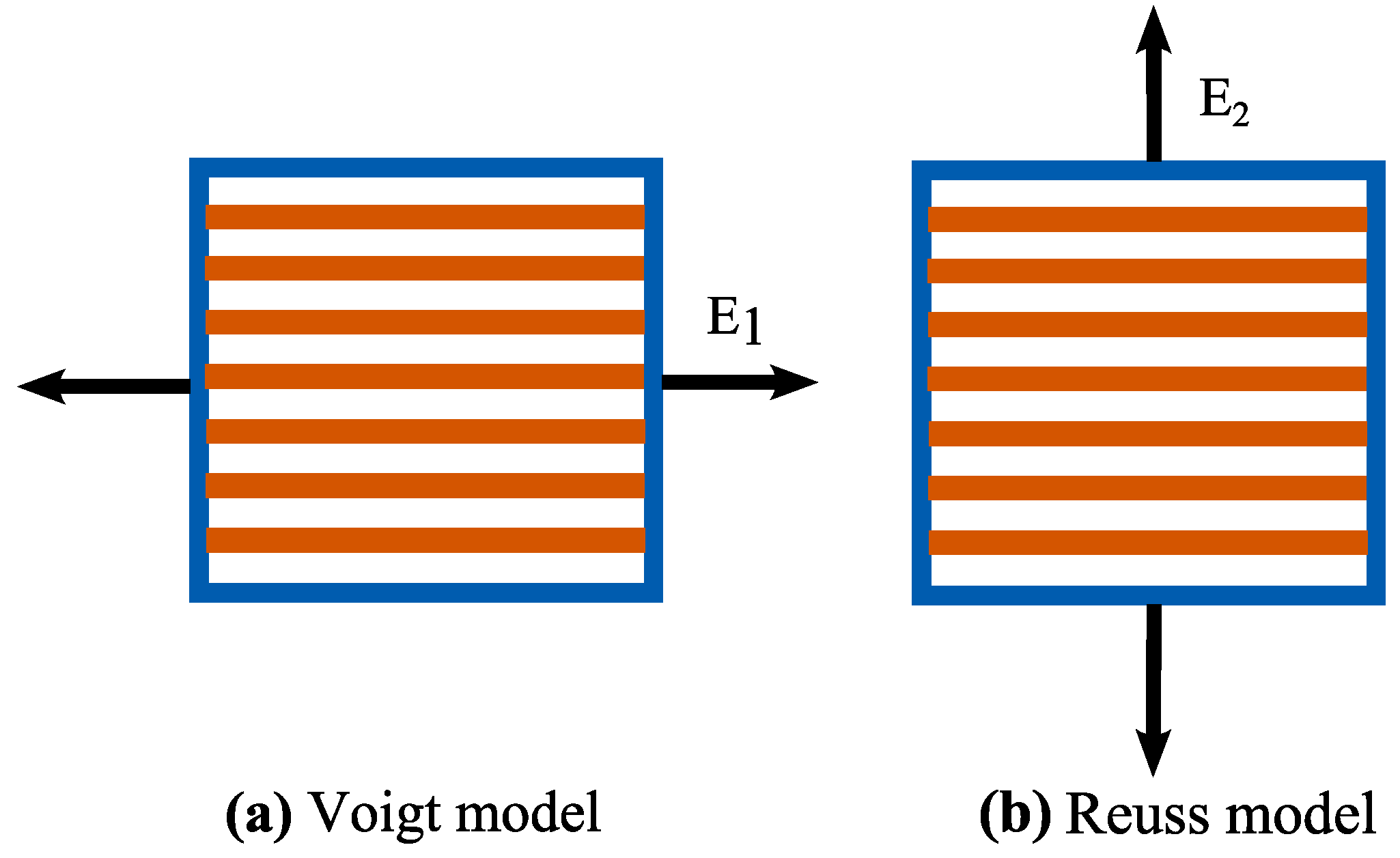
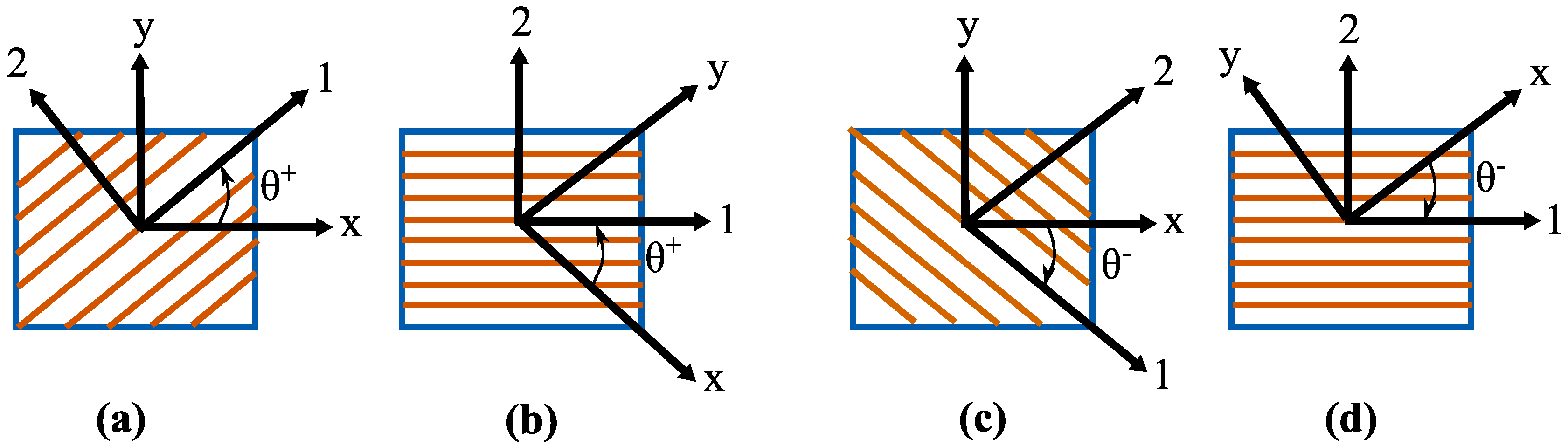
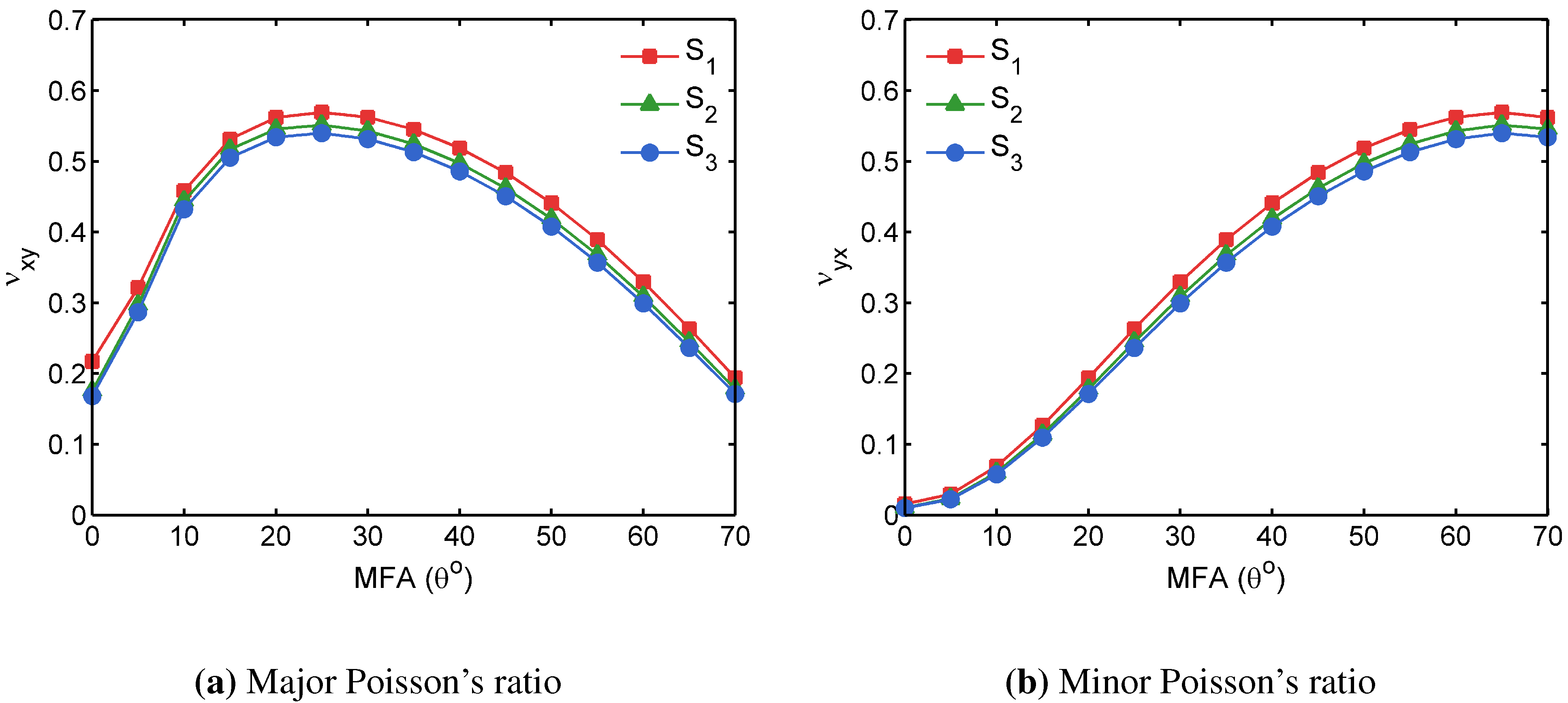
2.2. Constitutive Properties of Cell Wall using Macromechanics

The constitutive relation for the CMF (fiber) reinforced cell wall depicts the stiffness in the global coordinate system. For an orthotropic cell wall, the compliance matrix is expressed for plane stress condition as
[ S ] = S 11 S 12 0 S 12 S 22 0 0 0 S 66
where
S 11 = 1 E 1 , S 12 = - ν 21 E 2 = - ν 12 E 1 = S 21 , S 22 = 1 E 2 , S 66 = 1 G 12
The constitutive relation for an orthotropic material is therefore,
{ ϵ } = [ S ] { σ } = [ Q ] - 1 { σ }
where [ Q ] is the stiffness matrix, [ S ] is the compliance matrix with [ S ] = [ Q ] - 1 .
Equation (7) stands for the on-axis configuration, where the global coordinate system, x-y axis, coincides with the local coordinate system, 1-2 axis, respectively. When the local and global coordinates do not coincide, the arrangement is the off-axis configuration, shown in Figure 4. Therefore, the on-axis stress-strain relationship is not adequate for the analysis of an off-axis configuration. In the off-axis configuration, the stiffness depends on the fiber orientation angle, which is termed as the MFA for the cell wall configuration. Thus, the MFA needs to be addressed in the constitutive relation. If the x-y coordinate system is aligned with the direction of loading and the 1-2 coordinate system is aligned with the fibers, MFA (θ) is the angle between the two (Figure 4).
The local (1-2) and global (x-y) coordinate systems are related through a transformation equation. Hence, the transformation of strains between the loading (local) direction and the fiber (global) direction is denoted by
ϵ 1 ϵ 2 ϵ 6 = m 2 n 2 m n n 2 m 2 - m n - 2 m n 2 m n m 2 - n 2 ϵ x ϵ y γ x y = [ T ϵ ] ϵ x ϵ y γ x y
where m = c o s θ , m = s i n θ and [ T ϵ ] is the strain transformation matrix. Similarly, the stress transformation matrix is
σ 1 σ 2 σ 6 = m 2 n 2 2 m n n 2 m 2 - 2 m n - m n m n m 2 - n 2 σ x σ y τ x y = [ T σ ] σ x σ y τ x y
Figure 4. On-axis and off-axis configurations.
Polymers 05 00730 g004
Reorganizing and combining Equations (7)–(9), the Cartesian strain-stress relationship in the global coordinate system is given by
ϵ x ϵ y ϵ x y = [ T ϵ ] - 1 [ S ] [ T σ ] σ x σ y τ x y = [ S ¯ ] σ x σ y τ x y
where [ S ¯ ] is a new matrix known as the transformed reduced compliance matrix. The off-axis constitutive relationship can be expressed in the following form:
ϵ x ϵ y γ x y = S ¯ 11 S ¯ 12 S ¯ 16 S ¯ 12 S ¯ 22 S ¯ 26 S ¯ 16 S ¯ 26 S ¯ 66 σ x σ y τ x y
In summary, the constitutive (engineering) properties of cell wall are
E x = E 1 m 4 + E 1 G 12 - 2 ν 12 n 2 m 2 + E 1 E 2 n 4
ν x y = ν 12 n 4 + m 4 - 1 + E 1 E 2 - E 1 G 12 n 2 m 2 m 4 + E 1 G 12 - 2 ν 12 n 2 m 2 + E 1 E 2 n 4
E y = E 2 m 4 + E 2 G 12 - 2 ν 21 n 2 m 2 + E 2 E 1 n 4
ν y x = ν 21 n 4 + m 4 - 1 + E 2 E 1 - E 2 G 12 n 2 m 2 m 4 + E 2 G 12 - 2 ν 21 n 2 m 2 + E 2 E 1 n 4
G x y = G 12 n 4 + m 4 + 2 2 G 12 E 1 1 + 2 ν 12 + 2 G 12 E 2 - 1 n 2 m 2

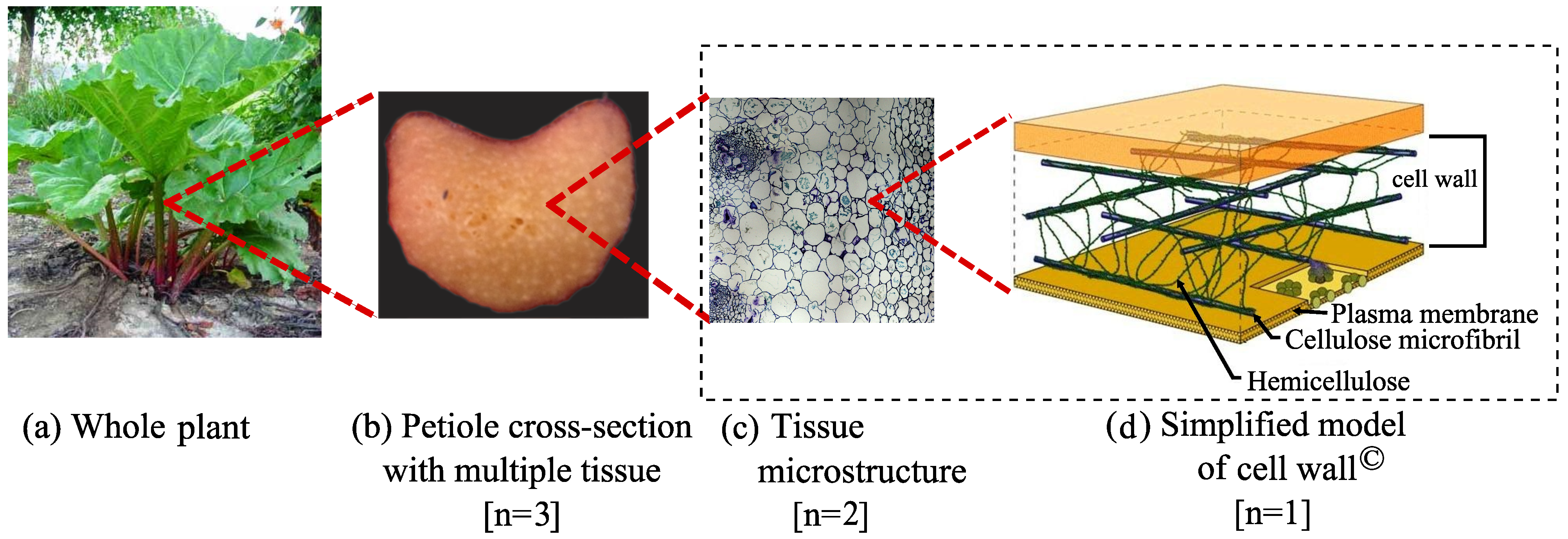
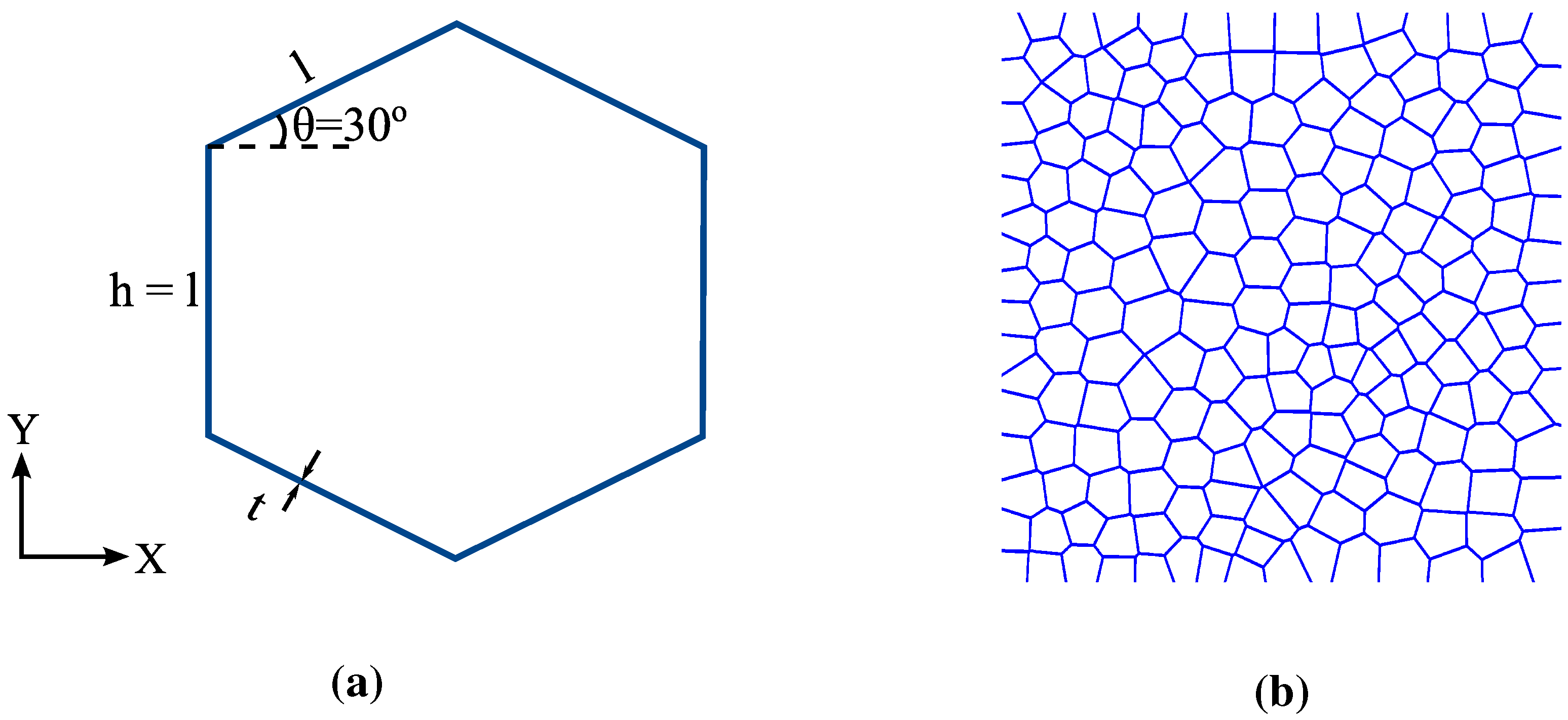
2.3. Geometric Modeling

A Voronoi microstructure is constructed based on a set of randomly generated points called Voronoi sites. The cell boundaries are drawn such that any point within the enclosed polygon is closer to its Voronoi site than to the Voronoi sites of the surrounding polygons. The Voronoi tessellation thus divides a space into as many regions as there are Voronoi sites. In the current method, the centroids of the cells are used to construct the Voronoi diagram. To construct a centroidal Voronoi tessellation (CVT), first, a color or greyscale micrograph of a plant tissue is subjected to image segmentation. Thresholding, a method for image segmentation, converts the color or greyscale image into a binary (black and white) image. Since plant tissues usually exhibit graded cellularity as well as complex heterogeneity, an edge detection algorithm is used in conjunction with thresholding to obtain the cellular distribution accurately. The Canny edge detection algorithm [49] is used here to detect the shapes of the cells more precisely.
Once the shapes of the cells are detected, the first order moments of the cells are computed using X and Y coordinates of the pixels. The algebraic form of the moment equation of a digital image is
m p q = i = 1 n 1 j = 1 n 2 X i p Y j q f i , j
where X i , Y j is the coordinate of the ( i , j ) t h pixel, f i , j have value 1 if the ( i , j ) t h pixel is in the shape and 0 otherwise. Considering the region of interest, which is completely enclosed in a rectangular region G of size n 1 by n 2 pixels, i varies from 1 to n 1 , and j varies from 1 to n 2 in the function f i , j . For a 2-D region, p + q denotes the order of moment, where p and q are integers. Hence, the coordinates of a cell are
X ¯ = m 10 m 00 and Y ¯ = m 01 m 00
where the zeroth moment, physically, is equal to the area of the region.
After determining the centroids of the cells, the Voronoi tessellation is constructed based on the Quick hull algorithm [50]. The outcome is a conventional CVT with semi-infinite edges at the boundary. The semi-infinite edges complicate finite element analysis because the boundary conditions, applied at an infinite distance, are not realistic. This problem is especially difficult to correct in models with irregular shape contour.
To remove the infinite edges from the boundary, the centroids of the outermost cells are determined. For each centroid, the distances between the centroid and the surrounding Voronoi sites (centroids of the surrounding polygons) are calculated, and the minimum distance is determined. An imaginary point is created such that the distance between itself and the centroid is half of the minimum distance. The imaginary point is thus created for each of the selected centroid. Based on the set of imaginary points and the convex hull algorithm [50], a boundary is imposed, after which a Boolean subtraction is realized. With this Boolean operation, the semi-infinite edges are truncated, and the vertices of the truncated edges are reconnected to form the final boundary. The FECVT technique is, therefore, capable of capturing the microstructure of an image with an arbitrarily shaped boundary contour. This novel computational algorithm, FECVT method [36], is applied here to model the rhubarb tissue microstructure.

2.4. Finite Element (FE) Modeling

The compressive stress-strain regime of the Voronoi microstructure is determined using finite element analysis (ANSYS Inc., Canonsburg, PA, USA). Each cell wall of the Voronoi microstructure is modeled with a BEAM23 element, capable of modeling both elastic and plastic behaviour. The shear deformation, which is important for stubby beam, is also captured by considering the shear deflection coefficient of the beam element. Beams have a rectangular cross-section of uniform thickness, t. The relative density ρ * / ρ s of the microstructure is given by
ρ * ρ s = a r e a o f s o l i d w a l l s t o t a l a r e a o f a V o r o n o i m o d e l = t i = 1 N l i L X L Y
where N is the total number of beams, l i is the length of the beam i; L X and L Y are the dimensions of the Voronoi model along X and Y directions, respectively. The FEA is conducted for different relative density, adjusted by the value of t. In the finite element analysis, a Young’s modulus E s = 1 is assigned to each beam to obtain the normalized tissue stiffness.

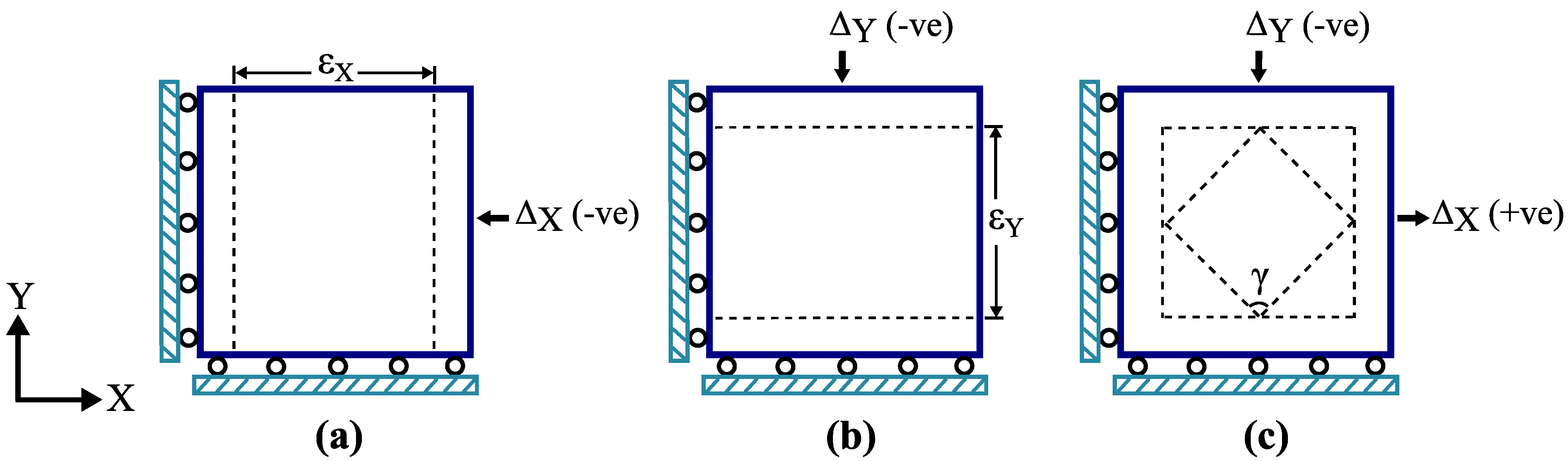
2.4.1. Boundary Conditions

Three types of boundary conditions (BC)—(1) mixed boundary condition, (2) prescribed displacement boundary condition, and (3) periodic boundary condition—can be generally imposed. Since the microstructure is not periodic, the periodic boundary condition is not appropriate here. The mixed boundary condition enforces the normal displacement, eliminating the tangential force and the bending moments at the nodes on the boundaries. Since the mixed boundary condition tends to underestimate the Young’s modulus [51], the displacement boundary condition has been selected, which has been proved to be appropriate for the analysis of non-periodic microstructures for uniaxial and biaxial loading cases [27,29,37,52].
To determine the effective Young’s modulus, uniaxial compression load with prescribed displacement is simulated. A uniaxial compressive strain along the X axis is imposed on the nodes of the right edge while the nodes at the left edge are constrained from translating in this direction (Figure 5). The nodes of the bottom edge are also constrained from translating in the Y direction to prevent the rigid body motion. Similarly, uniaxial compression along Y axis has also been performed. In both cases, nodes are constrained from rotating in the X - Y plane. To determine the effective shear modulus, a biaxial loading test is simulated with a positive displacement in the X direction and a negative displacement in Y direction. The results are computed for alternative values of densities for prescribed boundary conditions.
Figure 5. Simulated test for determining the effective stiffness properties.
Polymers 05 00730 g005

2.4.2. Determination of Apparent Tissue Stiffness

For each model with a given relative density, the effective Young’s modulus, E * , and effective shear modulus, G X Y * , are determined. The macroscopic stress, σ * , is calculated from the global reaction forces of the structure in the loading direction. The sum of the nodal reaction forces is divided by the edge length to determine the normal stress in the loading direction. The strain, ϵ * , is determined based on the technique of gage lines introduced by Silva [27] to eliminate the end effects. The shear strain is computed as the change in the angle between the gage lines oriented at 45 ° , with respect to the coordinate axes.

3. Results and Discussion

The multiscale hierarchical approach can be applied effectively to simulate the stiffness of various plant tissues. In the present work, the method is implemented to the collenchyma tissue of a dicotyledonous plant organ, the rhubarb petiole.

3.1. Stiffness of Cell Wall

The properties of a cell wall depend on the wall constituents, mainly cellulose microfibril, lignin, and hemicellulose. The CMF of cellulose acts as the load bearing element that controls the wall properties. Along with the elastic properties of the constituents (shown in Table 1), the volume fractions of the constituents play an important role as well. The volume fractions of the constituents are not homogenous throughout a multilayered plant cell wall. The layered construction is usually evident in woody plants but is also observed in many other plants. Although the number of layers depends on several factors, such as the types of species, cells, the cell wall is widely accepted to be considered as a three-layered structure. In fact, the woody plants typically exhibit three secondary layers along with a primary layer and middle lamellae. The primary layer only plays a significant role in the early stage of a growing plant. When a plant cell reaches its maturity, the secondary wall becomes the determinant governing its mechanical performance. The volume fractions of CMF, lignin, and hemicelluloses shown in Table 2 represent values of a typical set of multilayered plant cell walls. However, the composition of the constituents depends on other factors as well, such as types of species, and cells, location of the cells and the age of a plant.
Table 2. Approximate volume fractions of tracheid cell wall [41].
Cell wall layerCMF (%)Lignin (%)Hemicellulose (%)
S 1 284527
S 2 452035
S 3 471538
The data shown in Table 1 and Table 2 are used to compute the effective engineering properties, such as stiffness and Poisson’s ratio, of cell wall. The variations of stiffness with respect to MFA along different layers are shown in Figure 6. Figure 6a depicts the effect of MFA on longitudinal the Young’s modulus for each layer. Up to 40 ° , the effect of MFA on the longitudinal wall stiffness is substantial, and the stiffness is reduced to a considerable amount. In contrast, the transverse stiffness is nearly invariant with the MFA up to 50 ° . Beyond this limit, the transverse modulus varies with MFA and increases with the increasing MFA. The shear modulus is maximum for CMF equal to 45 ° in the loading direction. However, the variation of shear modulus up to 20 ° is less significant, and a gradual increase is observed until the MFA reaches 45 ° and starts decreasing afterwards. The Poisson’s ratios shown in Figure 7 vary with the MFA. From the comparison of the minor Poisson’s ratio, we observe that the major Poisson’s ratio increases rapidly up to MFA of 20 ° . The major Poisson’s ratio plays an important role in influencing the anisotropic cell wall properties.
It is evident that the MFA plays a significant role in the wall stiffness, an observation that has been experimentally noticed in numerous plants’ cell wall. The MFA usually varies between 0 ° and 40 ° , in the S 2 layer [53,54,55] and plays a leading role in determining the overall wall stiffness. Moreover, since the thickness of S 2 layer is generally much higher than that of S 1 and S 3 (also primary layer) layers, the measurement of MFA for the whole cell wall or the average MFA across the cell wall involves the approximation of MFA in the S 2 layer. Thus, the S 2 layer is often the main determinant of the stiffness of plant [56]. This concept is used here to determine the effective engineering properties of a single layered dicotyledonous cell. Although a more accurate and rigorous analysis would be conceivable considering microfibril angles at different layers, the composition of S 2 layer with respective MFA provides a good approximation for the overall stiffness of cell wall. Moreover, the measurement of microfibril angles in different layers is not always experimentally possible. Since the focus of this paper is to develop a multiscale model that accounts for the elastic part of the deformation, the nonlinear mechanical response has been ignored. Yet, the non-linear response of plant tissue is important because the approach presented here can be extended to model the nonlinear deformation of the cell wall as well.
Figure 6. Stiffness properties of different cell wall layers for varying MFA.
Polymers 05 00730 g006
In stems and petioles, collenchyma tissue is observed in peripheral locations, beneath the epidermal layer (Figure 8). As per experimental measurements, the collenchyma tissue typically comprises 20% cellulose and the rest 80% of HC and lignin [57,58]. Although there is no clear distinction, the collenchyma cell walls can be considered to be secondary cell wall [58,59], where the orientation of CMF is mostly found to be inclined to the longitudinal axis [60,61,62,63,64,65]. However, the MFA also varies with the technique used for the measurement. For dicotyledonous plants, the MFA usually lies between 6 ° and 15 ° [66]. Based on the fiber volume fraction and MFA, the stiffness of collenchyma tissue is derived. The effective stiffness properties of collenchyma cell wall with 15 ° MFA are summarized in Table 3. The effective stiffness of the collenchyma tissue will be determined based on the effective wall stiffness.

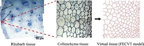
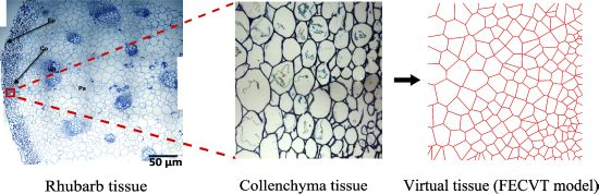
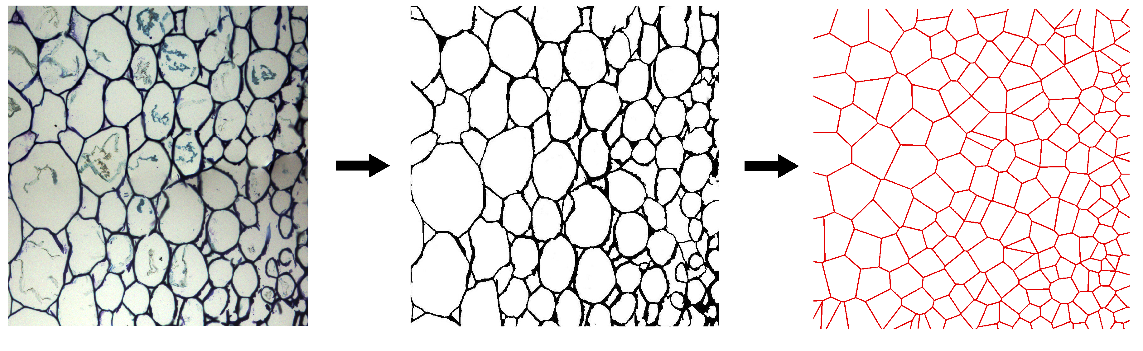
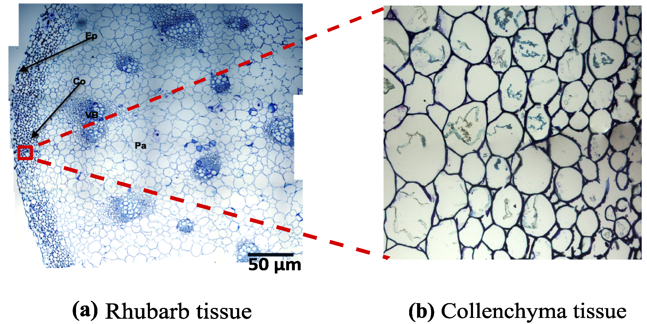
3.2. FECVT Modeling of the Tissue Microstructure

The geometry of the collenchyma tissue of the rhubarb petiole is generated using the FECVT algorithm. Figure 9 shows the collenchyma tissue and its corresponding FECVT model. The latter is obtained with a method recently introduced to represent complex geometric heterogeneity in plant tissue [36]. Since experimental data are used to formulate the mathematical model, the accuracy of the model appears to depend on the quality of the micrograph. The FECVT method, thus, can capture the details of a cellular distribution if the micrograph of the tissue microstructure is vivid and clear. If a conventional CVT were to be used, the reproduction of the polygons at the boundary would differ for their shape and size from those obtained with a FECVT.
Figure 7. Major Poisson’s ratio of different cell wall layers for varying MFA.
Polymers 05 00730 g007
Figure 8. Paraffin-embedded rhubarb petiole cross-section stained with TBO and imaged with light microscopy at 20× magnifications. Approximately 16 photos were stitched together to create this composite image. Ep-epithelium, Co-collenchyma cells, VB-vascular bundle, Pa-parenchyma cells are visible. Scale bar = 50 µm. (b) An enlarged view of a section of collenchyma tissue.
Polymers 05 00730 g008
FECVT models are generated for several arbitrarily chosen sections of collenchyma tissue. Each section is a representative of the respective tissue. Nonetheless, a one-way ANOVA is used to test the differences of FECVT models generated for the tissue and shown in Table 4. The first column in Table 4 corresponds to the between-groups and within-groups estimate of variance, which are shown in the fourth column, showing the mean square. The second column gives the sum of squares for each of the estimates of the variance. The third column gives the degrees of freedom (df) for each estimate of the variance. The number of FECVT models and the sum of the Voronoi cells in the models are used to calculate the degrees of freedom between-groups and within-groups, respectively. The fifth column, F, corresponds to the ratio of the variance of between-groups and within-groups, shown in the preceding column. The last column gives the probability of significance of the F ratio, i.e. p value. Since the p value is greater than the significance level ( α = 0 . 05 ), the null hypothesis is not rejected. Therefore, the FECVT models statistically do not differ significantly across the models as determined by one-way ANOVA ( F ( 2 , 611 ) = 0 . 172 p = 0 . 837 > 0 . 05 ). The output of the ANOVA test implies that the FECVT models of the stochastically chosen collenchyma tissue sections are statistically invariant; hence each model can be considered to be a representative volume element for the FEA.
Table 3. Stiffness properties of collenchyma cell wall determined via Equations (12)–(16).
E x (GPA) E y (GPA) G x y (GPA) ν x y ν y x
Cell wall11.8342.4891.3390.36800.0774
Figure 9. FECVT Model of the collenchyma tissue of rhubarb petiole with intermediate grey scale image.
Polymers 05 00730 g009
Table 4. ANOVA for the FECVT models of collenchyma tissue.
  Sum of squares df Mean square F Sig.
Between Groups 0.651 2 0.321 0.172 0.837
Within Groups 1146.397603 1.863 – –
Total 1147.058605 – – –

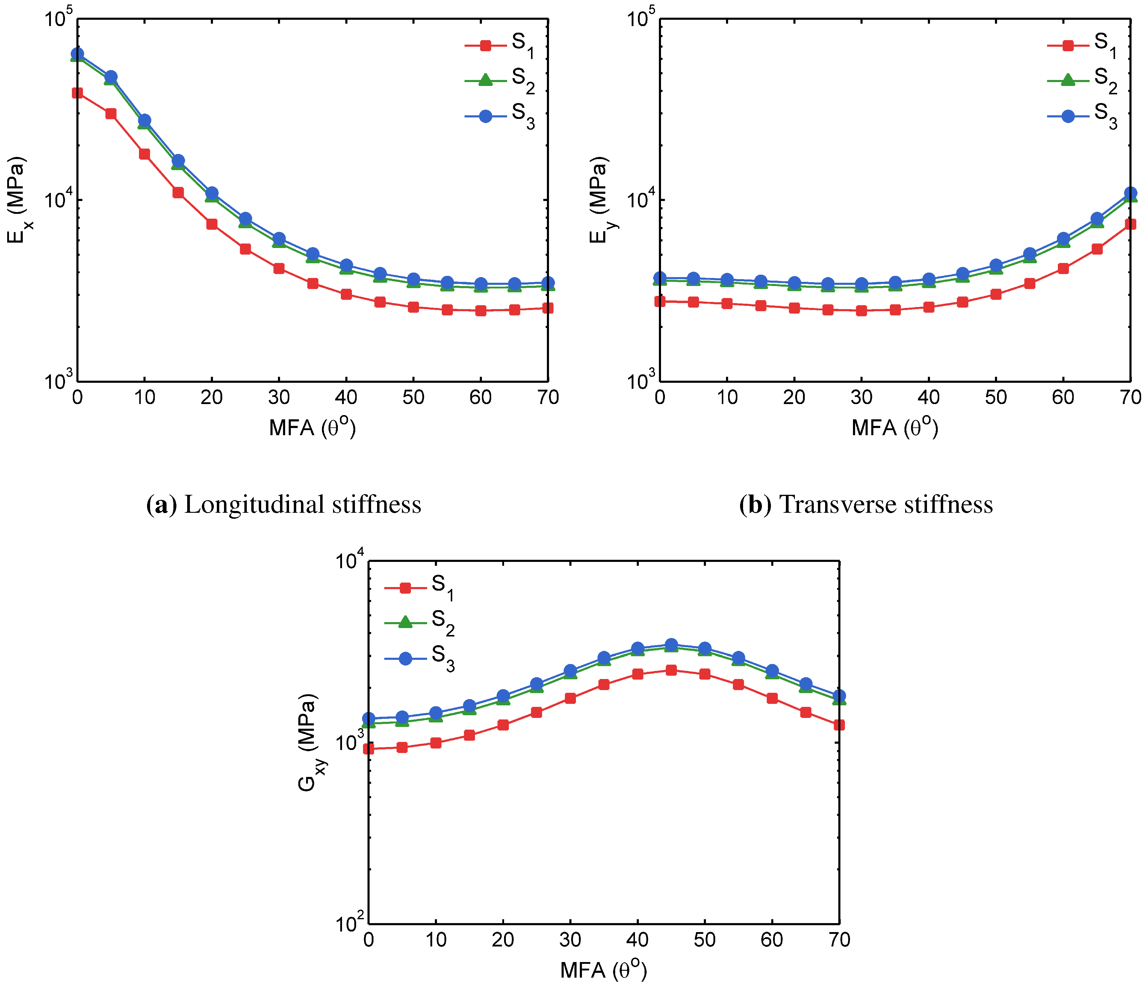
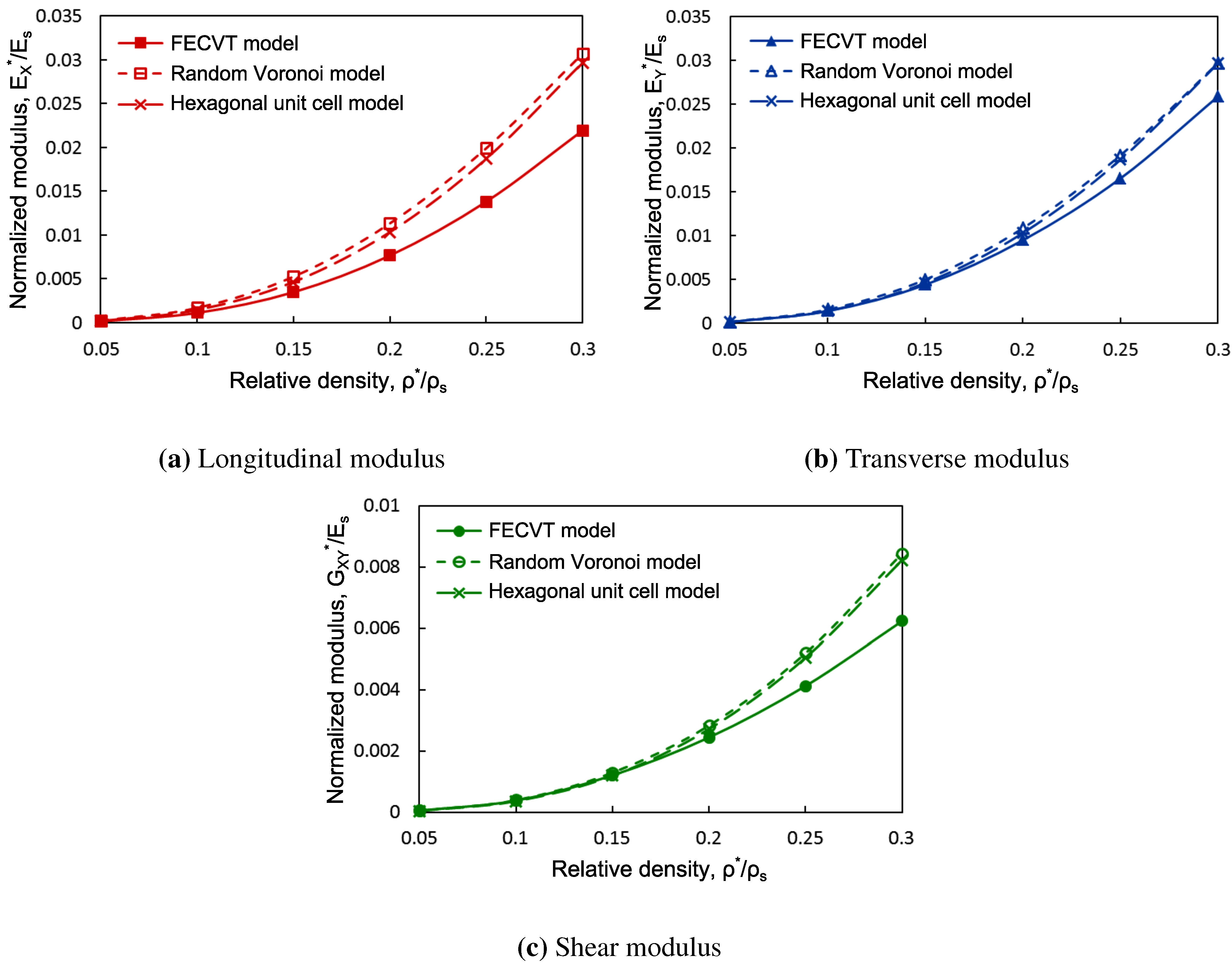
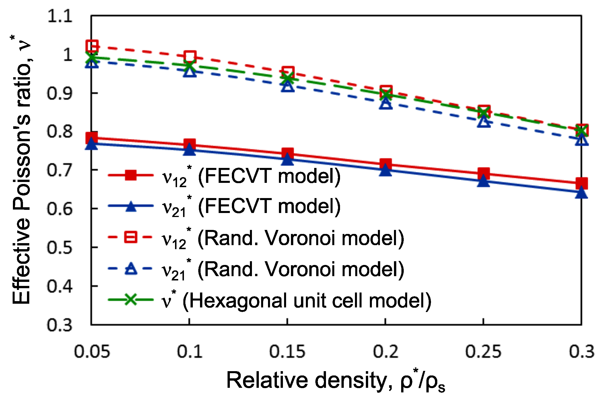
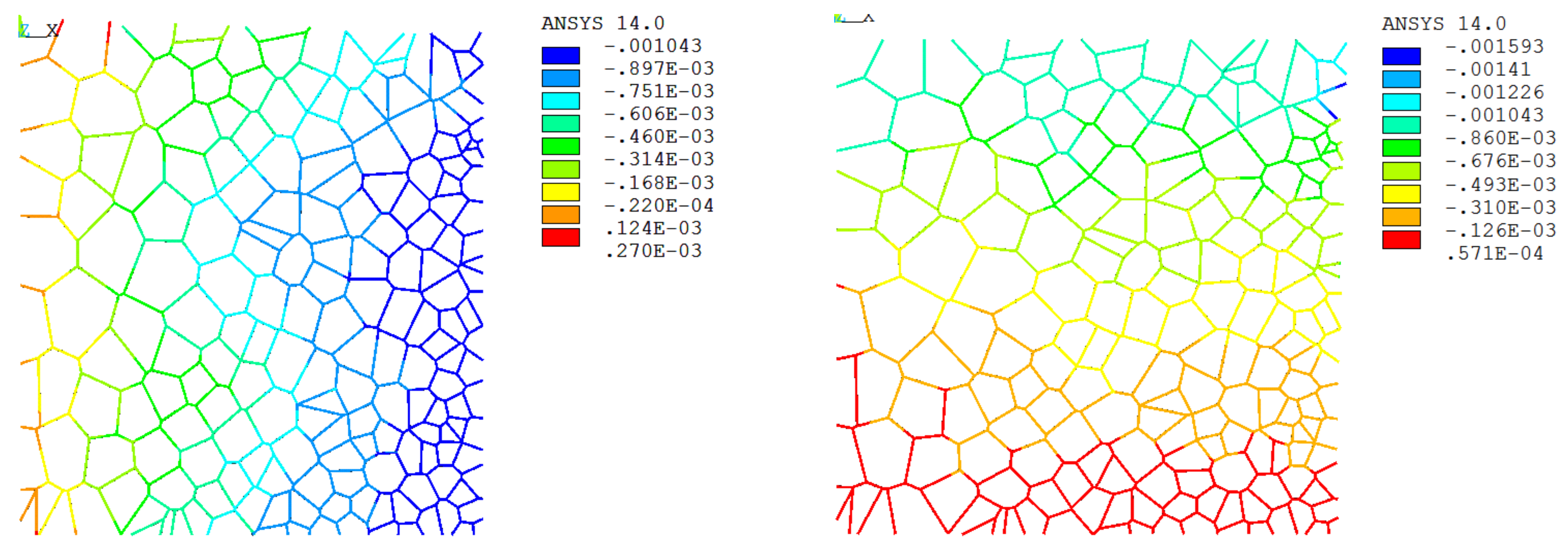
3.3. Apparent Tissue Stiffness through FEA

The FECVT model captures the cellularity present in the tissue microstructure, which in turn is used in the finite element analysis. In a conventional Voronoi model, the boundary cell areas are large because of semi-infinite edges. Hence, the areas of the virtual cells differ significantly with respect to the original images. The FECVT models of the selected collenchyma sections are simulated in ANSYS to determine the effective tissue stiffness. Figure 10 shows the nodal displacements of model tissue for 15% relative density with compressive strain along X and Y directions. The microstructure in X direction is less stiff than that in the Y direction. The microstructural anisotropy of the plant tissue originates from the cellular distribution.
We have compared the normalized stiffness obtained with the FEA of the FECVT model with the stiffness of a randomly generated Voronoi model, and the stiffness calculated from closed-form expressions available in literature [27]. These formulas are obtained with an isotropic periodic cellular model having a hexagon as unit cell. On the other hand, the random Voronoi model is generated for a set of uniformly distributed points. Both the FECVT and randomly generated Voronoi models have the same number of cells. Figure 11 shows a regular hexagonal unit cell and the randomly generated Voronoi model.
Figure 10. Nodal displacement of FECVT model under uniaxial displacement boundary condition: (a) X component of nodal displacement; (b) Y component of nodal displacement.
Polymers 05 00730 g010
Figure 11. (a) Hexagonal unit cell; (b) Randomly generated Voronoi model for a set of 196 uniformly distributed points.
Polymers 05 00730 g011
Both the randomly generated Voronoi and FECVT models are simulated for a set of relative densities between 5% and 30%. The normalized effective stiffness of both the models and the hexagonal unit cell are shown in Figure 12. The FEA of the random Voronoi model shows an average of 8% and 6% higher axial and shear modulus, respectively, compared with the closed-form solutions obtained for the unit cell shown in Figure 12. The results of the moduli are in agreement with those presented by Gibson et al. [26,27]. For given relative density, the normalized effective elastic moduli of the different models in X and Y direction are shown in Figure 12. For relative density, 0 . 05 ρ * / ρ s 0 . 30 , the FECVT model is 54% to 40% less stiff than the randomly generated Voronoi model and 31% to 35% less stiff than the periodic unit cell along the direction. Along the direction, the FECVT model is 19% to 15% less stiff than the random Voronoi model and 1% to 14% less stiff than the unit cell model for relative densities varying between 5% and 30%. To generate the Voronoi tessellation, we impose a uniform distribution of points. Hence, the randomly generated Voronoi model displays a uniform cell size, a factor that influences the stiffness properties, as shown in Figure 12. In the FECVT model, both shape and size of the cells vary significantly with respect to the random Voronoi model and the hexagonal cell model. Therefore, the shape and size of the cells affect the normalized stiffness, which varies with density. Similarly, the shear modulus of the FECVT model is lower than both the random Voronoi model and the unit cell model.
Figure 12. Normalized elastic modulus as a function of relative density.
Polymers 05 00730 g012
The normalized effective stiffness of the FECVT model along the longitudinal direction is around 15% to 25% higher than that of the FECVT model along transverse direction for the range of density considered here. The variation reflects the stiffening effect of the cell shape, size, and the cellular distribution. It also depicts the anisotropic behaviour of the collenchyma tissue of the rhubarb petiole. Since the FECVT model contains smaller cells than those of the actual tissue, the stiffness could be overestimated. In addition, the short cell walls modeled by the beam element may impose superfluous stiffness. Figure 13 depicts the effective Poisson’s ratios for the FECVT, random Voronoi, and hexagonal unit cell models. The finite element analyses of both the FECVT and random Voronoi models exhibit marginal difference between the major and minor Poisson’s ratio. Because of uniform cellular distribution, the Poisson’s ratios of the random Voronoi model depend weakly on relative density. Hence, the microarchitecture of the tissue also affects the Poisson’s ratio.
The effective stiffness of the cellular tissue can be obtained based on the computed wall stiffness in the previous hierarchy. For a relative density of 15%, the effective stiffness of the collenchyma tissue is 41.1 MPa and 11.02 MPa along X and Y direction, respectively. Instead of generic composition of dicotyledonous plant cell wall, the volume fractions and MFA of the model plant should be determined experimentally, and the computational stiffness would be more representative of and closer to the actual tissue stiffness. Moreover, the model is simplified, ignoring the presence of multilayers, if any. Despite the limitations, the approach is able to capture the stiffness at different hierarchical orders and the overall effective stiffness of the hierarchical cellular tissue.
Figure 13. Effective Poisson’s ratios as a function of relative density.
Polymers 05 00730 g013

4. Conclusions

Cellular solids are prevalent both in nature and in man-made engineering structures. Their microstructures govern the mechanical response at the macroscale. A micromechanical analysis that captures the realistic arrangement of the microstructure can thus provide insight into the overall macroscale behaviour of a cellular material. The goal of this work is to develop a multiscale hierarchical methodology to determine the stiffness of cellular plant tissue. In this paper, the stiffness properties at two orders of the tissue hierarchy have been determined by modeling structural details at their respective length scales. The upper and lower bounds of stiffness of the cell wall have been approximated via the classical micromechanical models of Voigt and Reuss. The microfibril angle and the stiffness bounds at the sub-cellular level have been used to compute the effective stiffness of the cell wall. We have shown that the MFA of the S 2 layer influences the overall stiffness of a multilayered secondary cell wall. The effect of MFA on the stiffness properties of single layered collenchyma cell wall of rhubarb petiole has also been captured at this order of hierarchy. The MFA governs the stiffness properties of both single and multilayered cell wall. At the cellular level, the tissue has been realistically modeled with the FECVT algorithm, which is capable of representing the actual cell distributions within the collenchyma tissue. The geometric model is representative of the cellular tissue and allows to numerically obtain the elastic properties of the cellular tissue. The heterogeneous cellular distribution obtained with the FECVT method can more realistically capture the compliant properties of plant tissue.

Acknowledgements

The authors would like to thank Lucy Federico, Nicolay Hristozov and Tamara Western of the Department of Biology, McGill University for providing the micrographs of rhubarb tissue. This research is supported by a grant from Fonds de recherche du Québec–Nature et technologies (FQRNT).

Conflict of Interest

The authors declare no conflict of interest.

References

  1. Kutschera, U. The growing outer epidermal wall: Design and physiological role of a composite structure. Ann. Bot. 2008, 101, 615–621. [Google Scholar] [CrossRef] [PubMed]
  2. Carpita, N.C.; Gibeaut, D.M. Structural models of primary-cell walls in flowering plants: Consistency of molecular-structure with the physical-properties of the walls during growth. Plant J. 1993, 3, 1–30. [Google Scholar] [CrossRef] [PubMed]
  3. Fahlen, J.; Salmen, L. Pore and matrix distribution in the fiber wall revealed by atomic force microscopy and image analysis. Biomacromolecules 2005, 6, 433–438. [Google Scholar] [CrossRef] [PubMed]
  4. Fengel, D.; Wegener, G. Wood: Chemistry, Ultrastructure, Reactions; Walter de Gruyter: Berlin, Germany, 1984. [Google Scholar]
  5. McNeil, M.; Darvill, A.G.; Fry, S.C.; Albersheim, P. Structure and function of the primary-cell walls of plants. Annu. Rev. Biochem. 1984, 53, 625–663. [Google Scholar] [CrossRef] [PubMed]
  6. Kha, H.; Tuble, S.; Kalyanasundaram, S.; Williamson, R.E. Finite Element Analysis of Plant Cell Wall Materials. In Advanced Materials Research; Bell, J., Yan, C., Ye, L., Zhang, L., Eds.; Trans Tech Publications Ltd.: Stafa-Zurich, Switzerland, 2008; Volume 32, pp. 197–201. [Google Scholar]
  7. Niklas, K.J. The Effect of Geometry on Mechanical Behavior. In Plant Biomechanics; The University of Chicago Press: Chicago, IL, USA, 1992; pp. 123–189. [Google Scholar]
  8. Fratzl, P.; Burgert, I.; Gupta, H.S. On the role of interface polymers for the mechanics of natural polymeric composites. Phys. Chem. Chem. Phys. 2004, 6, 5575–5579. [Google Scholar] [CrossRef]
  9. Kerstens, S.; Decraemer, W.F.; Verbelen, J.P. Cell walls at the plant surface behave mechanically like fiber-reinforced composite materials. Plant Physiol. 2001, 127, 381–385. [Google Scholar] [CrossRef] [PubMed]
  10. Salmen, L. Micromechanical understanding of the cell-wall structure. C. R. Biologies 2004, 327, 873–880. [Google Scholar] [CrossRef] [PubMed]
  11. Bergander, A.; Salmen, L. Cell wall properties and their effects on the mechanical properties of fibers. J. Mater. Sci. 2002, 37, 151–156. [Google Scholar] [CrossRef]
  12. Burgert, I.; Dunlop, J.W.C. Micromechanics of Cell Walls. In Mechanical Integration of Plant Cells and Plants; Wojtaszek, P., Ed.; Springer: Berlin, Germany, 2011; Volume 9, pp. 27–52. [Google Scholar]
  13. Niklas, K.J. Voigt and reuss models for predicting changes in Young’s modulus of dehydrating plant organs. Ann. Bot. 1992, 70, 347–355. [Google Scholar]
  14. Keckes, J.; Burgert, I.; Frühmann, K.; Müller, M.; Kölln, K.; Hamilton, M.; Burghammer, M.; Roth, S.V.; Stanzl-Tschegg, S.; Fratzl, P. Cell-wall recovery after irreversible deformation of wood. Nat. Mater. 2003, 2, 810–813. [Google Scholar] [CrossRef] [PubMed]
  15. Qing, H.; Mishnaevsky, L., Jr. 3D multiscale micromechanical model of wood: From annual rings to microfibrils. Int. J. Solids Struct. 2011, 43, 487–495. [Google Scholar] [CrossRef]
  16. Qing, H.; Mishnaevsky, L., Jr. A 3D multilevel model of damage and strength of wood: Analysis of microstructural effects. Mech. Mater. 2010, 47, 1253–1267. [Google Scholar] [CrossRef]
  17. Gindl, W.; Schoberl, T. The significance of the elastic modulus of wood cell walls obtained from nanoindentation measurements. Compos. A Appl. Sci. Manuf. 2004, 35, 1345–1349. [Google Scholar] [CrossRef]
  18. Gindl, W.; Gupta, H.S.; Schöberl, T.; Lichtenegger, H.C.; Fratzl, P. Mechanical properties of spruce wood cell walls by nanoindentation. Appl. Phys. A Mater. Sci. Process. 2004, 79, 2069–2073. [Google Scholar] [CrossRef]
  19. U.S. Department of Energy Genome Program. Avaliable online: http://genomics.energy.gov/ (accessed on 30 May 2013).
  20. Ghosh, S.; Lee, K.; Moorthy, S. Two scale analysis of heterogeneous elastic-plastic materials with asymptotic homogenization and Voronoi cell finite element model. Comput. Methods Appl. Mech. Eng. 1996, 132, 63–116. [Google Scholar] [CrossRef]
  21. Ghysels, P.; Samaey, G.; Tijskens, B.; van Liedekerke, P.; Ramon, H.; Roose, D. Multi-scale simulation of plant tissue deformation using a model for individual cell mechanics. Phys. Biol. 2009, 6, 1–14. [Google Scholar] [CrossRef] [PubMed]
  22. Pasini, D. On the biological shape of the polygonaceae rheum rhabarbarum petiole. Int. J. Des. Nat. Ecodyn. 2008, 3, 1–25. [Google Scholar] [CrossRef] [PubMed]
  23. Faisal, T.R.; KhalilAbad, E.M.; Hristozov, N.; Pasini, D. The impact of tissue morphology, cross-section and turgor pressure on the mechanical properties of the leaf petiole in plants. J. Bionic Eng. 2010, 7, S11–S23. [Google Scholar]
  24. Rey, A.D.; Pasini, D.; Murugesan, Y.K. Multiscale Modeling of Plant Cell Wall Architecture and Tissue Mechanics for Biomimetic Applications. In Biomimetics: Nature-Based Innovation; Bar-Cohen, Y., Ed.; CRC Press: New York, NY, USA, 2011; pp. 131–168. [Google Scholar]
  25. Gibson, L.J.; Ashby, M.F.; Schajer, G.S.; Robertson, C.I. The mechanics of two-dimensional cellular materials. Proc. R. Soc. Lond. A 1982, 382, 25–42. [Google Scholar]
  26. Gibson, L.J.; Ashby, M.F. The Mechanics of Foams: Basic Results. In Cellular Solids: Structure and Properties, 2nd ed.; Cambridge University Press: Cambridge, MA, USA, 1999; pp. 175–234. [Google Scholar]
  27. Silva, M.J.; Hayes, W.C.; Gibson, L.J. The effects of nonperiodic microstructure on the elastic properties of 2-dimensional cellular solids. Int. J. Mech. Sci. 1995, 37, 1161–1177. [Google Scholar]
  28. Li, K.; Gao, X.L.; Subhash, G. Effects of cell shape and cell wall thickness variations on the elastic properties of two-dimensional cellular solids. Int. J. Solids Struct. 2005, 42, 1777–1795. [Google Scholar]
  29. Silva, M.J.; Gibson, L.J. The effects of non-periodic microstructure and defects on the compressive strength of two-dimensional cellular solids. Int. J. Mech. Sci. 1997, 39, 549–563. [Google Scholar]
  30. Cailletaud, G.; Forest, S.; Jeulin, D.; Feyel, F.; Galliet, I.; Mounoury, V.; Quilici, S. Some elements of microstructural mechanics. Comput. Mater. Sci. 2003, 27, 351–374. [Google Scholar]
  31. Hussain, K.; de los Rios, E.R.; Navarro, A. A two-stage micromechanics model for short fatigue cracks. Eng. Fract. Mech. 1993, 44, 425–436. [Google Scholar]
  32. Mattea, M.; Urbicain, M.J.; Rotstein, E. Computer model of shrinkage and deformation of cellular tissue during dehydration. Chem. Eng. Sci. 1989, 44, 2853–2859. [Google Scholar]
  33. Roudot, A.C.; Duprat, F.; Pietri, E. Simulation of a penetrometric test on apples using Voronoi-Delaunay tessellation. Food Struct. 1990, 9, 215–222. [Google Scholar]
  34. Ntenga, R.; Beakou, A. Structure, morphology and mechanical properties of Rhectophyllum camerunense (RC) plant-fiber. Part I: Statistical description and image-based reconstruction of the cross-section. Comput. Mater. Sci. 2011, 50, 1442–1449. [Google Scholar]
  35. Beakou, A.; Ntenga, R. Structure, morphology and mechanical properties of Rhectophyllum camerunense (RC) plant fiber. Part II: Computational homogenization of the anisotropic elastic properties. Comput. Mater. Sci. 2011, 50, 1550–1558. [Google Scholar]
  36. Faisal, T.R.; Hristozov, N.; Rey, A.D.; Western, T.L.; Pasini, D. Experimental determination of Philodendron melinonii and Arabidopsis thaliana tissue microstructure and geometric modeling via finite-edge centroidal Voronoi tessellation. Phys. Rev. E 2012, 86, 031921:1–031921:10. [Google Scholar]
  37. Fazekas, A.; Dendievel, R.; Salvo, L.; Brechet, Y. Effect of microstructural topology upon the stiffness and strength of 2D cellular structures. Int. J. Mech. Sci. 2002, 44, 2047–2066. [Google Scholar]
  38. Roberts, A.P.; Garboczi, E.J. Elastic moduli of model random three-dimensional closed-cell cellular solids. Acta Mater. 2001, 49, 189–197. [Google Scholar]
  39. Faisal, T.R.; Rey, A.D.; Pasini, D. Hierarchical microstructure and elastic properties of leaf petiole tissue in philodendron melinonii. MRS Proc. 2011, 1420, 1–6. [Google Scholar]
  40. Gillis, P.P. Effect of hydrogen bonds on the axial stiffnes of crystalline native cellulose. J. Polym. Sci. A Polym. Phys. 1969, 7, 783–794. [Google Scholar]
  41. Bodig, J.; Jayne, B.A.T. Mechanics of Wood and Wood Composites, 2nd revised ed.; Krieger Publishing Company: New York, NY, USA, 1993. [Google Scholar]
  42. Sakurada, I.; Kaji, K. Relation between the polymer conformation and the elastic modulus of the crystalline region of polymer. J. Polym. Sci. C Polym. Symp. 1970, 31, 57–76. [Google Scholar]
  43. Sakurada, I.; Nukushina, Y.; Ito, T. Experimental determination of the elastic modulus of crystalline regions in oriented polymers. J. Polym. Sci. 1962, 57, 651–660. [Google Scholar]
  44. Satcurada, I.; Ito, T.; Nakamae, K. Elastic moduli of the crystal lattices of polymers. J. Polym. Sci. C Polym. Symp. 1967, 15, 75–91. [Google Scholar]
  45. Tashiro, K.; Kobayashi, M. Theoretical evaluation of three-dimensional elastic constants of native and regenerated celluloses: Role of hydrogen bonds. Polymer 1967, 32, 1516–1526. [Google Scholar]
  46. Cousins, W.J. Young’s modulus of hemicellulose as related to moisture content. Wood Sci. Technol. 1978, 12, 161–167. [Google Scholar]
  47. Cousins, W.J. Elastic modulus of lignin as related to moisture content. Wood Sci. Technol. 1976, 10, 9–17. [Google Scholar]
  48. Cousins, W.J.; Armstrong, R.W.; Robinson, W.H. Young’s modulus of lignin from a continuous indentation test. J. Mater. Sci. 1975, 10, 1655–1658. [Google Scholar]
  49. Canny, J. A computational approach to edge detection. IEEE Trans. Pattern Anal. Mach. Intell. 1986, 8, 679–699. [Google Scholar]
  50. Barber, C.B.; Dobkin, D.P.; Huhdanpaa, H. The Quickhull algorithm for convex hulls. ACM Trans. Math. Softw. 1996, 22, 469–483. [Google Scholar]
  51. Zhu, H.X.; Knott, J.F.; Mills, N.J. Analysis of the elastic properties of open-cell foams with tetrakaidecahedral cells. J. Mech. Phys. Solids 1997, 45, 319–343. [Google Scholar]
  52. Van der Burg, M.W.D.; Shulmeister, V.; van der Geissen, E.; Marissen, R. On the linear elastic properties of regular and random open-cell foam models. J. Cell. Plast. 1997, 33, 31–54. [Google Scholar]
  53. Cave, I.D. Theory of X-ray measurement of microfibril angle in wood. Part 1. The condition for reflection X-ray diffraction by materials with dibre type symmetry. Wood Sci. Technol. 1997, 31, 143–152. [Google Scholar]
  54. Cave, I.D. Theory of X-ray measurement of microfibril angle in wood. Part 2. The diffraction diagram X-ray diffraction by materials with fibre type symmetry. Wood Sci. Technol. 1997, 31, 225–234. [Google Scholar]
  55. Barnett, J.R.; Bonham, V. A. Cellulose microfibril angle in the cell wall of wood fibres. Biol. Rev. 2007, 79, 461–472. [Google Scholar]
  56. Niklas, K.J.; Spatz, H. Plant Physiology; University of Chicago Press: Chicago, IL, USA, 2012. [Google Scholar]
  57. Roelofsen, P.A. The Plant Cell Wall. In Handbuch der Pflanzenanatomie; von Lindbauer, K., Ed.; Borntraeger: Berlin, Germany, 1959. [Google Scholar]
  58. Leroux, O. Collenchyma: A versatile mechanical tissue with dynamic cell walls. Ann. Bot. 2012, 110, 1083–1098. [Google Scholar]
  59. Kerr, T.; Bailey, I.W. The cambium and its derivative tissue. X. Structure, optical properties and chemical composition of the so-called middle lamella. J. Arnold Arboretum 1934, 15, 329–349. [Google Scholar]
  60. Beer, M.; Setterfield, G. Fine structure in thickened primary walls of collenchyma cells of celery petioles. Am. J. Bot. 1958, 45, 571–580. [Google Scholar]
  61. Roland, J.C. Infrastructure des membranes du collenchyme. C. R. Acad. Sci. 1964, 259, 4331–4334. [Google Scholar]
  62. Roland, J.C. Edification et infrastructure de la membrane collenchymateuse. Son remaniement lors de la sclerification. C. R. Acad. Sci. 1965, 260, 950–953. [Google Scholar]
  63. Roland, J.C. Organisation de la membrane paraplasmique du collenchyme. J. Microsc. 1966, 5, 323–348. [Google Scholar]
  64. Chafe, S.C. The fine structure of the collenchyma cell wall. Planata 1969, 90, 12–21. [Google Scholar]
  65. Gupta, G.P. Plant Cell Biology; Discovery Publishing House Pvt. Ltd.: New Delhi, India, 2004. [Google Scholar]
  66. Stevens, C.; Müssig, J. What Are Natural Fibres? In Industrial Applications of Natural Fibres: Structure, Properties and Technical Applications; Müssig, J., Ed.; John Wiley & Sons, Limited: London, UK, 2010; pp. 13–48. [Google Scholar]

