Abstract
This paper analyzes the combined effects of acetone vapor treatment and 3D printing process parameters (layer thickness and infill rate) on the hardness and surface roughness of acrylonitrile styrene acrylate (ASA) components by using different machine learning and deep learning strategies for the first time in the technical literature. Considering the high-performance materials and aesthetic requirements of manufacturers, post-processing operations are highly critical for 3D-printed samples. ASA is a promising alternative, especially for the structural parts utilized in outdoor conditions like car outer components, electronic part housing, extreme sports equipment, and construction materials. However, it has to sustain hardness features against outer scratching, peeling, and indentations without losing its gloss. Together with the rising competitiveness in the search for a high-performance design with a perfect outer view, the combination of additive manufacturing and machine learning methods was implemented to enhance the hardness and surface quality properties for the first time in the literature. Concordantly, in this study, four different vaporizing durations (15, 45, 90, and 120 min.), three different layer thicknesses (0.1, 0.2, and 0.4 mm), and three different infill rates (25, 50, and 100%) were determined. According to both experimental and multi-way learning approaches, the results show that the support vector regressor (SVR) combined with one-dimensional convolutional neural networks (1D-CNNs) was the best approach for predictions. Gradient boosting (GB) and recurrent neural networks (RNNs) may also be preferable for low-error forecasting. Moreover, although there was a positive relationship between the layer thickness/infill rate and Shore D hardness outcomes, the highest levels were obtained at 45 min of vaporizing.
1. Introduction
Three-dimensional printing, also known as additive manufacturing, is a transformative technology that constructs objects layer by layer from digital models. Its ability to prototype and produce complex geometries offers significant advantages across various sectors. In healthcare, 3D printing enables the creation of patient-specific implants, prosthetics, and even bio-printed tissues, improving patient outcomes and reducing surgical risks [1,2,3]. In the automotive and aerospace industries, it supports lightweight part production, cutting material waste and enhancing fuel efficiency [4,5]. Architecture and construction benefit from its capacity to build intricate models and even full-scale structures faster and with fewer resources [6]. In education, 3D printing brings concepts to life, promoting hands-on learning in science, engineering, and design. Additionally, in the fashion and consumer goods sectors, it enables mass customization and rapid design iterations, catering to personalized preferences [7]. Overall, 3D printing enhances innovation, reduces costs, and shortens production times, positioning it as a game-changer across numerous industries.
According to the ISO 52900 standard (a detailed analysis appears in the Supplementary Materials), 3D printing technologies are categorized into seven main process types, each with unique advantages [8,9]. Material Extrusion, such as Fused Deposition Modeling (FDM), involves depositing melted material layer by layer. It is widely used for its low cost, simplicity, and suitability for prototyping and functional parts [10]. Vat Photopolymerization, including stereolithography (SLA), uses light to cure liquid resin in a vat. This method provides high-resolution and smooth surface finishes, ideal for detailed models like dental or jewelry applications [11]. Powder bed fusion (PBF), such as Selective Laser Sintering (SLS) or Direct Metal Laser Sintering (DMLS), uses a laser or electron beam to fuse powder materials. PBF excels in producing strong complex parts with excellent mechanical properties, particularly in aerospace and medical implants [12]. Material Jetting involves depositing droplets of material that solidify under UV light, offering high precision and multi-material printing, often used in prototypes requiring visual and functional realism [13]. Binder Jetting uses a liquid binder to fuse powder particles [14]. It is valued for its speed and low cost, especially in producing sand molds or metal parts for low- to mid-volume manufacturing. Sheet Lamination bonds layers of material sheets using adhesives or ultrasonic welding [15]. It is efficient for creating large objects quickly, often used in packaging or automotive mock-ups. Finally, Directed Energy Deposition (DED) involves focused thermal energy to melt materials as they are deposited. DED is particularly useful in repairing or adding features to existing parts, commonly seen in the aerospace and defense industries [16]. Each technique under ISO 52900 serves specific needs, enabling tailored solutions for various applications by balancing factors such as speed, material compatibility, cost, and mechanical performance.
Fused Deposition Modeling (FDM) is one of the most widely used 3D printing technologies due to its affordability, ease of use, and versatility. In FDM, thermoplastic filaments are heated and extruded through a nozzle, depositing material layer by layer to form the final object. This process makes FDM suitable for both prototyping and functional part production. The common thermoplastic materials used in FDM include PLA (Polylactic Acid), ABS (Acrylonitrile Butadiene Styrene), PETG (Polyethylene Terephthalate Glycol), TPU (Thermoplastic Polyurethane), and PA (Polyamide) [17,18]. PLA is one of the most popular choices due to its ease of printing, biodegradability, and low warping, making it ideal for aesthetic models and educational purposes [19]. ABS is stronger and more heat-resistant than PLA, making it suitable for functional parts, although it requires a heated bed and proper ventilation due to emissions [20]. PETG combines the strength and durability of ABS with the ease of printing of PLA, offering good impact resistance and minimal warping, which makes it ideal for mechanical parts and enclosures [21]. TPU is a flexible rubber-like material often used for producing gaskets, seals, or wearable items [22]. Nylon is a tough abrasion-resistant material suitable for high-stress applications, although it requires controlled humidity conditions due to its moisture sensitivity [23].
Acrylonitrile Styrene Acrylate (ASA) is an amorphous thermoplastic known for its excellent chemical resistance, UV stability, and weatherability, which make it highly suitable for outdoor applications [24]. Its chemical properties include good resistance to heat and oxidation, as well as a variety of chemicals, such as acids and bases, while maintaining toughness and impact strength comparable to ABS. ASA is widely used in automotive components, electrical housings, sports equipment, and construction materials due to its balance of durability, aesthetics, and resistance to discoloration under prolonged sunlight exposure. Its real-world applications include exterior automotive trims, outdoor furniture, roofing components, and protective housings for outdoor electronic devices. In additive manufacturing, particularly FDM-style 3D printing, ASA is valued as a functional engineering filament because of its high strength, dimensional stability, and superior weather resistance compared to ABS [25]. It is commonly used for prototyping and end-use parts that must endure outdoor conditions, such as signage, enclosures, and structural components. Additionally, ASA’s lower tendency to yellow under UV exposure and its smooth surface finish make it a preferred choice for both functional prototypes and aesthetic outdoor products.
In scholarly archives, FDM applications of ASA are often evaluated regarding how printing parameters such as raster angle, layer thickness, building direction, extrusion temperature, and infill density affect the resulting mechanical performance (tensile, flexural, and compression response), with many studies highlighting ASA’s ABS-like strength combined with improved outdoor stability [26,27]. Additionally, the impact resistance and high-speed deformation response of FDM-printed ASA were analyzed by different research teams [28]. In some studies, the vibration and natural frequency features of FDM-printed ASA were scrutinized, and numerical models were developed to estimate the first natural frequency values [29]. Convsersely, prominent features include its resistance to UV light and weathering, where researchers consistently report that ASA parts retain color and strength better than ABS when exposed to prolonged outdoor conditions [30]. Another active area of research focuses on reinforcing ASA with fibers, particularly carbon fibers, which significantly improve stiffness and strength, expanding its use in lightweight load-bearing applications [31]. Investigations into post-processing, such as thermal annealing, show that, while stress relief and dimensional stability can be achieved, distortion risks remain due to ASA’s amorphous nature [32]. Fracture mechanics and defect sensitivity, including the role of notches and interlayer adhesion, are also widely analyzed to better predict failure behavior in functional designs [33]. Beyond property optimization, application-driven studies demonstrate ASA’s effectiveness in printed molds, housings, and outdoor enclosures, validating its suitability for long-term exposure to UV and moisture.
Contrary to the existing literature, this paper addresses the secondary post-processing opportunities for FDM-printed ASA components by way of an additional vaporizing treatment immediately after the primary production stage. Thanks to the vaporizing treatment, there is a valuable engineering solution for better surface finishings and optimized hardness levels in ASA parts. In this paper, the integrated influences of the 3D printing variables (layer thickness and infill rate) and post-evaporating treatment (vaporizing time in acetone environment) were investigated by using both experimental and machine learning approaches for the first time in the literature specifically for 3D-printed ASA. To achieve the most accurate predictive model, different machine learning, deep learning, and hybrid models were implemented regarding the fabricated ASA samples to obtain accurate final hardness and surface roughness values. This study aims to establish a reliable predictive framework for modeling the hardness and surface roughness of ASA components, serving as a bridge between practical 3D printing applications and novel machine learning methodologies.
2. Materials and Methods
2.1. Utilized Thermoplastic Material, 3D Printing Stage, and Vaporizing Procedure
In this work, ASA filament was selected as a target material owing to its high resistance against UV radiation, perfect weathering endurance, sufficient fluidity for the FDM process, superior color stability, and successful impact responses. In this context, the ASA filament used in this study was supplied by Elas 3D Filament and Plastic Machinery Co., Ltd. (Kocaeli, Türkiye). According to the supplier’s recommendations for FDM processing, the material was printed with a suitable bed and nozzle temperatures considering the glass transition temperature of the ASA. Table 1 indicates all the details of the utilized filament material.

Table 1.
Significant properties of ASA filament.
To evaluate the mechanical performance and surface quality levels of the fabricated specimens, 3D solid models of the hardness test specimens were designed in SolidWorks 2020®. Repetitive hardness tests were conducted in accordance with ASTM D2240-15 standard, and the Shore D hardness durometer (Loyka LX-D model) was utilized in the measurements. According to this criterion, the test sample thickness and width values should be at least 6 mm and 12 mm, respectively. Also, a minimum distance of 6 mm is required between the measurement points. Therefore, hardness test samples with dimensions of 15 × 15 × 10 mm3 were manufactured by applying the proper FDM process parameters. Accordingly, the created 3D model was exported from the SolidWorks part format (.sldprt) to a stereolithography file (.stl) and subsequently processed in Flashprint 5.0 (Flashforge). The slicing software generated G-code files corresponding to related infill rates and layer thickness levels. The real fabrication efforts were realized with a Flashforge Creator 3 dual-extruder 3D printer (Jinhua, China). The enclosed building chamber of the printer allows for control of airflow and ambient humidity. The system enables a maximum printing speed of 150 mm/s, with adjustable parameters for travel, first layer, outer layers, and overall print speed. Printing was performed with a 0.4 mm hardened nozzle featuring self-heating capable of reaching 300 °C, while the flexible magnetic build plate reached up to 120 °C and provided a working volume of 200 × 250 × 300 mm3. Figure 1 illustrates the process flow of the FDM efforts.
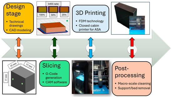
Figure 1.
Main process flow of the FDM efforts.
To measure the surface roughness results, a surface profilometer setup (Mahr MarSurf PS1 model; Göttingen, Germany) was used, and Ra results were adopted in the comparisons. Measurements were carried out at room temperature. When each pass was completed, the surface was cleaned and re-measured with the contact profilometer to obtain the corresponding roughness. Five measurements for workpiece surface roughness were carried out and averaged for each pass. The cutting length (Lc) was chosen as 0.8 mm and the sampling length (Lt) as 4.8 mm for the measurement of the surface roughness values. Figure 2 demonstrates the measuring details and data collection strategy for both surface roughness and hardness evaluations.
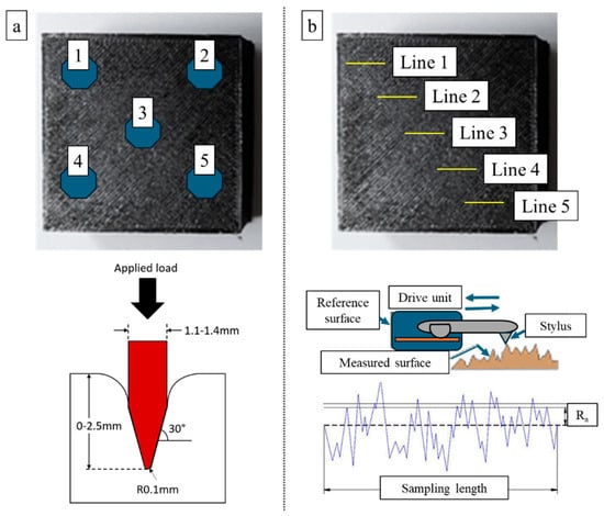
Figure 2.
Measurement points in hardness (a) and surface roughness (b) evaluations.
In the setup shown in Figure 3, the outer glass chamber was sealed with a steel lid to block the liquid and gas leakage through mechanical montage. A metallic block was placed at the center of the bottom steel lid to hinder direct contact between the liquid acetone and the target ASA samples. Thanks to its rapid delivery from the domestic suppliers, cost-effectiveness, and suitable surface interaction features, acetone was selected in this work even though dimethylformamide (DMF) and dichloromethane were also tried for acrylonitrile-based polymers. The outer glass chamber was covered with an acetone-doped towel, and an extra interlayer was created to feed the acetone gas environment with additional vapor, thereby providing better gas uniformity in the chamber. The vapor chamber volume was 400 cm3, and a total of 30 mL of acetone was used in the chamber. Also, all treatments were conducted at room temperature, and the macro-scale shape transformations were monitored with glass outer frames. At the bottom side of the chamber, an acetone pool was formed to compound the upward vapor delivery. Following the installation of the vaporizing treatment setup, four different application durations were appointed as 15, 45, 90, and 120 min. For each test, a new vapor environment was built in order to attain identical conditions. Moreover, together with vaporizing, all input variables and their levels in this work can be monitored in Table 2.
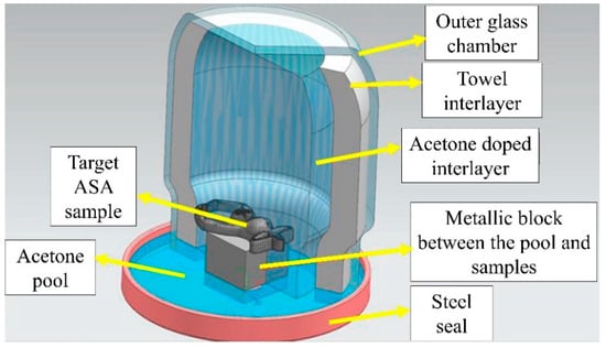
Figure 3.
Schematic view of the vaporizing environment and equipment.

Table 2.
Input variables and their levels.
2.2. Machine Learning (ML) and Deep Learning (DL) Details
This study applied a broad set of machine learning (ML) and deep learning (DL) models to predict hardness and surface roughness from additive manufacturing process data, focusing on algorithms with distinct strengths for handling nonlinear multi-target problems. Gradient boosting (GB) [34] and its optimized variant XGBoost [35] leveraged sequential error correction and regularization to efficiently capture complex parameter–property relationships. Ensemble tree methods such as Random Forest (RF) [36], Extra Trees (ETs) [37], and bagging [38] enhanced robustness to noise through randomized feature and sample selection, while stacking [39] integrated multiple base models to exploit complementary predictive capabilities. AdaBoost [40] builds an ensemble of weak learners sequentially, where each new model places greater weight on previously misclassified samples. This iterative reweighting strategy often improves predictive accuracy compared to a single base learner. However, because AdaBoost continues to emphasize all misclassified points, it can overfit when the dataset contains noisy or mislabeled samples, leading to reduced generalization performance.
DL approaches were included for their ability to learn representations from raw or minimally processed inputs. Multi-Layer Perceptrons [41] (MLPs) modeled general nonlinear relationships, while one-dimensional convolutional neural networks [42] (1D-CNNs) identified local dependencies in sequential parameter data and two-dimensional convolutional neural networks (2D-CNNs) processed structured grid-like input formats. Recurrent neural networks (RNNs) and Long Short-Term Memory [43] (LSTM) were incorporated to capture temporal dependencies across sequential layers, with LSTMs improving long-term memory retention. Traditional regression and proximity-based methods provided interpretable baselines. Support vector regressor [44] (SVR) demonstrated strong performance in nonlinear regression tasks, achieving the best performance when combined with 1D-CNN feature extraction. Decision Trees [45] (DTs) offered interpretability but were less robust alone, while K-Nearest Neighbor [46] (KNN) exploited parameter similarity for predictions. Ridge [47] and Bayesian Ridge [48] regression added regularization and uncertainty estimation, and linear regression [49] (LR) served as a simple reference point.
From a technical perspective, the chosen algorithms operate on distinct learning principles that influence their suitability for nonlinear multi-target regression tasks. GB and XGBoost construct additive models in a forward stage-wise fashion, where each successive tree is trained to minimize the residual errors of its predecessors, incorporating shrinkage (learning rate) and regularization terms to improve generalization. RF and ET utilize bootstrap aggregation (bagging) to train multiple DTs on random feature subsets, with RF using optimal splits and ETs using randomized split points to increase diversity among trees. Bagging reduces variance by averaging predictions from multiple base learners, while stacking integrates heterogeneous models through a meta-learner that is trained on their outputs. AdaBoost adapts to model weaknesses by iteratively reweighting misclassified or poorly predicted samples, focusing the learning process on more complicated cases.
DL models, in contrast, learn hierarchical feature abstractions through multiple layers of nonlinear transformations. MLPs consist of fully connected layers that map input features to outputs via learned weight matrices and activation functions, enabling flexible nonlinear modeling. CNNs apply learnable convolutional kernels to detect local patterns; in 1D-CNNs, these patterns occur along a single dimension (e.g., sequential process parameters), whereas in 2D-CNNs they operate across two-dimensional grids (e.g., spatially organized data). RNNs capture temporal or sequential dependencies by maintaining hidden states across time steps, with LSTMs enhancing this capability via gated mechanisms that regulate information flow and retain long-term dependencies. SVR maps inputs into high-dimensional feature spaces using kernel functions and constructs an optimal regression hyperplane within a defined margin of tolerance (), making it well-suited for smooth nonlinear predictions. KNN bases its predictions on the average (or weighted average) of the nearest neighbors in feature space, while Ridge and Bayesian Ridge regression introduce -norm penalties to the loss function to control coefficient magnitudes, with Bayesian Ridge additionally modeling the regression problem probabilistically to account for uncertainty. LR, as the simplest baseline, assumes a purely linear relationship between inputs and targets without regularization, serving as a reference for performance gains achieved by more complex models.
In this study, a key enhancement was the integration of 1D-CNN-based feature extraction before regression, which reduced data dimensionality and transformed high-variance manufacturing parameters into compact discriminative representations. This hybrid approach substantially improved anticipation accuracy and generalization, thereby enabling simultaneous estimation of hardness and roughness without additional sensing hardware specific to this study.
2.3. Performance Metrics
In the present study, the predictive capabilities of the developed ML and DL models were systematically assessed using three complementary statistical metrics: the coefficient of determination (), mean squared error (MSE), and root mean squared error (RMSE). These metrics were selected to provide a comprehensive evaluation of model performance in terms of accuracy, error magnitude, and generalization capability for both hardness and surface roughness prediction. The , defined in Equation (1), quantifies the proportion of variance in the target variable that is explained by the model.
Here, denotes the actual target value, the predicted value, the mean of the actual values, and the total number of samples. While provides an overall measure of quality of fit, it does not reflect the absolute magnitude of prediction errors. To address this, the MSE was computed, as given in Equation (2):
MSE penalizes larger deviations more severely, making it highly sensitive to significant prediction errors caused by variations in process parameters or measurement noise. To express the error in the same physical units as the measured properties, the RMSE was employed, as shown in Equation (3):
RMSE allows for a direct comparison of prediction errors to tolerances that are acceptable in industrial applications. This provides a practical perspective on the suitability of models for deployment in manufacturing environments. All performance metrics were calculated using a five-fold cross-validation procedure. The dataset was randomly partitioned into five equal subsets. In each iteration, four subsets were used for training, and one subset was used for testing. The final performance scores represent the average of all folds, which minimizes bias due to data partitioning and ensures a robust evaluation of the entire dataset.
3. Results and Discussion
3.1. Experimental Analyses
Figure 4 demonstrates the Shore D hardness scores of the vapor-treated ASA samples depending on the shifting infill rates and layer thicknesses. From the outcomes, the highest average hardness value of 75.6 Shore D (with a standard deviation (SD) of 2.08) was detected for the 100% filled samples subjected to 45 min vaporizing treatment, whereas the lowest average hardness of 36.6 Shore D (SD: 1.15) belonged to the 20% filled samples subjected to 120 min vaporizing. Up to 45 min, a positive effect of the acetone was observed due to its polarized molecular structure, which triggers the reaction rate and improves bond structures [50]. However, with a rising vapor treatment duration, chain relaxation mechanisms emerge, and localized fusion rates gain non-uniform characteristics. Based on the complete dataset, no consistent increasing or decreasing trend was observed between the parameter sets and the measured hardness values. At this point, it can be observed that there is a turning point for a 45-min vaporizing time, and the measured hardness values start to drop after this time due to the ascending softening effect of gas treatment. Initially, the ASA samples have several peak and valley structures on their surfaces that may cause relatively large cavities on the test surfaces. However, after up to 45 min of vaporizing time, those kinds of cavities become smaller, and surface uniformity increases. This phenomenon is the probable reason for the hardness improvement in 45 min of vaporizing. On the other hand, rising layer thickness levels triggered higher hardness results for all the samples. This case can be explained by the escalating stacking layer amount due to its strong stacking ability against the converse loading forces. As for the infill rate, it can be proposed that, as the load-carrying polymer strut volume increases, the average hardness results increase to the peak levels. However, since vaporizing is effective solely on the limited volume of the part surface, the influence of the infill rate cannot be qualified as linear.
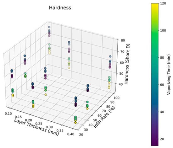
Figure 4.
Hardness results depending on the layer thickness, infill rates, and vaporizing time.
Figure 5 shows the roughness values of the tested ASA samples according to altering the infill rate, layer thickness, and vaporizing time. The results show that there was a turning point in the 90-min vaporizing time, and this duration is the best option for the most successful surface quality. For the 50% filled samples, the lowest average roughness of 0.36 µm (SD: 0.08) was recorded, and the layer thickness was 0.1 mm. The highest average roughness of 8.08 µm (SD: 0.1) was detected for the sample with a 0.4 mm layer thickness and 45 min of vaporizing. This observation can be attributed to the optimized fusion of interlayers modified by consistent exposure to acetone vapor, thereby stimulating robust cohesion between the printing layers [51]. Also, the interlayer diffusion rate reaches a balanced level after 90 min of vaporization, localized corrugated sections decrease, and surface tops and valleys are minimized with steady-state fusion. With rising vaporizing time, the smoothing capacity of the acetone gas increases, and the diffusion ability on the sample surfaces enhances the atomic activity in the vicinity of rough cavities. Nevertheless, with more vaporizing time, excess softening effects were seen, and surface flows with unwanted waviness were present on the ASA parts. As the vaporizing duration reached 120 min, although the average roughness was still lower than the initial measurements, the highest-quality surfaces were obtained in the optimum conditions at 90 min. Additionally, lower layer thickness levels were advantageous for better surface view because of the closely packed production layers, causing smaller printing gaps to be closed by the gas treatment.
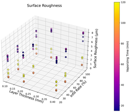
Figure 5.
Surface roughness results depending on the layer thickness, infill rates, and vaporizing time.
3.2. Machine Learning and Deep Learning Evaluations
The experiments were conducted on a high-performance desktop computer with a processor (Intel Core i9-13900K, Intel, Santa Clara, CA, USA) and dedicated GPU (NVIDIA RTX 4080, Nvidia, Santa Clara, CA, USA). All models were implemented in the Python (3.12) programming environment. ML models were developed using the scikit-learn library, and CNN-based models were implemented using the TensorFlow framework.
The dataset consisted of 108 experimental observations according to average values and is shared in Table 3. Three independent input variables were used: layer thickness, vaporizing time, and infill rate. The prediction targets were two continuous output variables: hardness and surface roughness.

Table 3.
Original dataset.
Three independent variables, layer thickness (mm), vaporizing time (min), and infill rate (%), were selected based on their known influence on the mechanical and surface characteristics of additively manufactured materials. The dependent variables were defined as hardness (Shore D) and surface roughness (µm), representing key performance indicators of the fabricated parts. The selection of these parameters was initially guided by process physics and previous studies, which report that layer thickness, post-processing duration, and infill density significantly affect material compaction and surface morphology. Correlation analyses were performed using the Pearson method to statistically validate the variable selection. As illustrated in Figure 6, the results revealed strong negative correlations between vaporizing time and both hardness (r = −0.72) and surface roughness (r = −0.80), indicating that prolonged vaporization decreases hardness and improves surface quality. Moderate relationships were also found between layer thickness and hardness (r = −0.40), and between infill rate and hardness (r = +0.35). Furthermore, the low intercorrelation among the input variables (|r| < 0.1) confirmed the absence of multicollinearity, ensuring that each input contributes independent information to the model. These findings collectively validate that the chosen independent and dependent variables are both physically meaningful and statistically justified for the regression framework.
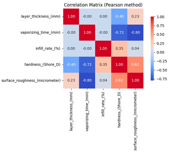
Figure 6.
Correlation matrix of the dataset.
To evaluate the model performance, the dataset was partitioned into training and testing subsets using a five-fold cross-validation strategy. In each fold, 86 samples (approximately 80%) were used for training the model, and the remaining 22 samples (approximately 20%) were reserved for testing. This ensured that each data point was included in both the training and testing phases across different folds, thereby improving the reliability and generalizability of the evaluation results.
Both the ML- and CNN-based models had a three-input, two-output architecture. In this configuration, the three process parameters (layer thickness, steaming time, and occupancy rate) were simultaneously provided as inputs to the model. These features were processed in parallel or joint feature-extraction pathways, enabling the models to capture the relationships and potential interactions between the parameters. The models then produced two separate predictions, one corresponding to hardness and the other to surface roughness, enabling simultaneous multi-target regression. Table 4 presents the detailed configurations, hyperparameters, and architectural parameters of the models used in this study.

Table 4.
Structure and parameters of the ML and DL models.
In addition to the main experimental setup, 1D-CNNs were used to extract features. A total of 32 representative features were extracted from the three input parameters, resulting in a feature map of size 32. This feature map was then used as input for the regression models. Incorporating the 1D-CNN feature extraction stage enabled the models to capture local patterns and parameter-specific variations present in the data. This approach allowed the regression models to focus on these localized features during training and testing, enhancing their ability to model complex relationships between process parameters and target variables. Table 5 provides the detailed architecture and parameter configurations of the feature extraction model and regression heads.

Table 5.
Structure and parameters of the feature extraction and regression heads.
The experimental study was designed to yield comprehensive and wide-ranging results by employing a diverse set of models, enabling a more thorough evaluation of predictive performance. Furthermore, combining ML and DL approaches allowed the study to leverage the strengths of both paradigms. This integration enhanced the robustness and capability of the modeling framework, improving its ability to capture linear and nonlinear relationships within the data and increasing the effectiveness and reliability of the results.
Table 6 summarizes the predictive performance of all the tested models for hardness and surface roughness, as determined by 5-fold cross-validation. The top-performing group consisted of CNN-based feature extraction combined with ensemble regressors. The best models were feature extraction with SVR (average MSE = 2.0941; average = 0.9614) and GB (average MSE = 2.2007; average = 0.958). Standalone DL models, such as 1D-CNN and 2D-CNN, achieved competitive accuracy. Notably, 1D-CNN slightly outperformed 2D-CNN, suggesting that one-dimensional convolutions are more effective at capturing structured relationships among the three process parameters. Traditional ensemble methods, including RF, bagging, and XGBoost, formed the second tier of performance, demonstrating robust, although slightly lower, accuracy. Purely linear models, such as Ridge, Bayesian Ridge, and linear regression, demonstrated poor predictive performance because they assume a strictly linear relationship between the input parameters and target variables. In this study, however, the relationships between process parameters (layer thickness, steaming time, and occupancy rate) and output properties (hardness and surface roughness) are inherently nonlinear and influenced by complex interactions. Linear models are unable to capture these dependencies, which leads to underfitting and considerably reduced accuracy, with average R2 values around 0.69.

Table 6.
Performance results of the models.
By contrast, combining Ridge regression with CNN-based feature extraction (feature extraction with Ridge) markedly improved performance (avg R2 = 0.9556 compared with 0.6942 for standard Ridge). This enhancement arises because the 1D-CNN feature extractor transforms the three raw inputs into thirty-two higher-level features that encode nonlinear relationships and localized patterns. Projecting the data into this enriched feature space reshapes the problem so that the relationships between features and outputs become closer to linear. In this transformed domain, Ridge regression can operate effectively, applying regularization to prevent overfitting while exploiting the structure already embedded in the extracted features. The observed performance gain, therefore, highlights that the limitation of Ridge lies not in its optimization mechanism but in the inadequacy of raw inputs. Once the inputs are expressed through CNN-derived representations, even a simple linear model can achieve predictive accuracy comparable to more sophisticated algorithms. The fold-level performance of the top five models is provided in Table 7.

Table 7.
Five-fold results of the top three models and the worst model.
A fold-level analysis of the top five models (see Table 7) confirmed that they all maintained values above 0.94 across folds, indicating consistent predictive capability. Feature extraction with SVR displayed slightly higher variability in MSE between folds, likely due to changes in target value distributions. In contrast, 1D-CNN and GB exhibited strong stability in certain folds with notably low errors. Figure 7 visually supports these findings, showing that the predicted values closely track the actual measurements across all folds with minimal deviation.
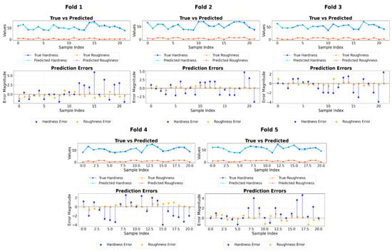
Figure 7.
Fold-by-fold prediction performance of the feature extraction with the SVR model.
Figure 8, Figure 9 and Figure 10 show the five-fold regression results of the feature extraction with SVR, GB, and RNN models for predicting hardness and surface roughness. In all cases, the predicted values align closely with the true values along the 1:1 reference line, confirming strong predictive accuracy. The feature extraction with the SVR model achieved the most consistent performance, with values ranging from 0.95 to 0.97, demonstrating its ability to generalize effectively across data partitions. Gradient boosting also produced robust results, closely tracking the true values across folds, although slight variability in prediction error indicates some sensitivity to the composition of training and testing subsets. The RNN model maintained high predictive accuracy, with values consistently above 0.94, but exhibited marginally greater dispersion around the reference line compared to the other two models.
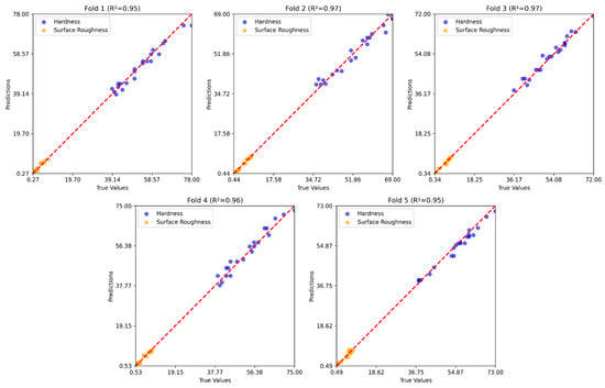
Figure 8.
Five-fold regression results of the feature extraction with the SVR model.
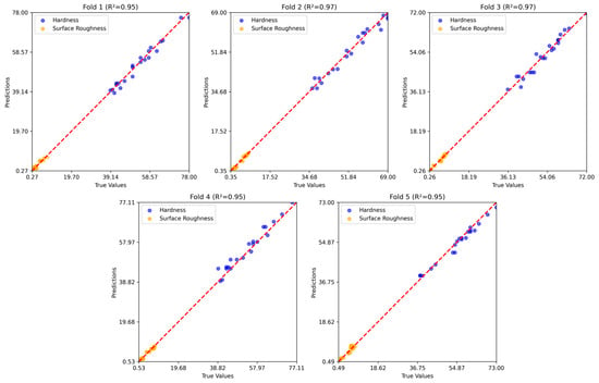
Figure 9.
Five-fold regression results of the GB model.
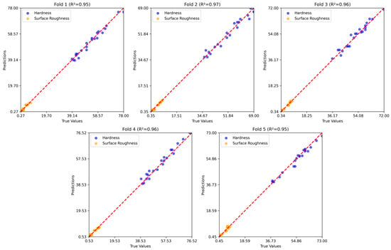
Figure 10.
Five-fold regression results of the RNN model.
To assess dataset adequacy and validate model generalization given the limited sample size (108 observations), learning curves were generated for the superior CNN–SVR model using five-fold cross-validation, as illustrated in Figure 11. Each subplot depicts the evolution of training and validation mean squared error (MSE) as a function of increasing training set size. The learning dynamics reveal a characteristic pattern across all folds: both training and validation curves exhibit rapid error reduction during the initial training phase, subsequently achieving smooth convergence toward lower MSE values. The close correspondence between training and validation trajectories throughout the learning process provides compelling evidence of effective generalization without overfitting. Notably, the absence of divergence between these curves demonstrates that the available dataset contains sufficient informational content to enable the CNN–SVR model to establish stable and representative mappings between process parameters and material properties. Furthermore, the convergence plateau observed beyond approximately 40–50 training samples indicates that the model approaches its optimal learning capacity within the limitations of the current dataset, suggesting that substantial data augmentation would yield only incremental performance gains.
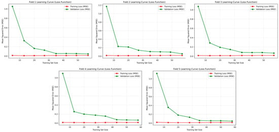
Figure 11.
Learning curves of the best-performing CNN–SVR model (training and validation losses) across five folds of cross-validation.
To provide complementary insights into model learning behavior, Figure 12 presents the coefficient of determination (R2) evolution for the CNN–SVR model across all cross-validation folds. Each subplot illustrates the progressive development of training and validation R2 scores with increasing sample size, offering additional perspective on generalization capability. The learning curves consistently demonstrate an upward trajectory across all folds, with validation R2 values steadily converging toward their training counterparts as data availability increases. This convergence pattern substantiates effective learning of the underlying input–output relationships without manifestations of underfitting or overfitting phenomena. The stabilization of both curves at elevated R2 levels (consistently exceeding 0.9) across all validation folds confirms robust predictive performance and reliable generalization despite dataset size limitations. These findings collectively validate that the CNN–SVR architecture successfully captures the complex nonlinear interdependencies among process parameters (layer thickness, infill rate, and vaporizing time), thereby enabling precise simultaneous prediction of surface roughness and hardness in ASA-based FDM components.
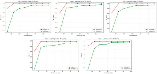
Figure 12.
Learning curves of the best-performing CNN–SVR model (R2 score) across five folds of cross-validation.
4. Discussion
ML and DL techniques have attracted considerable attention due to their ability to predict mechanical and surface properties in additive manufacturing processes. While many studies have focused on individual properties, such as hardness or surface roughness, these studies collectively demonstrate the potential of advanced algorithms to capture complex nonlinear relationships between manufacturing parameters and material performance. In this context, ensemble methods, as well as various neural network architectures, have repeatedly emerged as leading approaches. A summary of the studies conducted in this field to date is presented in Table 8.

Table 8.
Comparative summary of current research and related studies on predicting hardness and surface roughness in additive manufacturing.
For instance, Veeman et al. (2023) [54] obtained an value of 0.9136 for ABS component hardness prediction using RF, and Mahmoud et al. (2024) [56] reported an of 0.995 for PC parts using the same model. Similarly, Badogu et al. (2024) [55] obtained an of 0.955 for PLA hardness prediction using ensemble learning, which reinforces RF’s strong generalization capability across polymer-based additive manufacturing applications. Similar trends have been observed in research on surface roughness prediction, although the approaches often differ in feature sources and computational strategies. Tzotzis et al. (2025) [63] achieved a minimum mean absolute percentage error (MAPE) of 1.51% for carbon fiber-reinforced polymer (CFRP) machining by integrating vibration-derived features into artificial neural network (ANN) models. Wardhani et al. (2024) [57] employed hybrid regression techniques and reported RMSE values between 3.21 and 3.65 for surface roughness estimation. In the field of metal additive manufacturing, Panico et al. (2025) [61] applied CNN-based models to predict the mechanical properties of laser powder bed fusion, achieving an of approximately 0.94. Meanwhile, Mulugumdam et al. (2025) [59] employed XGBoost to model a single quality metric in fused deposition modeling (FDM), achieving an MSE of 0.799. While these studies demonstrate the feasibility of achieving high predictive accuracy, most prior efforts are limited to single-property modeling or depend on auxiliary sensing systems. Although these systems are effective, they increase the complexity and cost of implementation.
Unlike previous studies with a single-target scope, the present study develops a multi-target regression framework that can predict hardness and surface roughness simultaneously from process parameter data alone. The proposed model, which combines one-dimensional CNN-based feature extraction with SVR, achieved an average MSE of 2.0941 and an of 0.9614 across five-fold cross-validation. These results surpass the performance reported by Veeman et al. (2023) [54] by approximately 5.2% in and marginally exceed the accuracy of Badogu et al. (2024) [55] despite addressing a more complex prediction problem. Additionally, the framework matches Tzotzis et al.’s (2025) [63] performance in surface roughness prediction without requiring vibration-sensing hardware, thus simplifying its integration into industrial workflows. Reducing RMSE to approximately 1.45 significantly improves upon the surface roughness results reported by Wardhani et al. (2024) [57].
The superior performance of the proposed CNN–SVR hybrid can be attributed to its ability to combine the nonlinear feature extraction capacity of convolutional neural networks with the generalization stability of support vector regression. The CNN layer captures complex localized relationships between layer thickness, infill rate, and vaporizing time—relationships that directly reflect the physical interactions affecting surface finish and hardness in FDM. The SVR component then operates on these high-level features within a compact and less redundant representation space, resulting in enhanced regression accuracy and reduced overfitting.
Several factors contribute to the overall strength of the proposed methodology. The framework demonstrates versatility by effectively integrating both machine learning and deep learning paradigms, allowing the advantages of each to be leveraged in a complementary manner. It has been comprehensively benchmarked against a broad range of algorithms, ensuring a rigorous and balanced assessment of its relative performance. Moreover, the proposed model achieves high predictive accuracy without relying on costly or complex measurement systems, making it particularly suitable for rapid, low-cost, and multi-criteria quality evaluation in manufacturing environments. Despite these strengths, certain limitations remain. Although the manually designed feature extraction stage proved to be effective, it could benefit from automated optimization or dimensionality reduction techniques to further enhance adaptability and scalability. In addition, while the dataset used in this study was sufficient for the intended analysis, it was restricted to a single material type and a relatively narrow range of process parameters. Expanding the dataset to include multiple materials, part geometries, and processing conditions would likely improve the model’s generalization and robustness. Unlike many existing models that depend on extensive sensing data, the proposed framework achieves reliable predictive performance using only process parameters and post-processing conditions, underscoring its practicality for low-cost real-time quality prediction in industrial additive manufacturing applications.
Future work could further enhance prediction accuracy by integrating the representational learning capabilities of CNNs with the stability of ensemble methods in hybrid architectures. Incorporating metaheuristic optimization algorithms, such as genetic algorithms or particle swarm optimization, may improve hyperparameter tuning and model efficiency. Furthermore, using explainable AI tools, such as SHAPs or LIMEs, would provide transparency in model decision-making and yield more profound insights into process–property relationships. This would ultimately support more effective process optimization in industrial additive manufacturing.
5. Conclusions
This study focused on applying ML and DL techniques to simultaneously predict hardness and surface roughness in additively manufactured ASA components. The following key conclusions can be drawn from the outcomes of this study:
- The proposed ML–DL framework, which integrates 1D-CNN feature extraction with SVR, was highly effective in modeling the complex nonlinear relationships between process parameters and output properties.
- This approach successfully predicted two critical quality indicators, hardness and surface roughness, simultaneously, eliminating the need for separate models and additional sensing hardware.
- Among all the tested algorithms, the 1D-CNN model with SVR had the best overall performance, with an average R2 of 0.9614 and an MSE of 2.0941 across five-fold cross-validation. This model outperformed or matched the results of the leading single-target studies in the literature.
- The model demonstrated strong generalization capability, maintaining high predictive accuracy across all folds. This indicates robustness for industrial applications, where process variability is common.
- As the infill rate and layer thickness increase, the measured hardness values of the ASA parts gain an upward tendency, but this case is not valid for vaporizing time, and it should be optimized for target hardness levels.
- There is no direct increasing/decreasing relationship between surface roughness values and vaporizing time, so the best surface quality can be obtained with intermediate levels of acetone gas treatment duration.
Overall, this study bridges the gap between single-target research approaches and practical multi-target industrial solutions by demonstrating that CNN-enhanced ML models can accurately, reliably, and cost-effectively predict critical quality metrics in additive manufacturing. The proposed framework advances predictive modeling and offers a scalable real-world tool for accelerating process optimization, improving product consistency, and reducing manufacturing costs in high-performance engineering applications.
Supplementary Materials
The following supporting information can be downloaded at https://www.mdpi.com/article/10.3390/polym17212881/s1, File S1: Analysis of ISO 52900.
Author Contributions
Conceptualization, Ç.B., F.D., İ.G., B.Y., R.Ş. and A.E.; methodology, Ç.B., F.D. and İ.G.; software, İ.G. and F.D.; validation, İ.G. and F.D.; investigation, Ç.B., F.D., İ.G., B.Y., R.Ş. and A.E.; writing—original draft preparation, Ç.B., B.Y., İ.G., F.D. and A.E.; writing—review and editing, İ.G., F.D., A.E. and R.Ş.; visualization, İ.G., F.D. and R.Ş. All authors have read and agreed to the published version of the manuscript.
Funding
The authors received no specific funding for this work.
Institutional Review Board Statement
Not applicable.
Data Availability Statement
The data that support the findings of this study are available on request from the corresponding author. Additionally, the source code used for model development, training, and performance evaluation is openly available from the accompanying GitHub repository: https://github.com/FurkancanDemircan/ASA-Hardness-Roughness-MLDL (accessed day 18 October 2025).
Conflicts of Interest
The authors declare no conflicts of interest.
References
- Meng, M.; Wang, J.; Huang, H.; Liu, X.; Zhang, J.; Li, Z. 3D Printing Metal Implants in Orthopedic Surgery: Methods, Applications and Future Prospects. J. Orthop. Translat. 2023, 42, 94–112. [Google Scholar] [CrossRef]
- Lo Russo, L.; Guida, L.; Mariani, P.; Ronsivalle, V.; Gallo, C.; Cicciù, M.; Laino, L. Effect of Fabrication Technology on the Accuracy of Surgical Guides for Dental-Implant Surgery. Bioengineering 2023, 10, 875. [Google Scholar] [CrossRef]
- Bolat, Ç.; Salmaz, S. An Investigation on the Wear Properties of the Photocurable Components Produced by Additive Manufacturing for Dentistry Applications: Combined Influences of UV Exposure Time, Building Direction, and Sliding Loads. Polym. Eng. Sci. 2024, 64, 5940–5958. [Google Scholar] [CrossRef]
- Mohanavel, V.; Ashraff Ali, K.S.; Ranganathan, K.; Allen Jeffrey, J.; Ravikumar, M.M.; Rajkumar, S. The Roles and Applications of Additive Manufacturing in the Aerospace and Automobile Sector. Mater. Today Proc. 2021, 47, 405–409. [Google Scholar] [CrossRef]
- Radhika, C.; Shanmugam, R.; Ramoni, M.; Gnanavel, B.K. A Review on Additive Manufacturing for Aerospace Application. Mater. Res. Express 2024, 11, 022001. [Google Scholar] [CrossRef]
- Ko, C.-H. Constraints and Limitations of Concrete 3D Printing in Architecture. J. Eng. Des. Technol. 2022, 20, 1334–1348. [Google Scholar] [CrossRef]
- Xiao, Y.-Q.; Kan, C.-W. Review on Development and Application of 3D-Printing Technology in Textile and Fashion Design. Coatings 2022, 12, 267. [Google Scholar] [CrossRef]
- Bolat, Ç.; Yıldırım, E. A Comparative Effort on the Influence of Liquid Treatment Media Type, Fiber Addition, and Deformation Load on the Wear Performance of Additively Manufactured Polyamide 6 and Acrylonitrile Butadiene Styrene Composites. Polym. Compos. 2025, 46, 10619–10635. [Google Scholar] [CrossRef]
- Izdebska-Podsiadły, J. Classification of 3D Printing Methods. In Polymers for 3D Printing; William Andrew Publishing: Norwich, NY, USA, 2022; Volume 1, pp. 23–34. [Google Scholar]
- Mohamed, O.A.; Masood, S.H.; Bhowmik, J.L. A Parametric Investigation of the Friction Performance of PC-ABS Parts Processed by FDM Additive Manufacturing Process. Polym. Adv. Technol. 2017, 28, 1911–1918. [Google Scholar] [CrossRef]
- Caussin, E.; Moussally, C.; Le Goff, S.; Fasham, T.; Troizier-Cheyne, M.; Tapie, L.; Dursun, E.; Attal, J.-P.; François, P. Vat Photopolymerization 3D Printing in Dentistry: A Comprehensive Review of Actual Popular Technologies. Materials 2024, 17, 950. [Google Scholar] [CrossRef]
- Han, M.; Kaşıkcıoğlu, S.; Ergene, B.; Atlıhan, G.; Bolat, Ç. An Experimental Investigation on the Mechanical and Wear Responses of Lightweight AlSi10Mg Components Produced by Selective Laser Melting: Effects of Building Direction and Test Force. Sci. Sinter. 2025, 57, 87–101. [Google Scholar] [CrossRef]
- Reyes-Luna, J.F.; Chang, S.; Tuck, C.J.; Ashcroft, I.A. Material Jetting High Quality Components via an Inverse Problem Framework. Addit. Manuf. 2023, 73, 103667. [Google Scholar] [CrossRef]
- Zhang, K.; Zhang, W.; Brune, R.; Herderick, E.; Zhang, X.; Cornell, J.; Forsmark, J. Numerical Simulation and Experimental Measurement of Pressureless Sintering of Stainless Steel Part Printed by Binder Jetting Additive Manufacturing. Addit. Manuf. 2021, 47, 102330. [Google Scholar] [CrossRef]
- Alammar, A.; Kois, J.C.; Revilla-León, M.; Att, W. Additive Manufacturing Technologies: Current Status and Future Perspectives. J. Prosthodont. 2022, 31, 4–12. [Google Scholar] [CrossRef]
- Riensche, A.; Severson, J.; Yavari, R.; Piercy, N.L.; Cole, K.D.; Rao, P. Thermal Modeling of Directed Energy Deposition Additive Manufacturing Using Graph Theory. Rapid Prototyp. J. 2023, 29, 324–343. [Google Scholar] [CrossRef]
- Bolat, Ç.; Ergene, B. Wear Performance of Short Fiber Added Polyamide Composites Produced by Additive Manufacturing: Combined Impacts of Secondary Heat Treatment, Reinforcement Type, and Test Force. Polym. Compos. 2024, 45, 6885–6900. [Google Scholar] [CrossRef]
- Mendenhall, R.; Eslami, B. Experimental Investigation on Effect of Temperature on FDM 3D Printing Polymers: ABS, PETG, and PLA. Appl. Sci. 2023, 13, 11503. [Google Scholar] [CrossRef]
- Bolat, Ç.; Aslan, M.T.; Çebi, A.; Gene, T.E.; Ispartalı, H. A Comprehensive Analysis of the Influence of Adhesive Types and Layer Stacking Sequence on Tensile and Impact Responses of ASA/PLA Composite Sandwich Structures by Additive Manufacturing. J. Polym. Res. 2025, 32, 174. [Google Scholar] [CrossRef]
- Daly, M.; Tarfaoui, M.; Chihi, M.; Bouraoui, C. FDM Technology and the Effect of Printing Parameters on the Tensile Strength of ABS Parts. Int. J. Adv. Manuf. Technol. 2023, 126, 5307–5323. [Google Scholar] [CrossRef]
- Özen, A.; Abali, B.E.; Völlmecke, C.; Gerstel, J.; Auhl, D. Exploring the Role of Manufacturing Parameters on Microstructure and Mechanical Properties in Fused Deposition Modeling (FDM) Using PETG. Appl. Compos. Mater. 2021, 28, 1799–1828. [Google Scholar] [CrossRef]
- Desai, S.M.; Sonawane, R.Y.; More, A.P. Thermoplastic Polyurethane for Three-dimensional Printing Applications: A Review. Polym. Adv. Technol. 2023, 34, 2061–2082. [Google Scholar] [CrossRef]
- Wojnowski, W.; Marć, M.; Kalinowska, K.; Kosmela, P.; Zabiegała, B. Emission Profiles of Volatiles during 3D Printing with ABS, ASA, Nylon, and PETG Polymer Filaments. Molecules 2022, 27, 3814. [Google Scholar] [CrossRef]
- Hameed, A.Z.; Aravind Raj, S.; Kandasamy, J.; Shahzad, M.A.; Baghdadi, M.A. 3D Printing Parameter Optimization Using Taguchi Approach to Examine Acrylonitrile Styrene Acrylate (ASA) Mechanical Properties. Polymers 2022, 14, 3256. [Google Scholar] [CrossRef]
- Vidakis, N.; Petousis, M.; Michailidis, N.; Sagris, D.; David, C.; Papadakis, V.; Spyridaki, M.; Argyros, A.; Valsamos, I.; Dimitriou, E.; et al. Thermomechanical Recyclability of Acrylonitrile Styrene Acrylate (ASA) for Cyclic Economy-Driven MEX Additive Manufacturing. Clean. Eng. Technol. 2025, 25, 100925. [Google Scholar] [CrossRef]
- Tripathy, C.R.; Sharma, R.K.; Rattan, V.K. An Investigation on Mechanical Strength of Fused Filament Fabricated and Injection Molded ASA Parts. J. Micromanuf. 2025, 8, 44–59. [Google Scholar] [CrossRef]
- Rakshit, R.; Kalvettukaran, P.; Acharyya, S.K.; Panja, S.C.; Misra, D. Development of High Specific Strength Acrylonitrile Styrene Acrylate (ASA) Structure Using Fused Filament Fabrication. Prog. Addit. Manuf. 2023, 8, 1543–1553. [Google Scholar] [CrossRef]
- Raut, N.P.; Kolekar, A.B. Experimental Analysis of 3D Printed Specimens with Different Printing Parameters for Izod Impact Strength. Mater. Today Proc. 2023, 80, 156–162. [Google Scholar] [CrossRef]
- Maraş, S.; Bolat, Ç.; Çebi, A.; Ergene, B. Free Vibration Analysis of Polymer-Based Sandwich Composite Tapered Beams: Experimental and Numerical Investigation. Int. J. Struct. Stab. Dyn. 2025. [Google Scholar] [CrossRef]
- Gawali, S.K.; Jain, P.K. Effect of Natural Aging on Mechanical Properties of 3D-Printed Acrylonitrile Styrene Acrylate for Outdoor Applications. J. Mater. Eng. Perform. 2025, 34, 16430–16442. [Google Scholar] [CrossRef]
- Moreno Sánchez, D.; Hernández Saz, J.; Relinque Madroñal, J.J.; Burgos Pintos, P.; Molina Rubio, S.I.; Herrera Collado, M. Influence of Manufacturing Process in Pores, Fibre Distribution and Mechanical Properties of ASA-CF for 3D Large Format Additive Manufacturing Pieces. Rapid Prototyp. J. 2025, 31, 218–230. [Google Scholar] [CrossRef]
- Captan Prabakaran, A.; Senthil, P.; Sathies, T. Effect of Post-Processing Technique on the Mechanical, Tribological Behavior and Surface Characteristics of 3D-Printed Acrylonitrile Styrene Acrylate Parts. Surf. Rev. Lett. 2022, 29, 2250101. [Google Scholar] [CrossRef]
- Petousis, M.; Maniadi, A.; Papadakis, V.; Mountakis, N.; Argyros, A.; Efstratiadis, V.S.; David, C.; Sagris, D.; Michailidis, N.; Vidakis, N. Optimization of Nano-Silicon Nitride Content in Acrylonitrile Styrene Acrylate for Material Extrusion 3D Printing: Engineering Response Metrics. J. Mater. Eng. Perform. 2025, 34, 20505–20525. [Google Scholar] [CrossRef]
- Friedman, J.H. Greedy Function Approximation: A Gradient Boosting Machine. Ann. Stat. 2001, 29, 1189–1232. [Google Scholar] [CrossRef]
- Chen, T.; Guestrin, C. XGBoost: A Scalable Tree Boosting System. arXiv 2016, arXiv:1603.02754. [Google Scholar] [CrossRef]
- Breiman, L. Random Forests. Mach. Learn. 2001, 45, 5–32. [Google Scholar] [CrossRef]
- Geurts, P.; Ernst, D.; Wehenkel, L. Extremely Randomized Trees. Mach. Learn. 2006, 63, 3–42. [Google Scholar] [CrossRef]
- Breiman, L. Bagging Predictors. Mach. Learn. 1996, 24, 123–140. [Google Scholar] [CrossRef]
- Wolpert, D.H. Stacked Generalization. Neural Netw. 1992, 5, 241–259. [Google Scholar] [CrossRef]
- Freund, Y.; Schapire, R.E. A Decision-Theoretic Generalization of On-Line Learning and an Application to Boosting. J. Comput. Syst. Sci. 1997, 55, 119–139. [Google Scholar] [CrossRef]
- Amari, S.; Park, H.; Fukumizu, K. Adaptive Method of Realizing Natural Gradient Learning for Multilayer Perceptrons. Neural Comput. 2000, 12, 1399–1409. [Google Scholar] [CrossRef] [PubMed]
- LeCun, Y.; Bengio, Y.; Hinton, G. Deep Learning. Nature 2015, 521, 436–444. [Google Scholar] [CrossRef] [PubMed]
- Hochreiter, S.; Schmidhuber, J. Long Short-Term Memory. Neural Comput. 1997, 9, 1735–1780. [Google Scholar] [CrossRef]
- Evgeniou, T.; Pontil, M. Support Vector Machines: Theory and Applications. In Lecture Notes in Computer Science; Lecture Notes in Artificial Intelligence and Lecture Notes in Bioinformatics; Springer: Berlin/Heidelberg, Germany, 2001; Volume 2049, pp. 249–257. [Google Scholar]
- Quinlan, J.R. Induction of Decision Trees. Mach. Learn. 1986, 1, 81–106. [Google Scholar] [CrossRef]
- Cover, T.; Hart, P. Nearest Neighbor Pattern Classification. IEEE Trans. Inf. Theory 1967, 13, 21–27. [Google Scholar] [CrossRef]
- Hoerl, A.E.; Kennard, R.W. Ridge Regression: Biased Estimation for Nonorthogonal Problems. Technometrics 1970, 12, 55–67. [Google Scholar] [CrossRef]
- Hsiang, T.C. A Bayesian View on Ridge Regression. J. R. Stat. Soc. Ser. D Stat. 1975, 24, 267–268. [Google Scholar] [CrossRef]
- Stanton, J.M. Galton, Pearson, and the Peas: A Brief History of Linear Regression for Statistics Instructors. J. Stat. Educ. 2001, 9. [Google Scholar] [CrossRef]
- Demircali, A.A.; Yilmaz, D.; Yilmaz, A.; Keskin, O.; Keshavarz, M.; Uvet, H. Enhancing Mechanical Properties and Surface Quality of FDM-Printed ABS: A Comprehensive Study on Cold Acetone Vapor Treatment. Int. J. Adv. Manuf. Technol. 2024, 130, 4027–4039. [Google Scholar] [CrossRef]
- Aguilar, F.B.J.; Varela-Soriano, J.; Medina-Castro, A.; Torres-Cedillo, S.G.; Cortes-Perez, J.; Jimenez-Martinez, M. Post-Fabrication Treatment Process for ABS Printed Parts Using Acetone Vapor. Prog. Addit. Manuf. 2025, 10, 1561–1574. [Google Scholar] [CrossRef]
- Hossain, M.I.; Chowdhury, M.A.; Zahid, M.S.; Sakib-Uz-Zaman, C.; Rahaman, M.L.; Kowser, M.A. Development and Analysis of Nanoparticle Infused Plastic Products Manufactured by Machine Learning Guided 3D Printer. Polym. Test. 2022, 106, 107429. [Google Scholar] [CrossRef]
- Batu, T.; Lemu, H.G.; Shimels, H. Application of Artificial Intelligence for Surface Roughness Prediction of Additively Manufactured Components. Materials 2023, 16, 6266. [Google Scholar] [CrossRef]
- Veeman, D.; Sudharsan, S.; Surendhar, G.J.; Shanmugam, R.; Guo, L. Machine Learning Model for Predicting the Hardness of Additively Manufactured Acrylonitrile Butadiene Styrene. Mater. Today Commun. 2023, 35, 106147. [Google Scholar] [CrossRef]
- Badogu, K.; Thakur, V.; Kumar, R.; Kumar, R.; Singh, S. Acrylonitrile Butadiene Styrene-ZrO2 Composites for Roller Burnishing as Post-Processing of 3D Printed Parts: Machine Learning Modeling Using Classification and Regression Trees. J. Mater. Eng. Perform. 2024, 33, 9522–9533. [Google Scholar] [CrossRef]
- Mahmoud, A.H.; Shanmugasundar, G.; Vyavahare, S.; Kumar, R.; Cep, R.; Salunkhe, S.; Gawade, S.; Abouel Nasr, E.S. Prediction of Machine Learning-Based Hardness for the Polycarbonate Using Additive Manufacturing. Front. Mater. 2024, 11, 1410277. [Google Scholar] [CrossRef]
- Wardhani, R.; Nurhadi, H.; Guntur, H.L. Prediction of Surface Roughness and Hardness on Multi 3D Printers with Machine Learning. In Proceedings of the 2024 International Automatic Control Conference (CACS), Taiwan, China, 31 October–3 November 2024. [Google Scholar]
- Kadauw, A.A.A. Neural Network Optimization of Mechanical Properties of ABS-like Photopolymer Utilizing Stereolithography (SLA) 3D Printing. J. Manuf. Mater. Process. 2025, 9, 116. [Google Scholar] [CrossRef]
- Mulugundam, S.S.; Gugulothu, S.K.; Varshith, M. A Machine Learning Approach to Refining Surface Quality and Material Durability in Additive Manufacturing. Prog. Addit. Manuf. 2025, 10, 7779–7790. [Google Scholar] [CrossRef]
- Özkül, M.; Kuncan, F.; Ulkir, O. Predicting Mechanical Properties of FDM-Produced Parts Using Machine Learning Approaches. J. Appl. Polym. Sci. 2025, 142, e56899. [Google Scholar] [CrossRef]
- Panico, A.; Corvi, A.; Collini, L.; Sciancalepore, C. Multi Objective Optimization of FDM 3D Printing Parameters Set via Design of Experiments and Machine Learning Algorithms. Sci. Rep. 2025, 15, 16753. [Google Scholar] [CrossRef] [PubMed]
- Reddy, B.V.S.; Shaik, A.M.; Sastry, C.C.; Krishnaiah, J.; Patil, S.; Nikhare, C.P. Performance Evaluation of Machine Learning Techniques in Surface Roughness Prediction for 3D Printed Micro-Lattice Structures. J. Manuf. Process 2025, 137, 320–341. [Google Scholar] [CrossRef]
- Tzotzis, A.; Maropoulos, P.; Kyratsis, P. A Dynamic Surface Roughness Prediction System Based on Machine Learning for the 3D-Printed Carbon-Fiber-Reinforced-Polymer (CFRP) Turning. J. Intell. Manuf. 2025. [Google Scholar] [CrossRef]
Disclaimer/Publisher’s Note: The statements, opinions and data contained in all publications are solely those of the individual author(s) and contributor(s) and not of MDPI and/or the editor(s). MDPI and/or the editor(s) disclaim responsibility for any injury to people or property resulting from any ideas, methods, instructions or products referred to in the content. |
© 2025 by the authors. Licensee MDPI, Basel, Switzerland. This article is an open access article distributed under the terms and conditions of the Creative Commons Attribution (CC BY) license (https://creativecommons.org/licenses/by/4.0/).