
A Tale of Two Chains: Geometries of a Chain Model and Protein Native State Structures

 , , ,
, , ,  and
and
Abstract
1. Introduction
2. Materials and Methods
2.1. Our Protein Dataset
2.2. Numerical Simulations of a Chain of Tethered Tangent Spheres
3. General Considerations
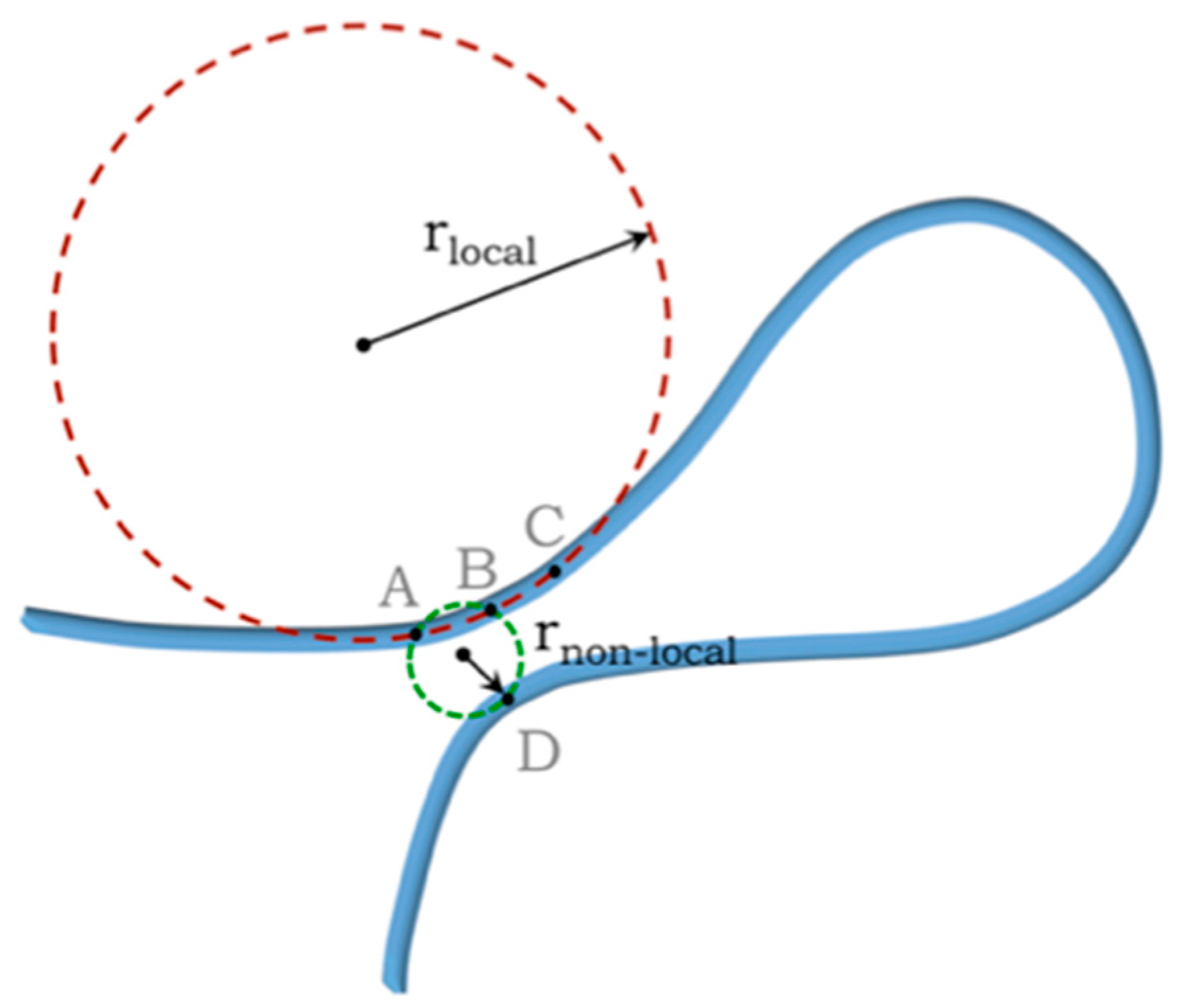
Three-Body Interactions and the Self-Avoidance of a Continuum Tube
4. Results
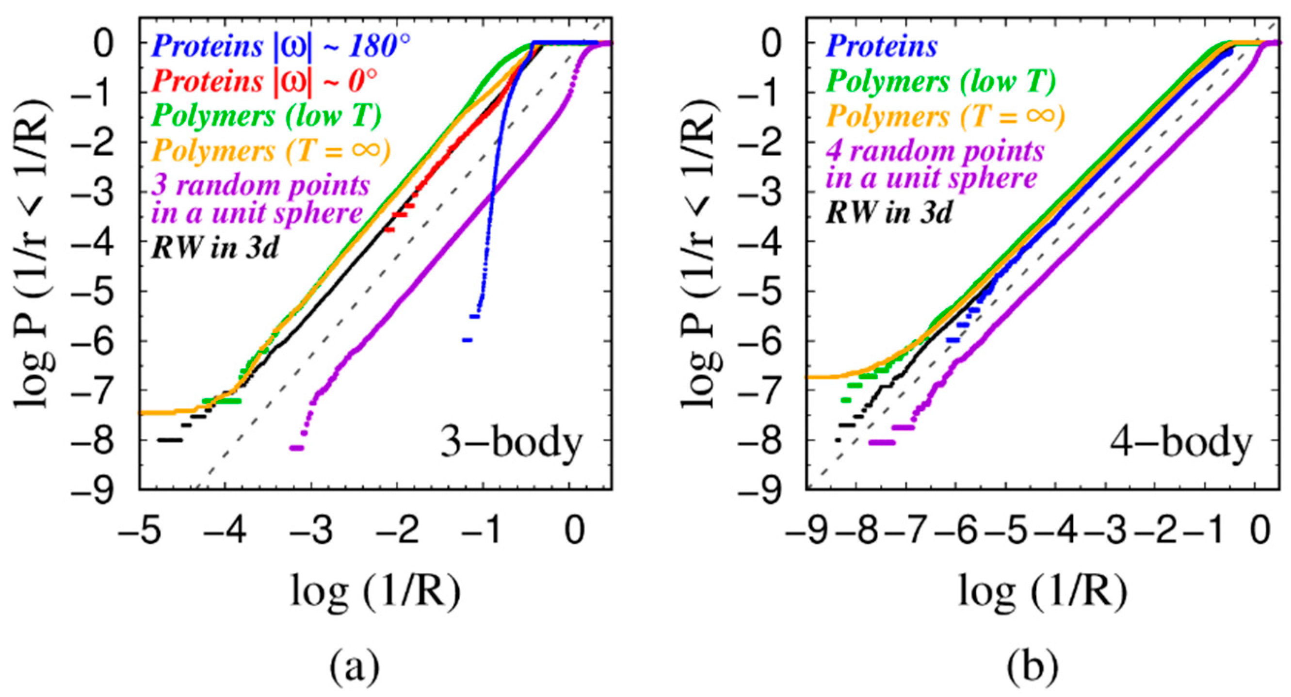
4.1. Power Law Scaling

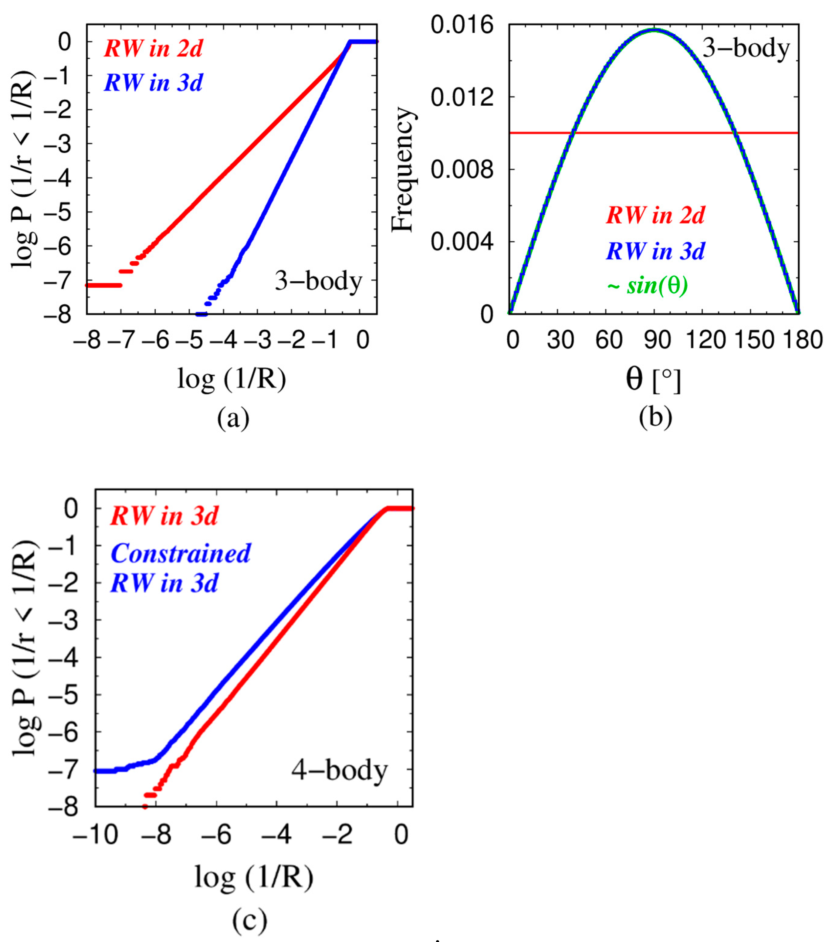
4.2. Rationalization of the Power-Law Exponent
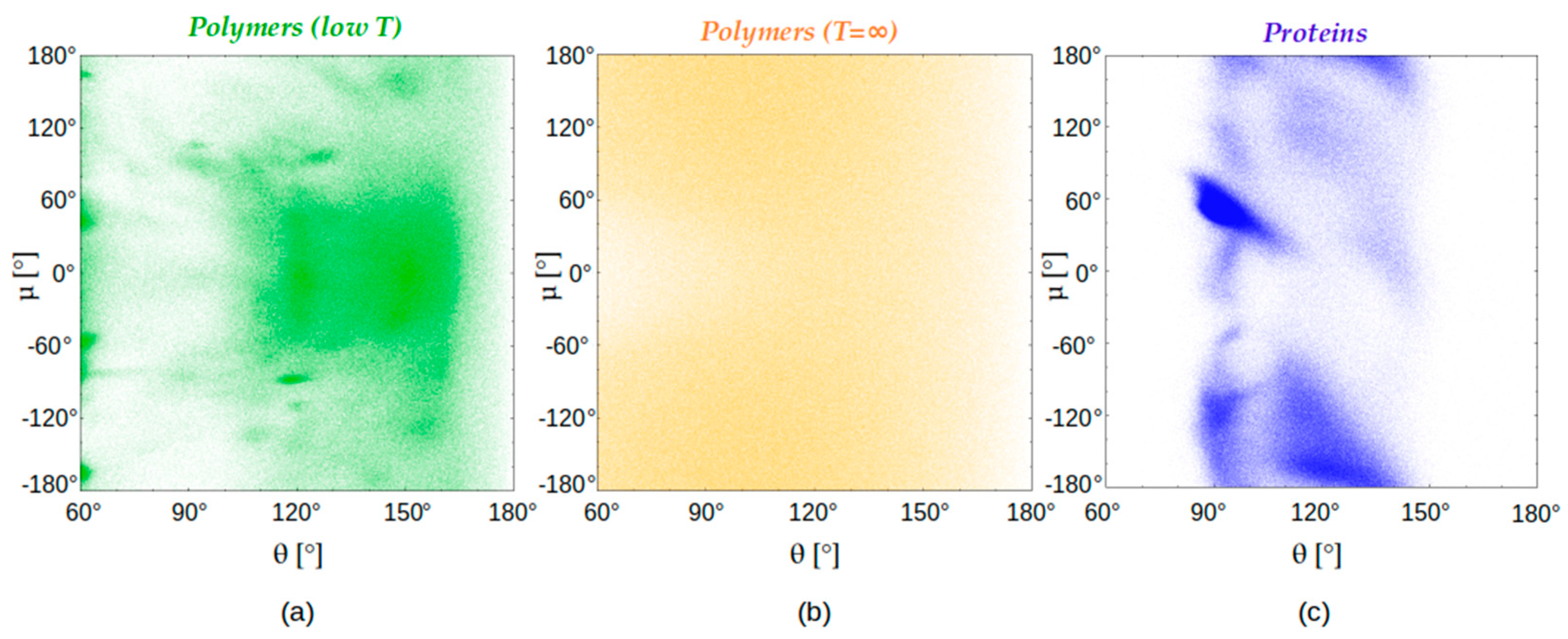
4.3. Chain Geometries
5. Discussion
Author Contributions
Funding
Institutional Review Board Statement
Data Availability Statement
Conflicts of Interest
References
- Flory, P. Statistical Mechanics of Chain Molecules; Inter-Science Publishers: New York, NY, USA, 1969. [Google Scholar]
- de Gennes, P.G. Scaling Concepts in Polymer Physics; Cornell University Press: Ithaca, NY, USA, 1979. [Google Scholar]
- Khokhlov, A.R.; Grosberg, A.Y.; Pande, V.S. Statistical Physics of Macromolecules (Polymers and Complex Materials), 4th ed.; American Institute of Physics: New York, NY, USA, 2002. [Google Scholar]
- Rubinstein, M.; Colby, R.H. Polymer Physics (Chemistry), 1st ed; Oxford University Press: London, UK, 2003. [Google Scholar]
- Kratky, O.; Porod, G. Röntgenuntersushung gelöster Fagenmoleküle. Rec. Trav. Chim. Pays Bas 1949, 68, 1106–1123. [Google Scholar] [CrossRef]
- Schellman, J.A. Flexibility of DNA. Biopolymers 1974, 13, 217–226. [Google Scholar] [CrossRef]
- Bustamante, C.; Bryant, Z.; Smith, S.B. Ten years of tension: Single-molecule DNA mechanics. Nature 2003, 421, 423–427. [Google Scholar] [CrossRef]
- Kauzmann, W. Some factors in interpretation of protein denaturation. Adv. Protein Chem. 1959, 14, 1–63. [Google Scholar] [CrossRef]
- Privalov, P.L.; Gill, S.J. Stability of protein structure and hydrophobic interaction. Adv. Protein Chem. 1988, 39, 191–234. [Google Scholar] [CrossRef]
- Dill, K.A. Dominant forces in protein folding. Biochemistry 1990, 29, 7133–7155. [Google Scholar] [CrossRef] [PubMed]
- Stickle, D.F.; Presta, L.G.; Dill, K.A.; Rose, G.D. Hydrogen bonding in globular proteins. J. Mol. Biol. 1992, 226, 1143–1159. [Google Scholar] [CrossRef]
- Horinek, D.; Serr, A.; Geisler, M.; Pirzer, T.; Slotta, U.; Lud, S.Q.; Garrido, J.A.; Scheibel, T.; Hugel, T. Peptide absorption on a hydrophobic surface results from interplay of solvation, surface, and intrapeptide forces. Proc. Natl. Acad. Sci. USA 2008, 105, 2842–2847. [Google Scholar] [CrossRef]
- Newberry, R.W.; Raines, R.T. Secondary Forces in Protein Folding. ACS Chem. Biol. 2019, 14, 1677–1686. [Google Scholar] [CrossRef] [PubMed]
- Khokhlov, A.R. On the θ-behaviour of a polymer chain. J. Phys. 1977, 38, 845–849. [Google Scholar] [CrossRef]
- de Gennes, P.G. Collapse of a flexible polymer chain II. J. Phys. Lett. 1978, 39, 299–301. [Google Scholar] [CrossRef]
- Ceperley, D.; Kalos, M.H.; Lebowitz, J.L. Computer Simulation of the Dynamics of a Single Polymer Chain. Phys. Rev. Lett. 1978, 41, 313. [Google Scholar] [CrossRef]
- Fixman, M. Simulation of polymer dynamics. I. General theory. J. Chem. Phys. 1978, 69, 1527–1537. [Google Scholar] [CrossRef]
- Williams, C.; Brochard, F.; Frisch, H.L. Polymer Collapse. Annu. Rev. Phys. Chem. 1981, 32, 433–451. [Google Scholar] [CrossRef]
- Webman, I.; Lebowitz, J.L.; Kalos, H. A Monte Carlo Study of the Collapse of a Polymer Chain. Macromolecules 1981, 14, 1495–1501. [Google Scholar] [CrossRef]
- Bruns, W.; Bansal, R. Molecular dynamics study of a single polymer chain in solution. J. Chem. Phys. 1981, 74, 2064–2072. [Google Scholar] [CrossRef]
- Dünweg, B.; Kremer, K. Molecular dynamics simulation of a polymer chain in solution. J. Chem. Phys. 1993, 99, 6983–6997. [Google Scholar] [CrossRef]
- Tanaka, G.; Wayne, L. Chain Collapse by Atomistic Simulation. Macromolecules 1995, 28, 1049–1059. [Google Scholar] [CrossRef]
- Wittkop, M.; Kreitmeier, S.; Göritz, D. The collapse transition of a single polymer chain in two and three dimensions: A Monte Carlo study. J. Chem. Phys. 1996, 104, 3373–3385. [Google Scholar] [CrossRef]
- Binder, K.; Paul, W. Monte Carlo Simulations of Polymer Dynamics: Recent Advances. J. Polym. Sci. Part B Polym. Phys. 1997, 35, 1–31. [Google Scholar] [CrossRef]
- Michel, A.; Kreitmeier, S. Molecular dynamics simulation of the collapse of a single polymer chain. Comput. Theor. Polym. Sci. 1997, 7, 113–120. [Google Scholar] [CrossRef]
- Honeycutt, J.D. A general simulation method for computing conformational properties of single polymer chains. Comput. Theor. Polym. Sci. 1998, 8, 1–8. [Google Scholar] [CrossRef]
- Aksimentiev, A.; Hołyst, R. Single-chain statistics in polymer systems. Prog. Polym. Sci. 1999, 24, 1045–1093. [Google Scholar] [CrossRef]
- Mavrantzas, V.G.; Boone, T.D.; Zervopoulou, E.; Theodorou, D.N. End-Bridging Monte Carlo: A Fast Algorithm for Atomistic Simulation of Condensed Phases of Long Polymer Chains. Macromolecules 1999, 32, 5072–5096. [Google Scholar] [CrossRef]
- Sikorski, A. Computer Simulation of Adsorbed Polymer Chains with a Different Molecular Architecture. Macromol. Theory. Simul. 2001, 10, 38–45. [Google Scholar] [CrossRef]
- Kreer, T.; Baschnagel, J.; Müller, M.; Binder, K. Monte Carlo Simulation of Long Chain Polymer Melts: Crossover from Rouse to Reptation Dynamics. Macromolecules 2001, 34, 1105–1117. [Google Scholar] [CrossRef]
- Fujiwara, S.; Sato, T. Structure formation of a single polymer chain. I. Growth of trans domains. J. Chem. Phys. 2001, 114, 6455–6463. [Google Scholar] [CrossRef][Green Version]
- Müller-Plathe, F. Coarse-Graining in Polymer Simulation: From the Atomistic to the Mesoscopic Scale and Back. Chem. Phys. Phys. Chem. 2002, 3, 754–769. [Google Scholar] [CrossRef]
- Abrams, C.F.; Lee, N.-K.; Obukhov, S.P. Collapse dynamics of a polymer chain: Theory and simulation. Europhys. Lett. 2002, 59, 391. [Google Scholar] [CrossRef]
- Auhl, R.; Everaers, R.; Grest, G.S.; Kremer, K.; Plimpton, S.J. Equilibration of long chain polymer melts in computer simulations. J. Chem. Phys. 2003, 119, 12718–12728. [Google Scholar] [CrossRef]
- Rampf, F.; Binder, K.; Paul, W. The Phase Diagram of a Single Polymer Chain: New Insights From a New Simulation Method. J. Polym. Sci. Part B Polym. Phys. 2006, 44, 2542–2555. [Google Scholar] [CrossRef]
- Binder, K.; Baschnagel, J.; Müller, M.; Paul, W.; Rampf, F. Simulation of Phase Transitions of Single Polymer Chains: Recent Advances. Macromol. Symp. 2006, 237, 128–138. [Google Scholar] [CrossRef]
- Binder, K.; Paul, W.; Strauch, T.; Rampf, F.; Ivanov, V.; Luettmer-Strathmann, J. Phase transitions of single polymer chains and of polymer solutions: Insights from Monte Carlo simulations. J. Phys. Condens. Matter 2008, 20, 494215. [Google Scholar] [CrossRef]
- Taylor, M.P.; Paul, W.; Binder, K. All-or-none proteinlike folding transition of a flexible homopolymer chain. Phys. Rev. E 2009, 79, 050801. [Google Scholar] [CrossRef] [PubMed]
- Taylor, M.P.; Paul, W.; Binder, K. Phase transitions of a single polymer chain: A Wang–Landau simulation study. J. Chem. Phys. 2009, 131, 114907. [Google Scholar] [CrossRef] [PubMed]
- Rossi, G.; Monticelli, L.; Puisto, S.R.; Vattulainen, I.; Alla-Nissilla, T. Coarse-graining polymers with the MARTINI force-field: Polystyrene as a benchmark case. Soft Matter. 2011, 7, 698–708. [Google Scholar] [CrossRef]
- Taylor, M.P.; Paul, W.; Binder, K. Applications of the Wang-Landau Algorithm to Phase Transitions of a Single Polymer Chain. Polym. Sci. Ser. C 2013, 55, 23–28. [Google Scholar] [CrossRef]
- Jiang, Z.; Dou, W.; Sun, T.; Shen, Y.; Cao, D. Effects of chain flexibility on the conformational behavior of a single polymer chain. J. Polym. Res. 2015, 22, 236. [Google Scholar] [CrossRef]
- Tzounis, P.-N.; Anogiannakis, S.D.; Theodorou, D.N. General Methodology for Estimating the Stiffness of Polymer Chains from Their Chemical Constitution: A Single Unperturbed Chain Monte Carlo Algorithm. Macromolecules 2017, 50, 4575–4587. [Google Scholar] [CrossRef]
- Gartner, T.E., III; Jayaraman, A. Modeling and Simulations of Polymers: A Roadmap. Macromolecules 2019, 52, 755–786. [Google Scholar] [CrossRef]
- Pauling, L.; Corey, R.B.; Branson, H.R. The structure of proteins: Two hydrogen-bonded helical configurations of the polypeptide chain. Proc. Natl. Acad. Sci. USA 1951, 37, 205. [Google Scholar] [CrossRef]
- Pauling, L.; Corey, R.B. The pleated sheet, a new layer configuration of polypeptide chains. Proc. Natl. Acad. Sci. USA 1951, 37, 251. [Google Scholar] [CrossRef]
- Richardson, J.S. The anatomy and taxonomy of protein structure. Adv. Prot. Chem. 1981, 34, 167. [Google Scholar] [CrossRef]
- Rose, G.D.; Young, W.B.; Gierasch, L.M. Interior turns in globular proteins. Nature 1983, 304, 654. [Google Scholar] [CrossRef]
- Rose, G.D.; Gierasch, L.M.; Smith, J.A. Turns in peptides and proteins. Adv. Protein Chem. 1985, 37, 1–109. [Google Scholar] [CrossRef]
- Škrbić, T.; Giacometti, A.; Hoang, T.X.; Maritan, A.; Banavar, J.B. III. Geometrical framework for thinking about globular proteins: Turns in proteins. Proteins, 2024; online version of record before inclusion in an issue. [Google Scholar] [CrossRef]
- Škrbić, T.; Badasyan, A.; Hoang, T.X.; Podgornik, R.; Giacometti, A. From polymers to proteins: The effect of side chains and broken symmetry on the formation of secondary structures within a Wang-Landau approach. Soft Matter 2016, 12, 4783–4793. [Google Scholar] [CrossRef]
- Škrbić, T.; Hoang, T.X.; Giacometti, A. Effective stiffness and formation of secondary structures in a protein-like model. J. Chem. Phys. 2016, 145, 0849041–08490410. [Google Scholar] [CrossRef]
- Škrbić, T.; Hoang, T.X.; Maritan, A.; Banavar, J.R.; Giacometti, A. The elixir phase of chain molecules. Proteins 2019, 87, 176–187. [Google Scholar] [CrossRef] [PubMed]
- Škrbić, T.; Hoang, T.X.; Maritan, A.; Banavar, J.R.; Giacometti, A. Local symmetry determines the phases of linear chains: A simple model for the self-assembly of peptides. Soft Matter 2019, 15, 5596–5613. [Google Scholar] [CrossRef] [PubMed]
- Škrbić, T.; Banavar, J.R.; Giacometti, A. Chain stiffness bridges conventional polymer and bio-molecular phases. J. Chem. Phys. 2019, 151, 174901. [Google Scholar] [CrossRef] [PubMed]
- Škrbić, T.; Hoang, T.X.; Giacometti, A.; Maritan, A.; Banavar, J.R. Spontaneous dimensional reduction and ground state degeneracy in a simple chain model. Phys. Rev. E 2021, 104, L0121011–L0121017. [Google Scholar] [CrossRef]
- Škrbić, T.; Hoang, T.X.; Giacometti, A.; Maritan, A.; Banavar, J.R. Marginally compact phase and ordered ground states in a model polymer with side spheres. Phys. Rev. E 2021, 104, L0125011–L0125017. [Google Scholar] [CrossRef]
- Škrbić, T.; Maritan, A.; Giacometti, A.; Rose, G.D.; Banavar, J.R. Building blocks of protein structures: Physics meets biology. Phys. Rev. E 2021, 104, 0144021–0144027. [Google Scholar] [CrossRef]
- Škrbić, T.; Hoang, T.X.; Giacometti, A.; Maritan, A.; Banavar, J.R. Proteins–A celebration of consilience. Intl. J. Mod. Phys. B 2022, 36, 2140051. [Google Scholar] [CrossRef]
- Banavar, J.R.; Giacometti, A.; Hoang, T.X.; Maritan, A.; Škrbić, T. A geometrical framework for thinking about proteins. Proteins, 2023; online version of record before inclusion in an issue. [Google Scholar] [CrossRef]
- Škrbić, T.; Giacometti, A.; Hoang, T.X.; Maritan, A.; Banavar, J.B. II. Geometrical framework for thinking about globular proteins: The power of poking. Proteins, 2023; online version of record before inclusion in an issue. [Google Scholar] [CrossRef]
- 3D Macromolecule Analysis & Kinemage Home Page at Richardson Laboratory. Available online: http://kinemage.biochem.duke.edu/research/top8000/ (accessed on 1 June 2020).
- Škrbić, T.; Maritan, A.; Giacometti, A.; Banavar, J.R. Local sequence-structure relationships in proteins. Protein Sci. 2021, 30, 818–829. [Google Scholar] [CrossRef]
- Kabsch, W.; Sander, C. Dictionary of protein secondary structure: Pattern recognition of hydrogen-bonded and geometrical features. Biopolymers 1983, 22, 2577–2637. [Google Scholar] [CrossRef] [PubMed]
- Swendsen, R.H.; Wang, J.S. Replica Monte Carlo Simulation of Spin Glasses. Phys. Rev. Lett. 1986, 57, 2607. [Google Scholar] [CrossRef] [PubMed]
- Geyer, C.J. Computing Science and Statistics. In Proceedings of the 23rd Symposium on the Interface; American Statistical Association: New York, NY, USA, 1991; p. 156. [Google Scholar]
- Metropolis, N.; Rosenbluth, A.W.; Rosenbluth, M.N.; Teller, A.H. Equation of State Calculations by Fast Computing Machines. J. Chem. Phys. 1953, 21, 1087–1092. [Google Scholar] [CrossRef]
- Rathore, N.; Chopra, M.; de Pablo, J.J. Optimal allocation of replicas in parallel tempering simulations. J. Chem. Phys. 2005, 122, 024111. [Google Scholar] [CrossRef] [PubMed]
- Ferrenberg, A.M.; Swendsen, R.H. Optimized Monte Carlo data analysis. Phys. Rev. Lett. 1989, 63, 1195–1198. [Google Scholar] [CrossRef] [PubMed]
- Madras, N.; Sokal, A.D. The pivot algorithm: A highly efficient Monte Carlo method for the self-avoiding walk. J. Stat. Phys. 1988, 50, 109–186. [Google Scholar] [CrossRef]
- Creighton, T.E. Proteins: Structures and Molecular Properties; W. H. Freeman: New York, NY, USA, 1983. [Google Scholar]
- Lesk, A.M. Introduction to Protein Science: Architecture, Function and Genomics; Oxford University Press: Oxford, UK, 2004. [Google Scholar]
- Bahar, I.; Jernigan, R.L.; Dill, K.A. Protein Actions; Garland Science: New York, NY, USA, 2017. [Google Scholar]
- Berg, J.M.; Tymoczko, J.L.; Gatto, G.J., Jr.; Stryer, L. Biochemistry; Macmillan Learning: New York, NY, USA, 2019. [Google Scholar]
- Maritan, A.; Micheletti, C.; Trovato, A.; Banavar, J.R. Optimal shapes of compact strings. Nature 2000, 406, 287–290. [Google Scholar] [CrossRef] [PubMed]
- Banavar, J.R.; Gonzalez, O.; Maddocks, J.H.; Maritan, A. Self-interactions of strands and sheets. J. Stat. Phys. 2003, 110, 35–50. [Google Scholar] [CrossRef]
- Doi, M.; Edwards, S.F. The Theory of Polymer Dynamics; Clarendon Press: New York, NY, USA, 1993. [Google Scholar]
- Marenduzzo, D.; Flammini, A.; Trovato, A.; Banavar, J.R.; Maritan, A. Physics of thick polymers. J. Polym. Sci. Part B Polym. Phys. 2005, 43, 650–679. [Google Scholar] [CrossRef]
- Stanley, H.E. Scaling, universality, and renormalization: Three pillars of modern critical phenomena. Rev. Mod. Phys. 1999, 71, S358. [Google Scholar] [CrossRef]
- Ramachandran, G.N.; Mitra, A.K. An explanation for the rare occurrence of cis peptide units in proteins and polypeptides. J. Mol. Biol. 1976, 107, 85. [Google Scholar] [CrossRef] [PubMed]
- Vilhena, J.G.; Pawlak, R.; D’Astolfo, P.; Liu, X.; Gnecco, E.; Kisiel, M.; Glatzel, T.; Pérez, R.; Häner, R.; Decurtins, S.; et al. Flexible Superlubricity Unveiled in Sidewinding Motion of Individual Polymeric Chains. Phys. Rev. Lett. 2022, 128, 216102. [Google Scholar] [CrossRef]
- Cai, W.; Trefs, J.L.; Hugel, T.; Balzer, B.N. Anisotropy of π−π Stacking as Basis for Superlubricity. ACS Mater. Lett. 2023, 5, 172–179. [Google Scholar] [CrossRef]
- Blumenson, L.E. A Derivation of n-Dimensional Spherical Coordinates. Am. Math. Mon. 1960, 67, 63–66. [Google Scholar] [CrossRef]
- Rose, G.D. Protein folding-seeing is deceiving. Protein Sci. 2021, 30, 1606–1616. [Google Scholar] [CrossRef]
- Rose, G.D. From propensities to patterns to principles in protein folding. Proteins, 2023; ahead of print. [Google Scholar] [CrossRef]
- Lesk, A.M.; Chothia, C. Solvent Accessibility, Protein Surfaces, and Protein Folding. Biophys. J. 1980, 32, 35–57. [Google Scholar] [CrossRef]
- Kyte, J.; Doolittle, R.F. A simple method for displaying the hydropathic character of a protein. J. Mol. Biol. 1982, 157, 105–132. [Google Scholar] [CrossRef]
- Rose, G.D.; Geselowitz, A.R.; Lesser, G.J.; Lee, R.H.; Zehfus, M.H. Hydrophobicity of Amino Acid Residues in Globular Proteins. Science 1985, 229, 834–838. [Google Scholar] [CrossRef]
- Ben-Naim, A. Solvent effects on protein association and protein folding. Biopolymers 1990, 29, 567–596. [Google Scholar] [CrossRef] [PubMed]
- Alonso, D.O.V.; Dill, K.A. Solvent Denaturation and Stabilization of Globular Proteins. Biochemistry 1991, 30, 5974–5985. [Google Scholar] [CrossRef] [PubMed]
- Southall, N.T.; Dill, K.A.; Haymet, A.D.J. A View of the Hydrophobic Effect. J. Phys. Chem. B 2002, 106, 521–533. [Google Scholar] [CrossRef]
- Baldwin, R.L.; Rose, G.D. How the hydrophobic factor drives protein folding. Proc. Natl. Acad. Sci. USA 2016, 113, 12462–12466. [Google Scholar] [CrossRef] [PubMed]
- Hayashi, T.; Yasuda, S.; Škrbić, T.; Giacometti, A.; Kinoshita, M. Unraveling protein folding mechanism by analyzing the hierarchy of models with increasing level of detail. J. Chem. Phys. 2017, 147, 125102. [Google Scholar] [CrossRef] [PubMed]
- Davis, C.M.; Gruebele, M.; Sukenik, S. How does solvation in the cell affect protein folding and binding? Curr. Opin. Struct. Biol. 2018, 48, 23–29. [Google Scholar] [CrossRef] [PubMed]
- Hayashi, T.; Inoue, M.; Yasuda, S.; Petretto, E.; Škrbić, T.; Giacometti, A.; Kinoshita, M. Universal effects of solvent species on the stabilized structure of a protein. J. Chem. Phys. 2018, 149, 0451051–04510517. [Google Scholar] [CrossRef]
- Škrbić, T.; Zamuner, S.; Hong, R.; Seno, F.; Laio, A.; Trovato, A. Vibrational entropy estimation can improve binding affinity prediction for non-obligatory protein complexes. Proteins 2018, 86, 393–404. [Google Scholar] [CrossRef] [PubMed]
- Dongmo Foumthuim, C.J.; Carrer, M.; Houvet, M.; Škrbić, T.; Graziano, G.; Giacometti, A. Can the roles of polar and non-polar moieties be reversed in non-polar solvents? Phys. Chem. Chem. Phys. 2020, 22, 25848–25858. [Google Scholar] [CrossRef] [PubMed]
- Carrer, M.; Škrbić, T.; Bore, S.L.; Milano, G.; Cascella, M.; Giacometti, A. Can Polarity-Inverted Surfactants Self-Assemble in Nonpolar Solvents? J. Phys. Chem. B 2020, 124, 6448–6458. [Google Scholar] [CrossRef] [PubMed]


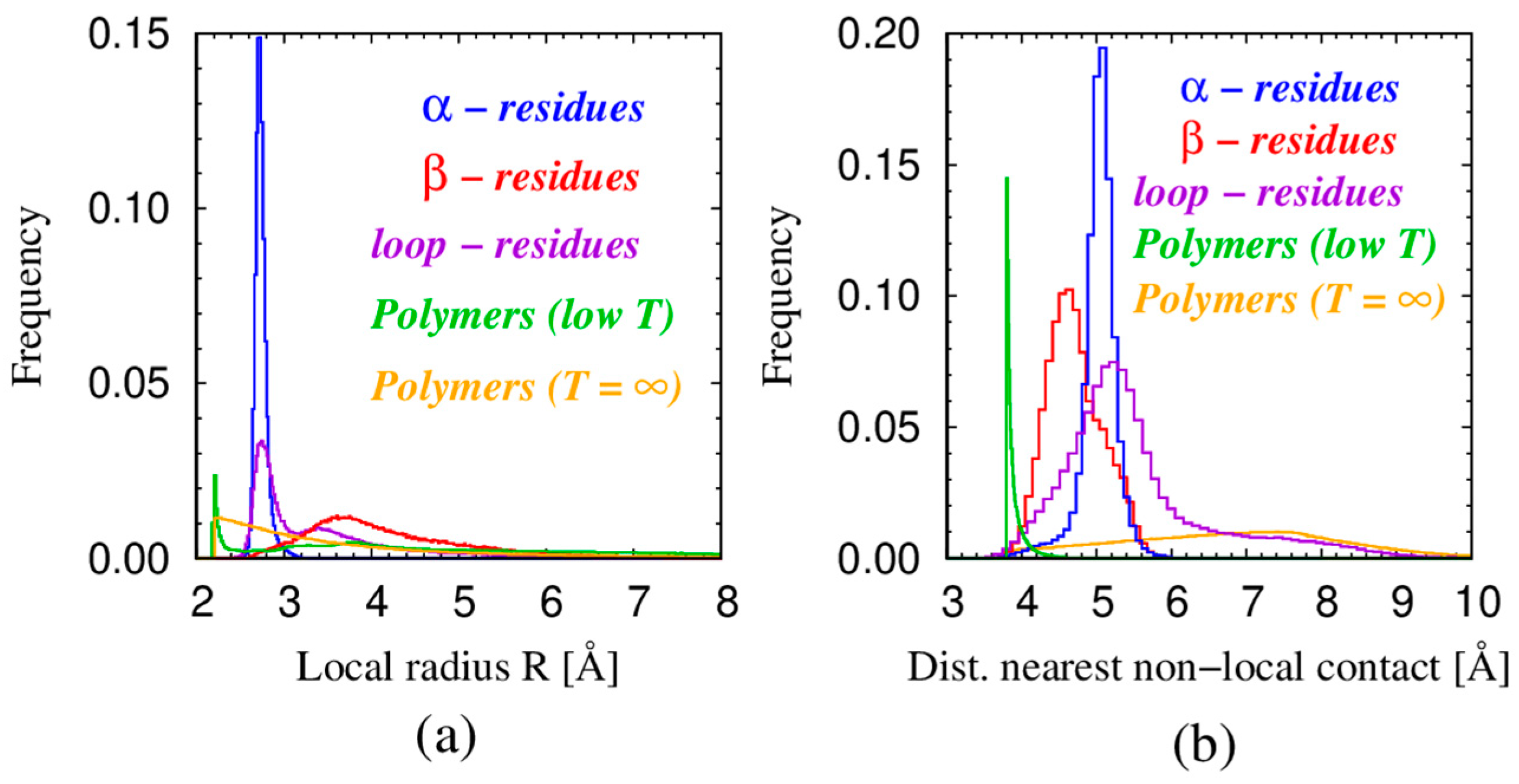
| Monomers | Most Frequent Value of Local Radius [Å] | Relevant Non-Local Length Scale [Å] |
|---|---|---|
| α—residues in proteins | 2.73 | 5.06 |
| β—residues in proteins | 3.6 | 4.67 |
| loop—residues in proteins | 2.75 | 5.26 |
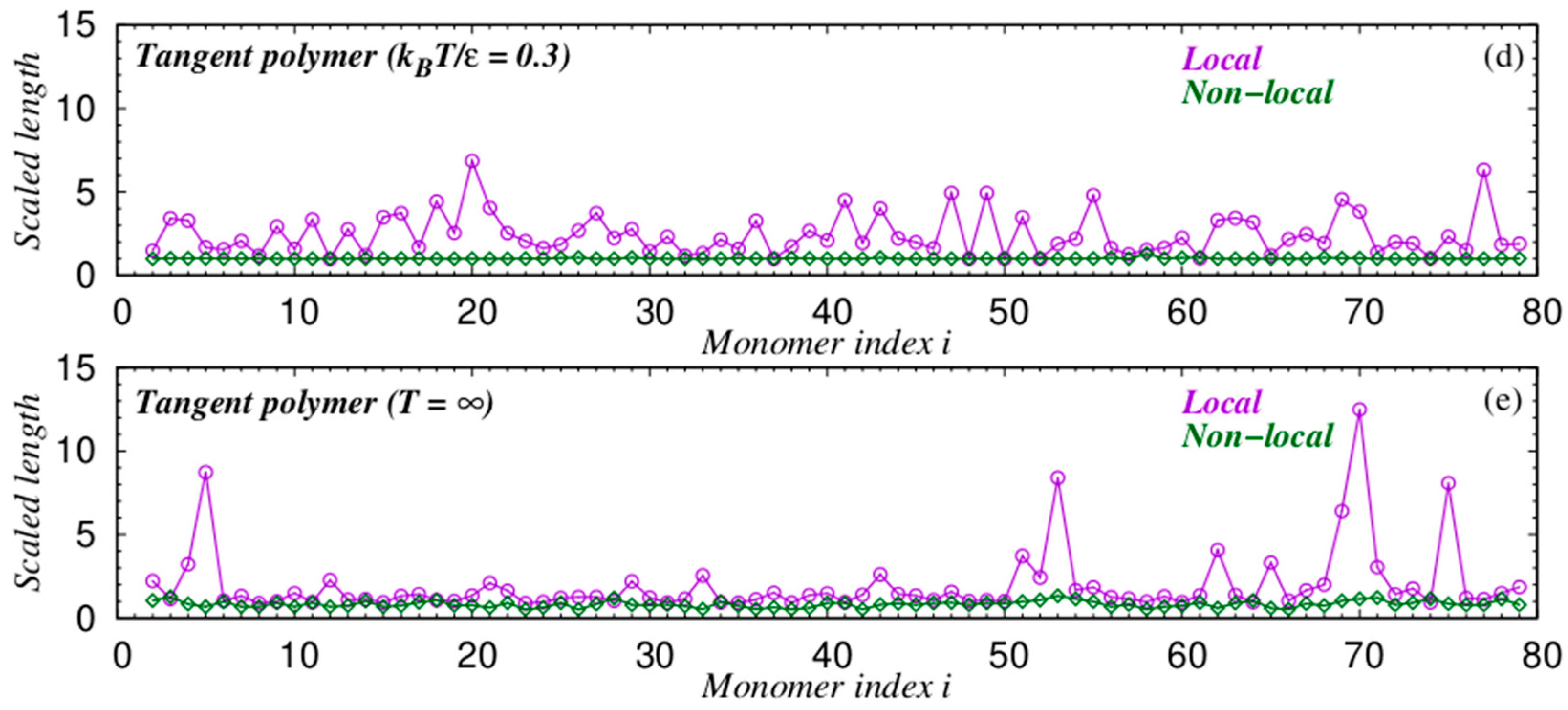
| Spheres in tangent polymers at low T | 2.21 | 3.81 |
| Spheres in tangent polymers at T = ∞ | 2.47 | 7.72 |
Disclaimer/Publisher’s Note: The statements, opinions and data contained in all publications are solely those of the individual author(s) and contributor(s) and not of MDPI and/or the editor(s). MDPI and/or the editor(s) disclaim responsibility for any injury to people or property resulting from any ideas, methods, instructions or products referred to in the content. |
© 2024 by the authors. Licensee MDPI, Basel, Switzerland. This article is an open access article distributed under the terms and conditions of the Creative Commons Attribution (CC BY) license (https://creativecommons.org/licenses/by/4.0/).
Share and Cite
Škrbić, T.; Giacometti, A.; Hoang, T.X.; Maritan, A.; Banavar, J.R. A Tale of Two Chains: Geometries of a Chain Model and Protein Native State Structures. Polymers 2024, 16, 502. https://doi.org/10.3390/polym16040502
Škrbić T, Giacometti A, Hoang TX, Maritan A, Banavar JR. A Tale of Two Chains: Geometries of a Chain Model and Protein Native State Structures. Polymers. 2024; 16(4):502. https://doi.org/10.3390/polym16040502
Chicago/Turabian StyleŠkrbić, Tatjana, Achille Giacometti, Trinh X. Hoang, Amos Maritan, and Jayanth R. Banavar. 2024. "A Tale of Two Chains: Geometries of a Chain Model and Protein Native State Structures" Polymers 16, no. 4: 502. https://doi.org/10.3390/polym16040502
APA StyleŠkrbić, T., Giacometti, A., Hoang, T. X., Maritan, A., & Banavar, J. R. (2024). A Tale of Two Chains: Geometries of a Chain Model and Protein Native State Structures. Polymers, 16(4), 502. https://doi.org/10.3390/polym16040502