
A Novel High Recognition Rate Defect Inspection Method for Carbon Fiber Plain-Woven Prepreg Based on Image Texture Feature Compression


Abstract
:1. Introduction
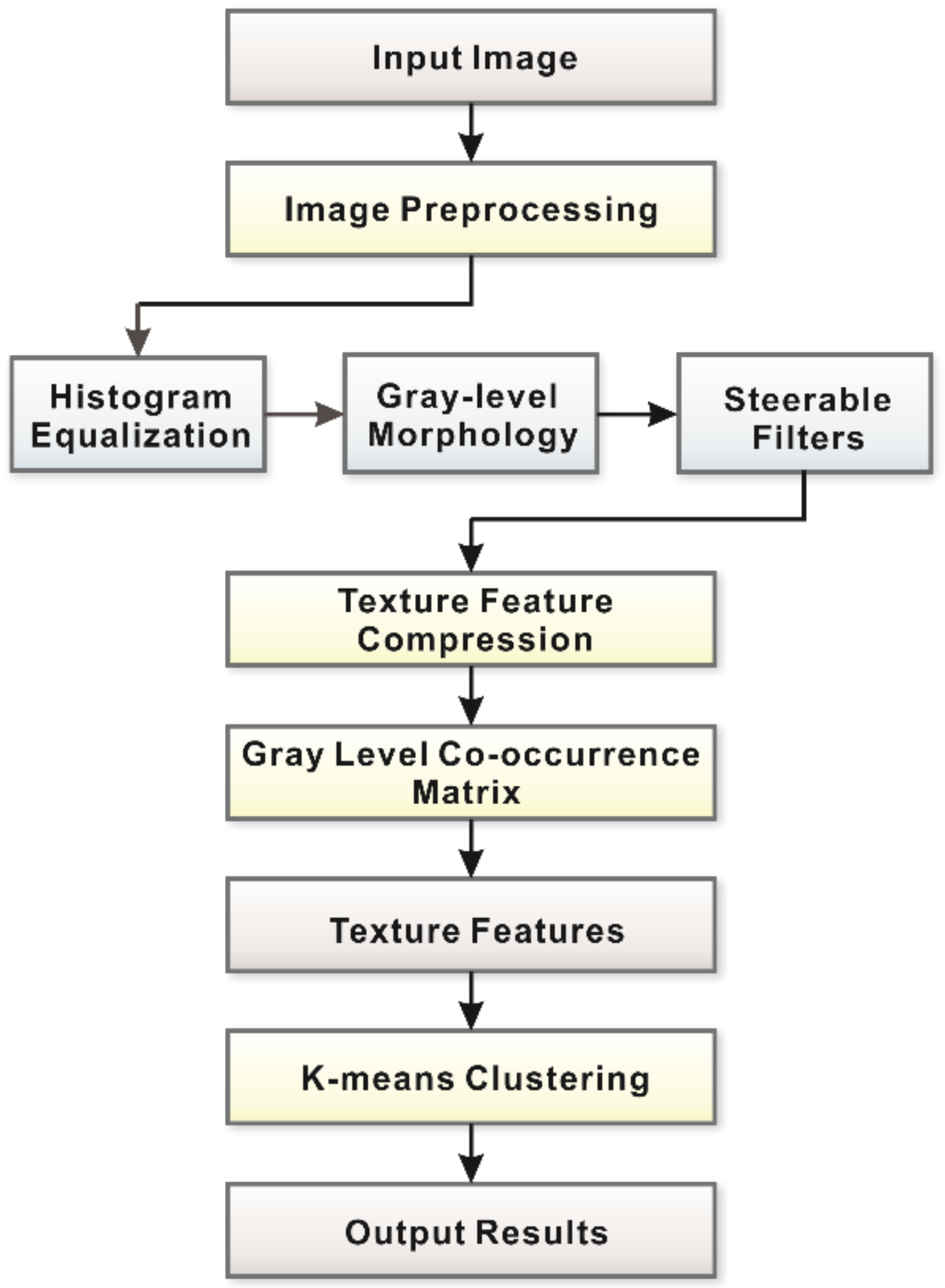
2. Methodology
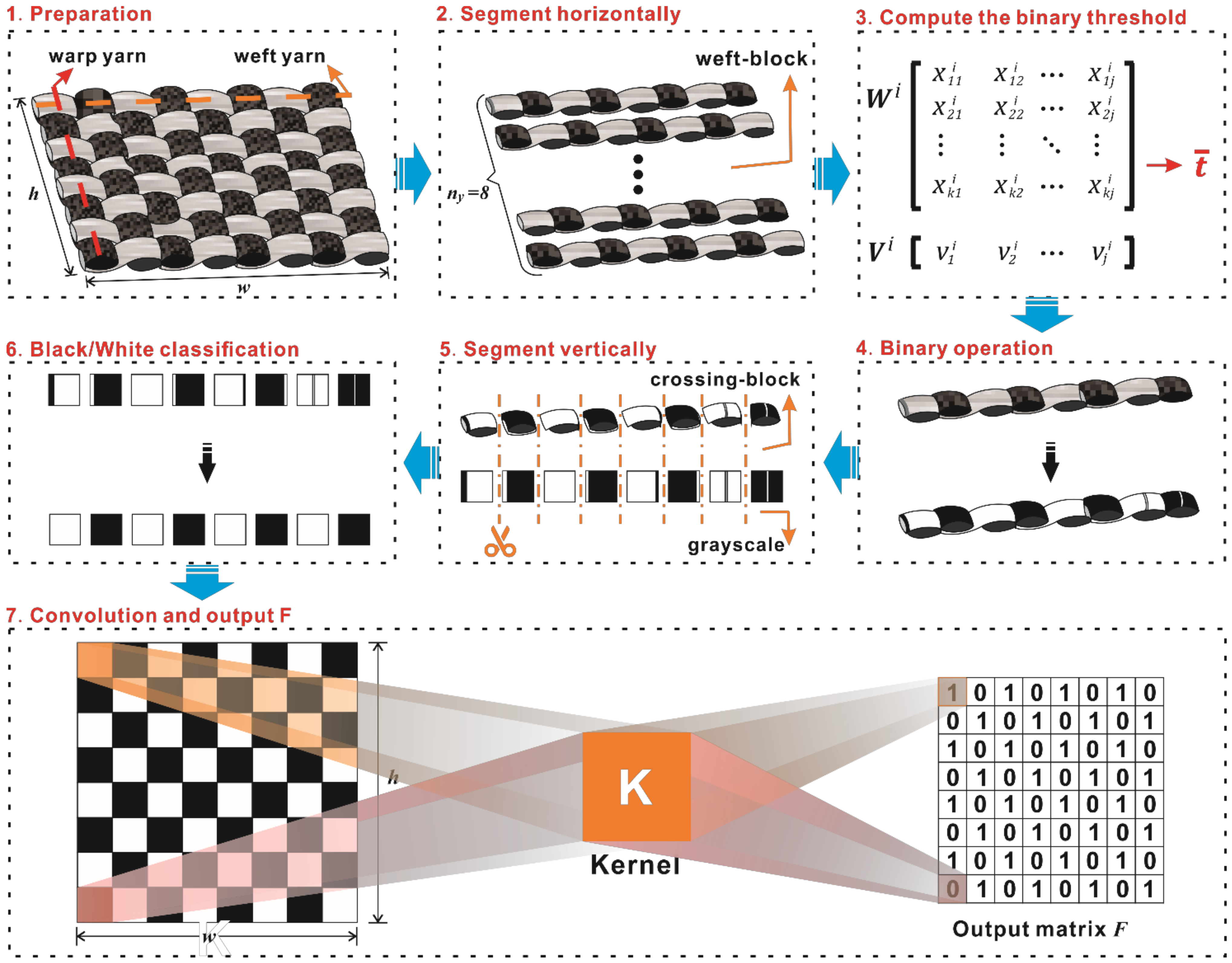
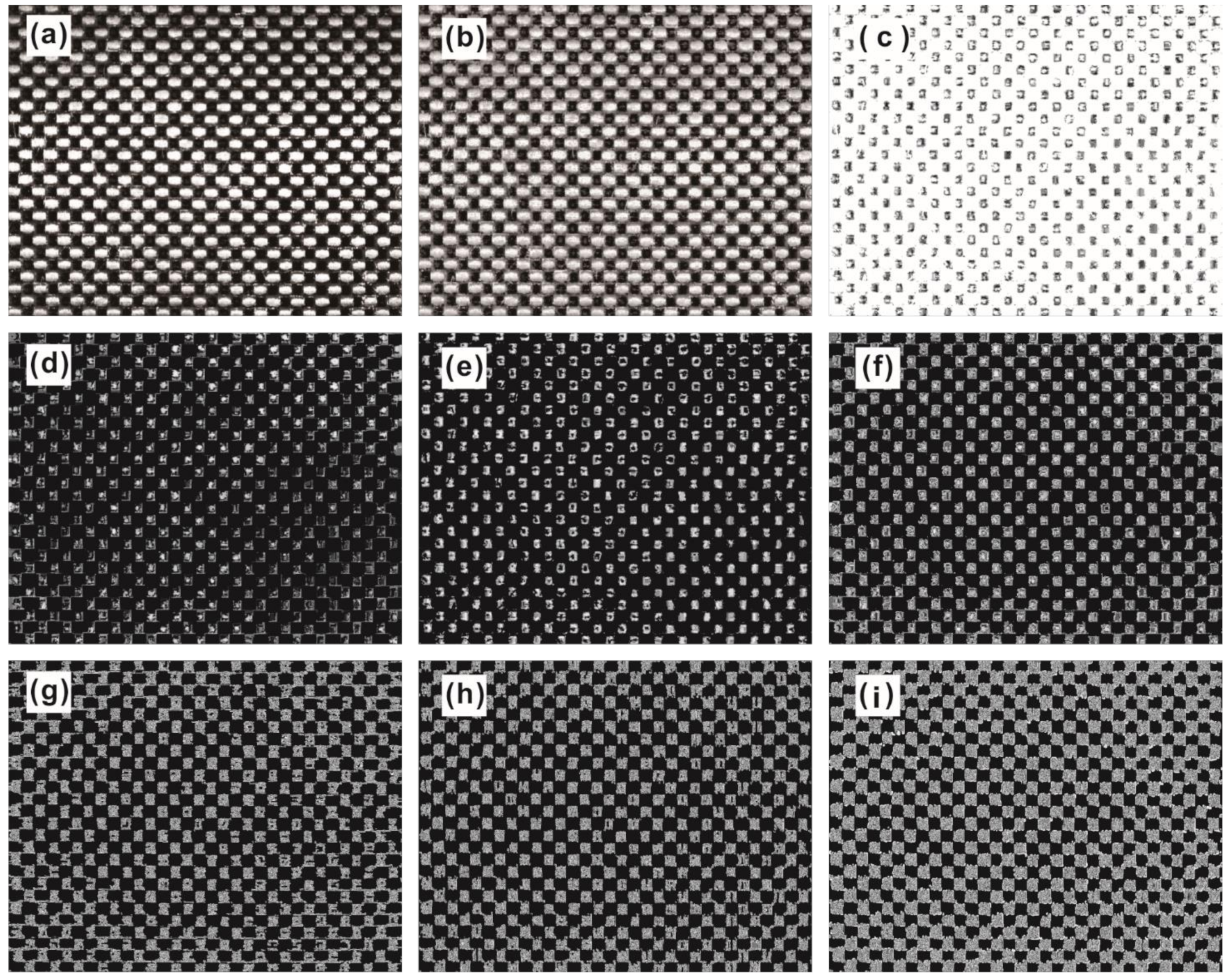
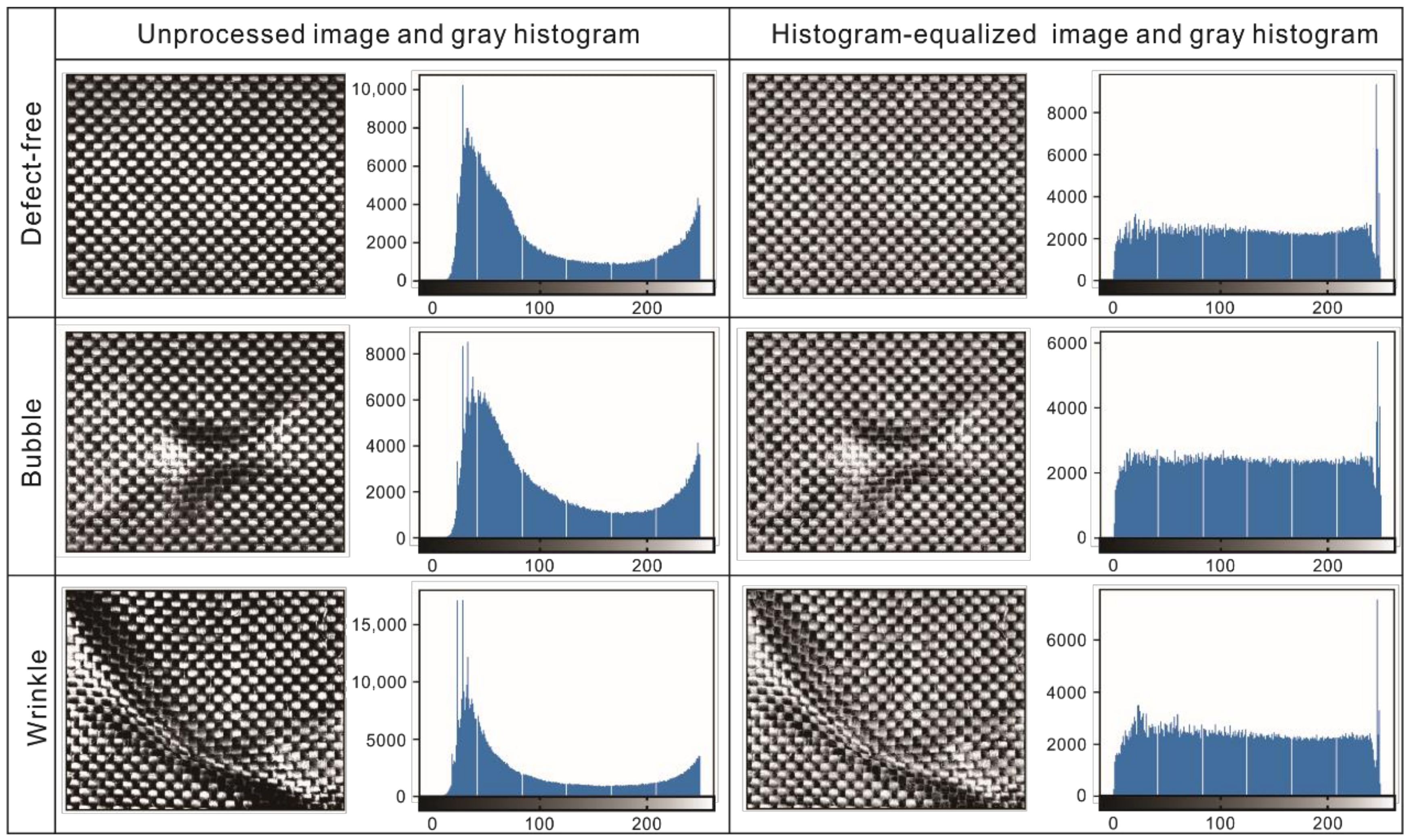
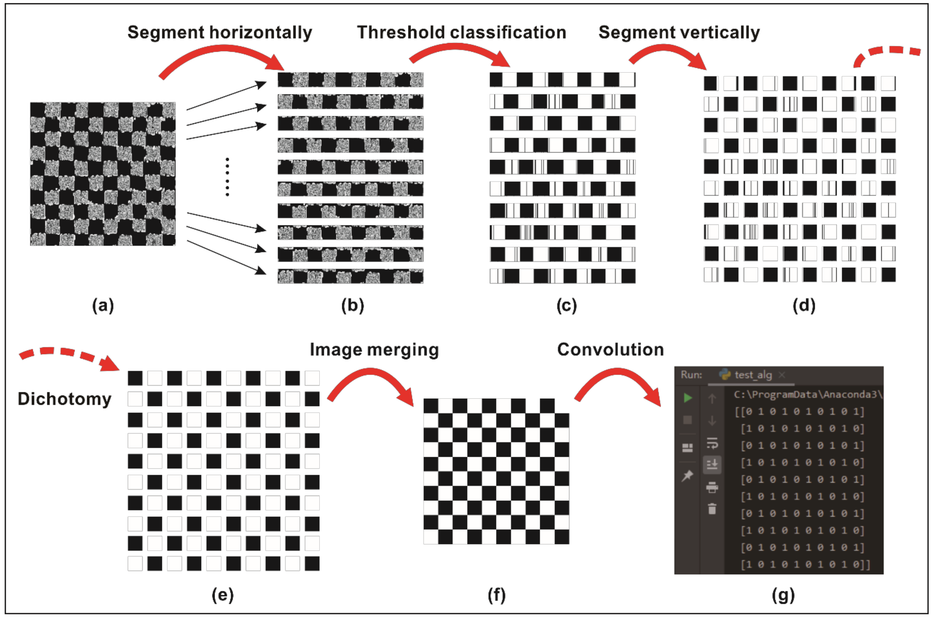
2.1. Image Preprocessing
2.2. Image Compression
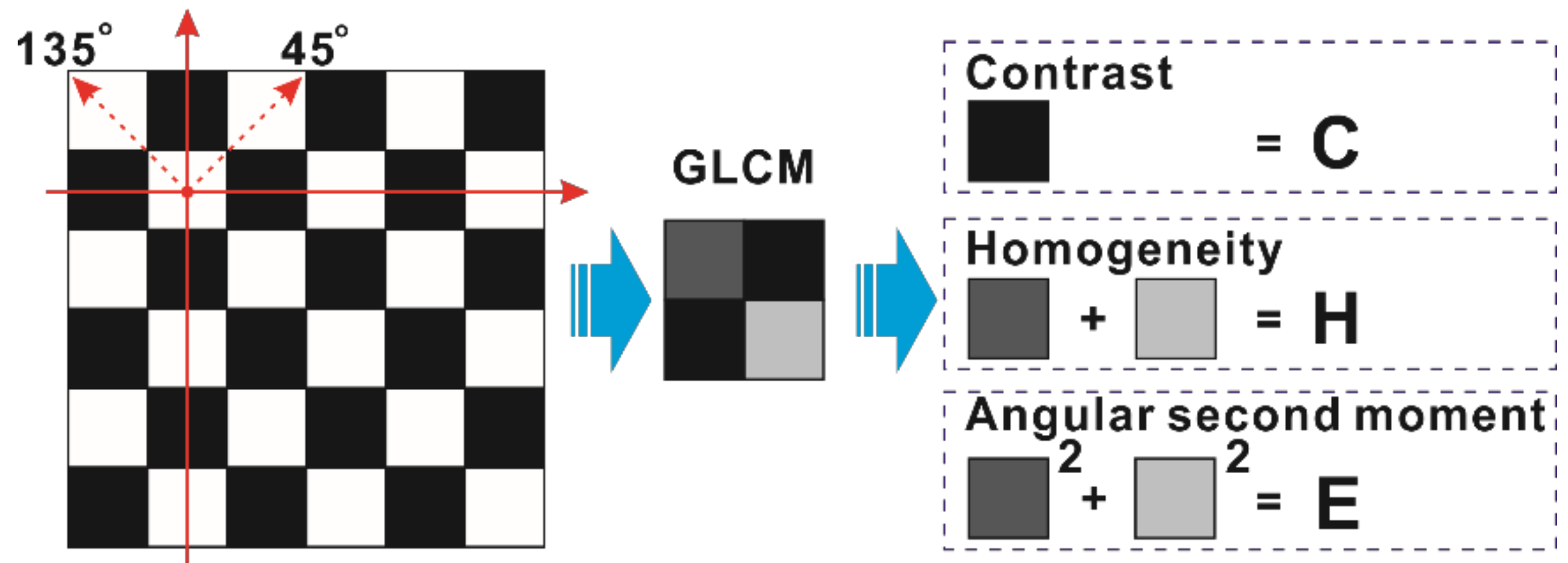
2.3. Texture Feature Extraction
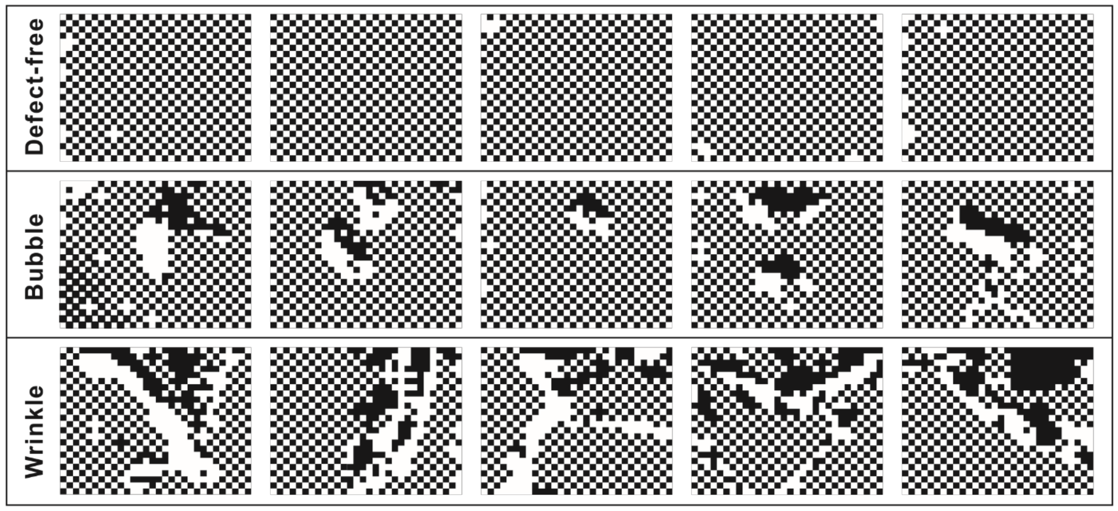
2.4. Defect Inspection
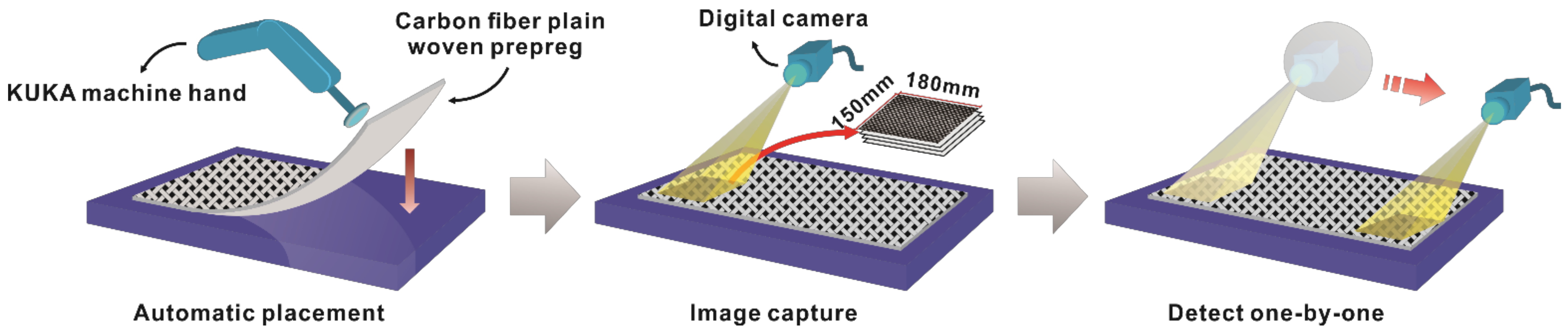
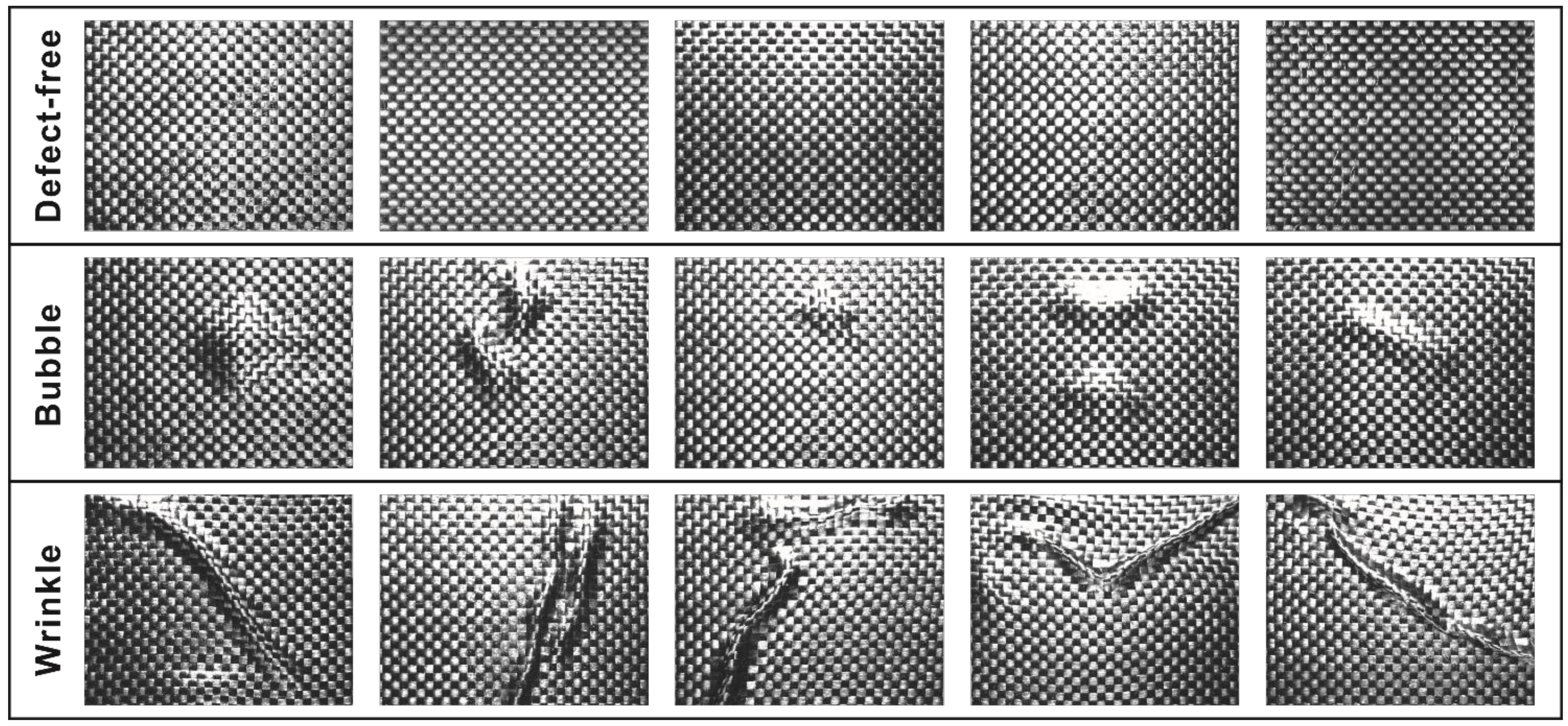
3. Materials and Experiments
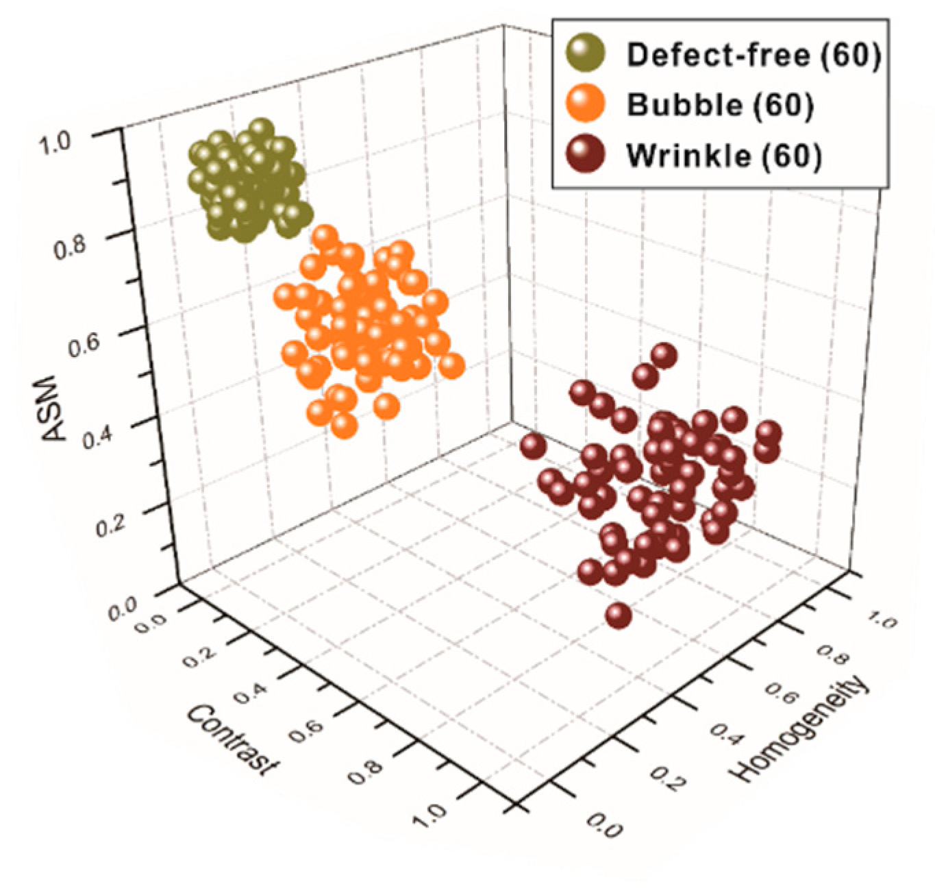
4. Results and Discussion
5. Conclusions
Author Contributions
Funding
Institutional Review Board Statement
Informed Consent Statement
Data Availability Statement
Conflicts of Interest
Nomenclature
| Oorg | original image matrix |
| w | image width (px) |
| h | image height (px) |
| nx | the numbers of warps |
| ny | the numbers of wefts |
| Wi | weft-block matrix |
| binary threshold value | |
| Obnr | binary matrix |
| Cil | crossing-block matrix |
| F | output matrix |
| Mij | co-occurrence matrix |
| C | contrast |
| H | homogeneity |
| E | angular second moment |
Appendix A
- (1)
- Histogram equalization: Firstly, the global image is equalized directly. Suppose that the histogram distribution of the captured image A is HA(D). The monotone nonlinear mapping is used to change image A into image B, that is, function transformation f is applied to each pixel in image A, and the histogram of image B is obtained as HB(D).
- (2)
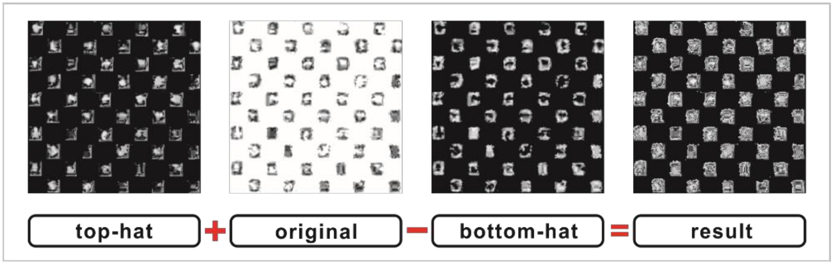
- Gray-level morphology: The operation object of gray-level mathematical morphology is not a set, but an image function. The dilation and erosion operations of the input image f(x, y) with structure element b(x, y) are respectively defined as:
- (3)
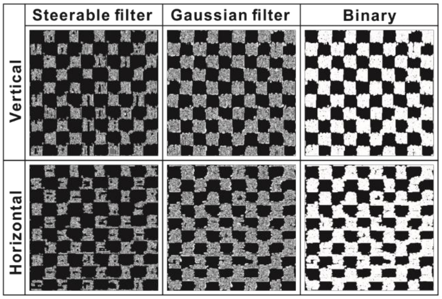
- Steerable filters: Considering the woven pattern, we use the steerable vertical filters with the following basic 2-D Gaussian function in this paper.where σx and σy are the standard deviation in the x and y directions, respectively.
- (4)
- Performance evaluation metrics: First, the numerical comparisons between steerable filtered images (binary images after filter) and template images are conducted in a pixel-by-pixel manner. Specifically, both pixel values in the filtered and template images are 255 as true positive (TP), while 0 as true negative (TN). The pixel value in the filtered image is 255 and that of the defect manual-labeled image is 0 as false positive (FP), while the reversed situation is false negative (FN). The following measurement metrics are used to compare the result of applying vertical and horizontal steerable filters:
- (5)
- Gray level co-occurrence matrix: All values of the co-occurrence matrices are given normalized treatment before the texture features are calculated. The co-occurrence matrices, Mij, is shown as Equation (A22).
References
- Zhang, J.; Chaisombat, K.; He, S.; Wang, C.H. Hybrid composite laminates reinforced with glass/carbon woven fabrics for lightweight load bearing structures. Mater. Des. 2018, 36, 75–80. [Google Scholar] [CrossRef]
- Deng, B.; Shi, Y.; Yu, T.; Zhao, P. Influence mechanism and optimization analysis of technological parameters for the composite prepreg tape winding process. Polymers 2020, 12, 1843. [Google Scholar] [CrossRef] [PubMed]
- Tan, Y.; Meng, L.; Zhang, D. Strain sensing characteristic of ultrasonic excitation-fiber Bragg gratings damage detection technique. Measurement 2013, 46, 294–304. [Google Scholar] [CrossRef]
- Crane, R.L.; Chang, F.F.; Allinikov, S. Use of radiographically opaque fibers to aid the inspection of composites. Mater. Eval. 1978, 36, 69–71. [Google Scholar]
- Addepalli, S.; Zhao, Y.; Roy, R.; Galhenege, W.; Colle, M.; Yu, J.; Ucur, A. Non-destructive evaluation of localised heat damage occurring in carbon composites using thermography and thermal diffusivity measurement. Measurement 2019, 131, 706–713. [Google Scholar] [CrossRef]
- Aisyah, H.A.; Tahir, P.M.; Sapuan, S.M.; Ilyas, R.A.; Khalina, A.; Nurazzi, N.M.; Lee, S.H.; Lee, C.H. A comprehensive review on advanced sustainable woven natural fibre polymer composites. Polymers 2021, 13, 471. [Google Scholar] [CrossRef]
- Hanbay, K.; Talu, M.F.; Ozguven, O.F. Fabric defect detection systems and methods-A systematic literature review. Optik 2016, 127, 11960–11973. [Google Scholar] [CrossRef]
- Ngan, H.Y.T.; Pang, G.K.H.; Yung, N.H.C. Automated fabric defect detection—A review. Image Vis. Comput. 2011, 29, 442–458. [Google Scholar] [CrossRef]
- Song, K.Y.; Kittler, J.; Petrou, M. Defect detection in random colour textures. Image Vis. Comput. 1996, 14, 667–683. [Google Scholar] [CrossRef]
- Bodnarova, A.; Bennamoun, M.; Kubik, K.K. Defect detection in textile materials based on aspects of the HVS. In Proceedings of the 1998 IEEE International Conference on Systems, Man, and Cybernetics, San Diego, CA, USA, 14 October 1998; Volume 5, pp. 4423–4428. [Google Scholar]
- Tabassian, M.; Ghaderi, R.; Ebrahimpour, R. Knitted fabric defect classification for uncertain labels based on Dempster-Shafer theory of evidence. Expert Syst. Appl. 2011, 38, 5259–5267. [Google Scholar] [CrossRef]
- Tong, L.; Wong, W.K.; Kwong, C.K. Differential evolution-based optimal Gabor filter model for fabric inspection. Neurocomputing 2016, 173, 1386–1401. [Google Scholar] [CrossRef]
- Tsai, D.M.; Hsieh, C.Y. Automated surface inspection for directional textures. Image Vis. Comput. 1999, 18, 49–62. [Google Scholar] [CrossRef]
- Alata, O.; Ramananjarasoa, C. Unsupervised textured image segmentation using 2-D quarter plane autoregressive model with four prediction supports. Pattern Recognit. Lett. 2005, 26, 1069–1081. [Google Scholar] [CrossRef]
- Bouhamidi, A.; Jbilou, K. An iterative method for Bayesian Gauss-Markov image restoration. Appl. Math. Model. 2009, 33, 361–372. [Google Scholar] [CrossRef]
- Monaco, J.P.; Madabhushi, A. Class-specific weighting for Markov random field estimation: Application to medical image segmentation. Med. Image Anal. 2012, 16, 1477–1489. [Google Scholar] [CrossRef] [PubMed] [Green Version]
- Zhang, Y.X.F.; Bresee, R.R. Fabric defect detection and clssification using image-analysis. Text. Res. J. 1995, 65, 1–9. [Google Scholar] [CrossRef]
- Latif-Amet, A.; Ertuzun, A.; Ercil, A. An efficient method for texture defect detection: Sub-band domain co-occurrence matrices. Image Vis. Comput. 2000, 18, 543–553. [Google Scholar] [CrossRef]
- Ng, H.F. Automatic thresholding for defect detection. Pattern Recognit. Lett. 2006, 27, 1644–1649. [Google Scholar] [CrossRef]
- Jia, L.; Liang, J.Z. Fabric defect inspection based on isotropic lattice segmentation. J. Frankl. Inst. Eng. Appl. Math. 2017, 354, 5694–5738. [Google Scholar] [CrossRef]
- Ng, M.K.; Ngan, H.Y.T.; Yuan, X.M.; Zhang, W.X. Patterned fabric inspection and visualization by the method of image decomposition. IEEE Trans. Autom. Sci. Eng. 2014, 11, 943–947. [Google Scholar] [CrossRef] [Green Version]
- Ngan, H.Y.T.; Pang, G.K.H.; Yung, N.H.C. Motif-based defect detection for patterned fabric. Pattern Recognit. 2008, 41, 1878–1894. [Google Scholar] [CrossRef]
- Ngan, H.Y.T.; Pang, G.K.H. Novel method for patterned fabric inspection using Bollinger bands. Opt. Eng. 2006, 45, 087202. [Google Scholar]
- Ngan, H.Y.T.; Pang, G.K.H. Regularity analysis for patterned texture inspection. IEEE Trans. Autom. Sci. Eng. 2009, 6, 131–144. [Google Scholar] [CrossRef] [Green Version]
- Tsang, C.S.C.; Ngan, H.Y.T.; Pang, G.K.H. Fabric inspection based on the Elo rating method. Pattern Recognit. 2016, 51, 378–394. [Google Scholar] [CrossRef] [Green Version]
- Ngan, H.Y.T.; Pang, G.K.H.; Yung, S.P.; Ng, M.K. Wavelet based methods on patterned fabric defect detection. Pattern Recognit. 2005, 38, 559–576. [Google Scholar] [CrossRef]
- Starck, J.L.; Elad, M.; Donoho, D. Redundant multiscale transforms and their application for morphological component separation. Adv. Imag. Elect. Phys. 2004, 132, 287–348. [Google Scholar]
- Xu, L.; Yan, Q.; Xia, Y.; Jia, J.Y. Structure extraction from texture via relative total variation. ACM Trans. Graph. 2012, 31, 1–10. [Google Scholar] [CrossRef]
- Ng, M.K.; Yuan, X.M.; Zhang, W.X. Coupled variational image decomposition and restoration model for blurred cartoon-plus-texture images with missing pixels. IEEE Trans. Image Process. 2013, 22, 2233–2246. [Google Scholar] [CrossRef]
- Jia, L.; Chen, C.; Xu, S.K.; Shen, J. Fabric defect inspection based on lattice segmentation and template statistics. Inf. Sci. 2020, 512, 964–984. [Google Scholar] [CrossRef]
- Zhang, H.M.; Pei, Z.L.; Zhang, Z.G. Design and implementation of image processing system based on MATLAB. In Proceedings of the International Conference on Logistics Engineering, Management and Computer Science, Shenyang, China, 19 July 2015; Volume 117, pp. 1356–1359. [Google Scholar]
- Wang, T.T.; Dong, J.C. Application of image enhancement in the electronation of ancient books. Nat. Sci. Ed. 2015, 33, 26–29. [Google Scholar]
- Haralick, R.M. Statistical and structural approaches to texture. Proc. IEEE 1979, 67, 786–804. [Google Scholar] [CrossRef]
- Soh, L.K.; Tsatsoulis, C. Texture analysis of SAR sea ice imagery using gray level co-occurrence matrices. IEEE Trans. Geosci. Remote Sens. 1999, 37, 780–795. [Google Scholar] [CrossRef] [Green Version]
- Xin, B.; Zhang, J.; Zhang, R.; Wu, X. Color texture classification of yarn-dyed woven fabric based on dual-side scanning and co-occurrence matrix. Text. Res. J. 2017, 87, 1883–1895. [Google Scholar] [CrossRef]
- Baralidi, A.; Parmiggian, F. An investigation of the textural characteristics associated with gray level cooccurrence matrix statistical parameters. IEEE Trans. 1995, 33, 293–303. [Google Scholar]
- Kuo, C.F.J.; Tsai, C.C. Automatic recognition of fabric nature by using the approach of texture analysis. Text. Res. J. 2006, 76, 375–382. [Google Scholar] [CrossRef]
- Du, Z.; Gao, R.; Zhou, T.; He, L. Determination of featured parameters to cluster stiffness handle of fabrics by the CHES-FY system. Fiber. Polym. 2013, 14, 1768–1775. [Google Scholar] [CrossRef]
- Likas, A.; Vlassis, N.; Verbeek, J.J. The global k-means clustering algorithm. Pattern Recognit. 2003, 36, 451–461. [Google Scholar] [CrossRef] [Green Version]
- Mei, S.; Yang, H.; Yin, Z. An unsupervised-learning-based approach for automated defect inspection on textured surfaces. IEEE Trans. Instrum. Meas. 2018, 67, 1266–1277. [Google Scholar] [CrossRef]
- Li, Y.; Zhao, W.; Pan, J. Deformable patterned fabric defect detection with fisher criterion-based deep learning. IEEE Trans. Autom. Sci. Eng. 2017, 14, 1256–1264. [Google Scholar] [CrossRef]
- Zhang, K.; Li, P.; Dong, A.; Zhang, K. Yarn-dyed fabric defect classification based on convolutional neural network. Opt. Eng. 2017, 56, 093104. [Google Scholar]


| Function | Position | Conditions |
|---|---|---|
| M (i, j, d, 45°) | RRD(d): (x1 − x2= d, y1 − y2= −d) or (x1 − x2= -d, y1 − y2= d) | {RRD(d), f(x1, y1) = i, f(x2, y2) = j} |
| M (i, j, d, 135°) | RLD(d): (x1 − x2= d, y1 − y2= d) or (x1 − x2= -d, y1 − y2= −d) | {RLD(d), f(x1, y1) = i, f(x2, y2) = j} |
| Image Size | Direction | ACC | TPR | FPR | PPV | NPV |
|---|---|---|---|---|---|---|
| 10 × 10 | Vertical | 82.27 | 78.13 | 13.31 | 86.27 | 78.74 |
| Horizontal | 72.89 | 72.24 | 26.39 | 74.71 | 71.07 | |
| Full-size | Vertical | 77.33 | 69.57 | 19.29 | 81.43 | 73.36 |
| Horizontal | 63.58 | 36.49 | 47.33 | 90.01 | 56.19 |
| Specimens | Contrast | Homogeneity | Angular Second Moment |
|---|---|---|---|
| Defect-free | 0.032 | 0.022 | 0.960 |
| Bubble | 0.272 | 0.242 | 0.680 |
| Wrinkle | 0.839 | 0.830 | 0.177 |
| Defect-Free: Bubble: Wrinkle | Defect-Free Cluster Center Coordinates | Bubble Cluster Center Coordinates | Wrinkle Cluster Center Coordinates |
|---|---|---|---|
| 2:3:5 | (0.0352, 0.0225, 0.9556) | (0.2746, 0.2456, 0.6734) | (0.8345, 0.9934, 0.1579) |
| 2:4:4 | (0.0352, 0.0225, 0.9556) | (0.2746, 0.2456, 0.6734) | (0.8345, 0.9934, 0.1579) |
| 2:5:3 | (0.0352, 0.0225, 0.9556) | (0.2746, 0.2456, 0.6734) | (0.8345, 0.9934, 0.1579) |
| Defect-Free: Bubble: Wrinkle | Defect-Free Cluster Center Coordinates | Bubble Cluster Center Coordinates | Wrinkle Cluster Center Coordinates |
|---|---|---|---|
| 2:3:5 | (0.0321, 0.0203, 0.9596) | (0.2696, 0.2425, 0.6759) | (0.8389, 0.8297, 0.1779) |
| 2:4:4 | (0.0322, 0.0217, 0.9598) | (0.2719, 0.2427, 0.6799) | (0.8393, 0.8304, 0.1773) |
| 2:5:3 | (0.0319, 0.0221, 0.9603) | (0.2734, 0.2408, 0.6811) | (0.8432, 0.8314, 0.1763) |
| Proportion | TN/TB/TW | RN/RB/RW | IN/% | IB/% | IW/% | IM/% | IE/% |
|---|---|---|---|---|---|---|---|
| 2:3:5 | 200:300:500 | 188:283:471 | 94.00 | 94.33 | 94.20 | 94.18 | 94.41 |
| 2:4:4 | 200:400:400 | 189:379:380 | 94.50 | 94.75 | 95.00 | 94.75 | |
| 2:5:3 | 200:500:300 | 189:469:284 | 94.50 | 93.80 | 94.67 | 94.32 |
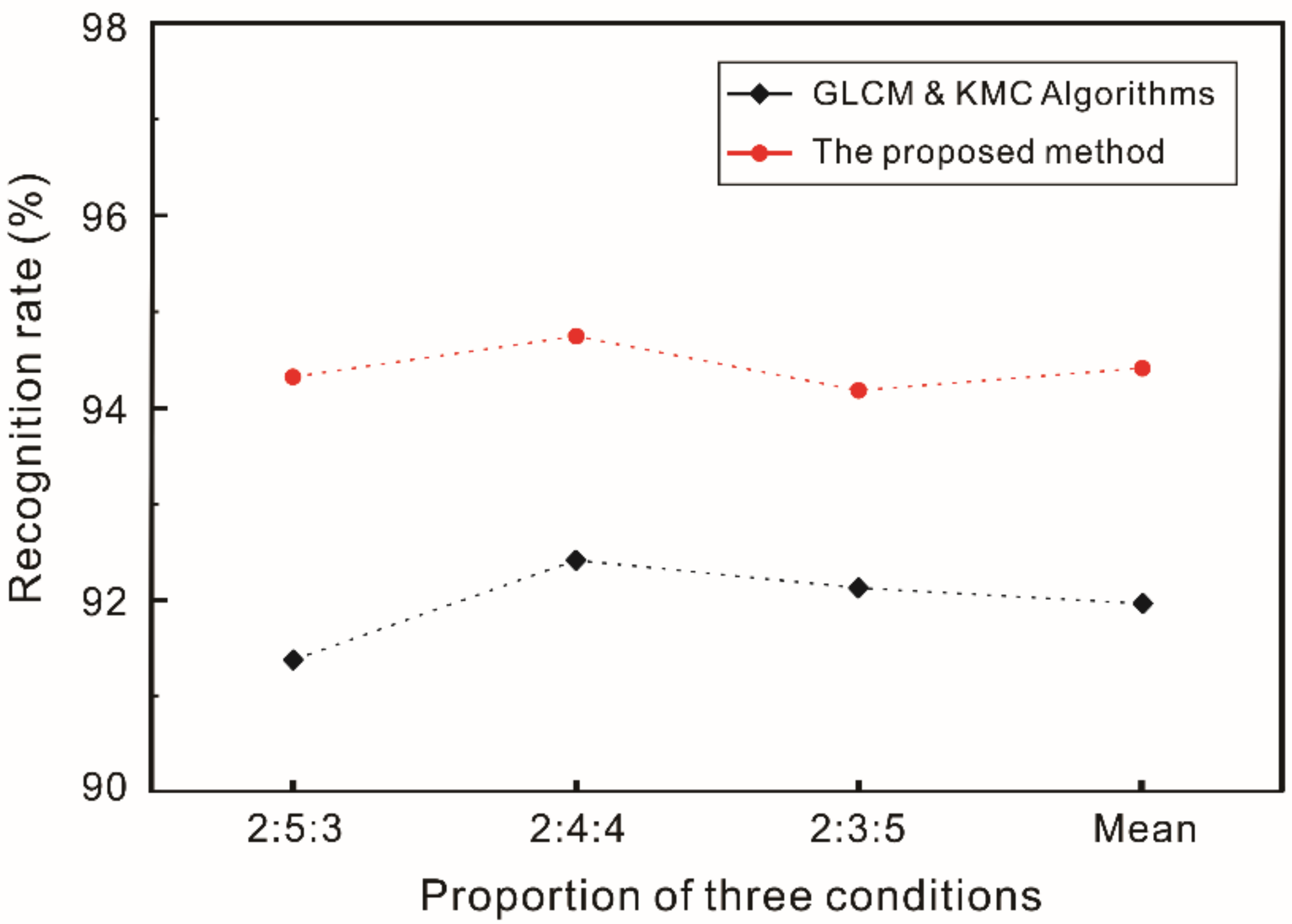
| Data Set | Proportion | Recognition Accuracy (%) | Average Value (%) |
|---|---|---|---|
| 1 | 2:3:5 | 92.12 | 91.96 |
| 2 | 2:4:4 | 92.41 | |
| 3 | 2:5:3 | 91.37 |
| Method | GLCM & KMC Method | The Proposed Method of This Article |
|---|---|---|
| Each testing time (ms) | 472 | 136 |
| Total testing time (min) | 7.87 | 2.27 |
Publisher’s Note: MDPI stays neutral with regard to jurisdictional claims in published maps and institutional affiliations. |
© 2022 by the authors. Licensee MDPI, Basel, Switzerland. This article is an open access article distributed under the terms and conditions of the Creative Commons Attribution (CC BY) license (https://creativecommons.org/licenses/by/4.0/).
Share and Cite
Li, L.; Wang, Y.; Qi, J.; Xiao, S.; Gao, H. A Novel High Recognition Rate Defect Inspection Method for Carbon Fiber Plain-Woven Prepreg Based on Image Texture Feature Compression. Polymers 2022, 14, 1855. https://doi.org/10.3390/polym14091855
Li L, Wang Y, Qi J, Xiao S, Gao H. A Novel High Recognition Rate Defect Inspection Method for Carbon Fiber Plain-Woven Prepreg Based on Image Texture Feature Compression. Polymers. 2022; 14(9):1855. https://doi.org/10.3390/polym14091855
Chicago/Turabian StyleLi, Lun, Yiqi Wang, Jialiang Qi, Shenglei Xiao, and Hang Gao. 2022. "A Novel High Recognition Rate Defect Inspection Method for Carbon Fiber Plain-Woven Prepreg Based on Image Texture Feature Compression" Polymers 14, no. 9: 1855. https://doi.org/10.3390/polym14091855
APA StyleLi, L., Wang, Y., Qi, J., Xiao, S., & Gao, H. (2022). A Novel High Recognition Rate Defect Inspection Method for Carbon Fiber Plain-Woven Prepreg Based on Image Texture Feature Compression. Polymers, 14(9), 1855. https://doi.org/10.3390/polym14091855