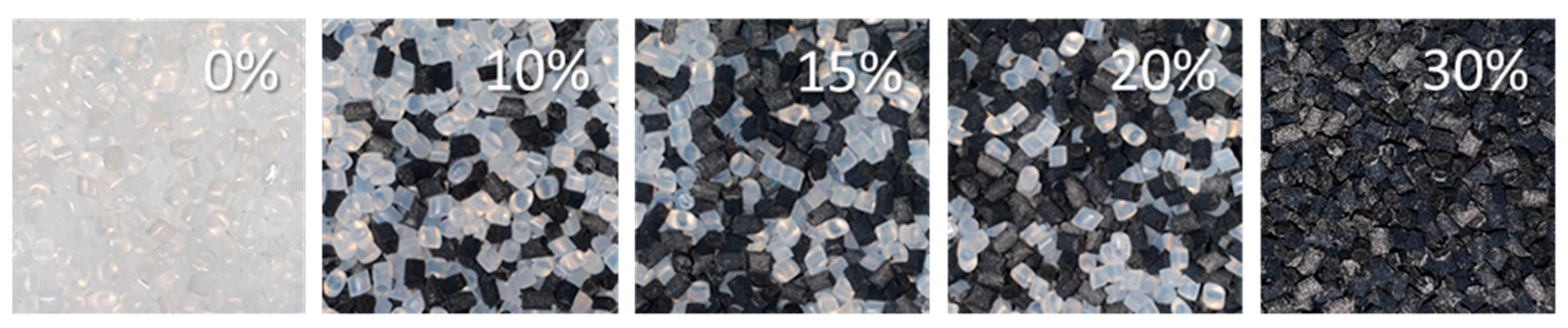
Figure 1.
Mixed pellets to obtain different fiber mass fraction.
Figure 1.
Mixed pellets to obtain different fiber mass fraction.
Figure 2.
Plate molding: (a) Size and ISO 527-2 specimen layout; (b) Example manufactured plate.
Figure 2.
Plate molding: (a) Size and ISO 527-2 specimen layout; (b) Example manufactured plate.
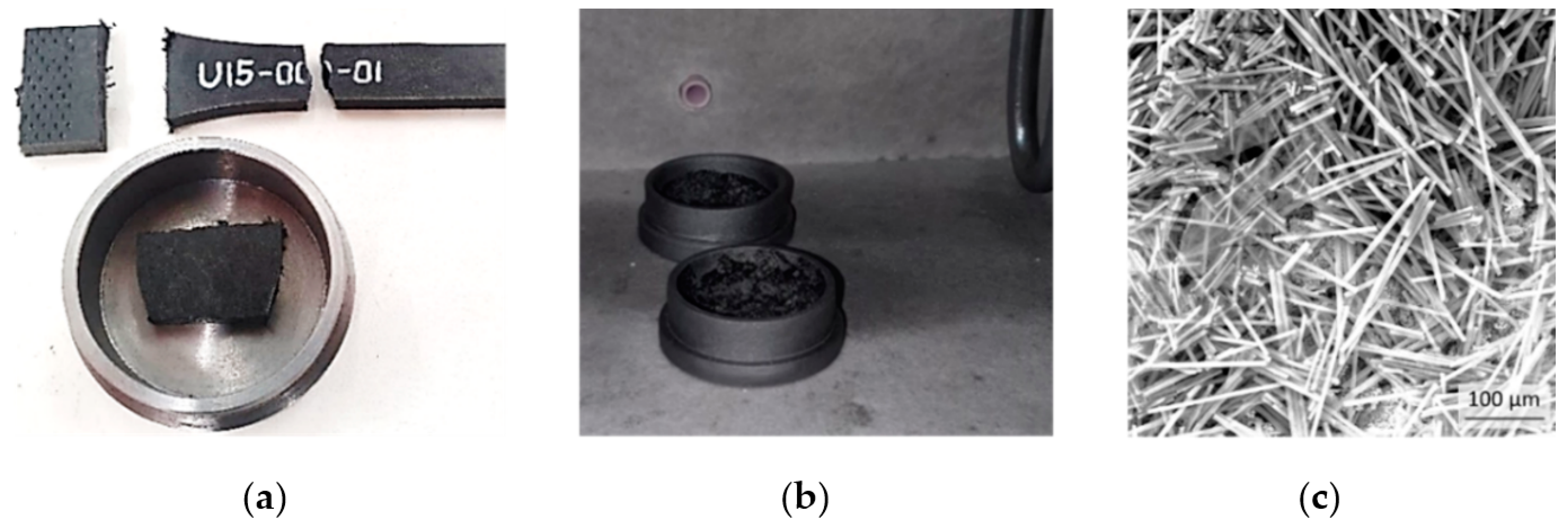
Figure 3.
Short fiber extraction from composite: (a) Sample preparation; (b) burning samples in the oven; (c) fibers after matrix burning.
Figure 3.
Short fiber extraction from composite: (a) Sample preparation; (b) burning samples in the oven; (c) fibers after matrix burning.
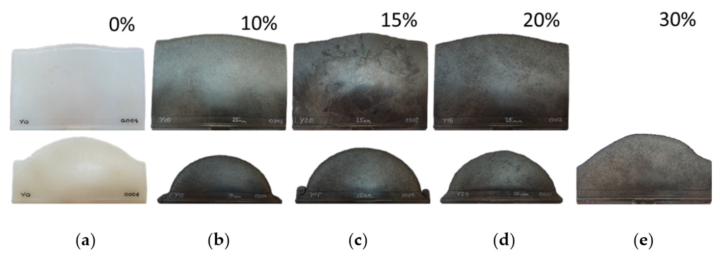
Figure 4.
Experimentally obtained plate melt front at molding composites with different fiber mass fraction: (a) 0%; (b) 10%; (c) 15%; (d) 20%; (e) 30%.
Figure 4.
Experimentally obtained plate melt front at molding composites with different fiber mass fraction: (a) 0%; (b) 10%; (c) 15%; (d) 20%; (e) 30%.
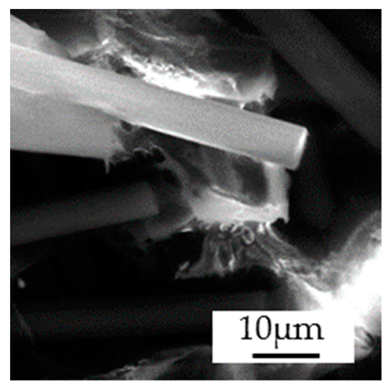
Figure 5.
Morphology of the fracture of short-fiber reinforced PA6 with 30% carbon-fiber mass fraction.
Figure 5.
Morphology of the fracture of short-fiber reinforced PA6 with 30% carbon-fiber mass fraction.
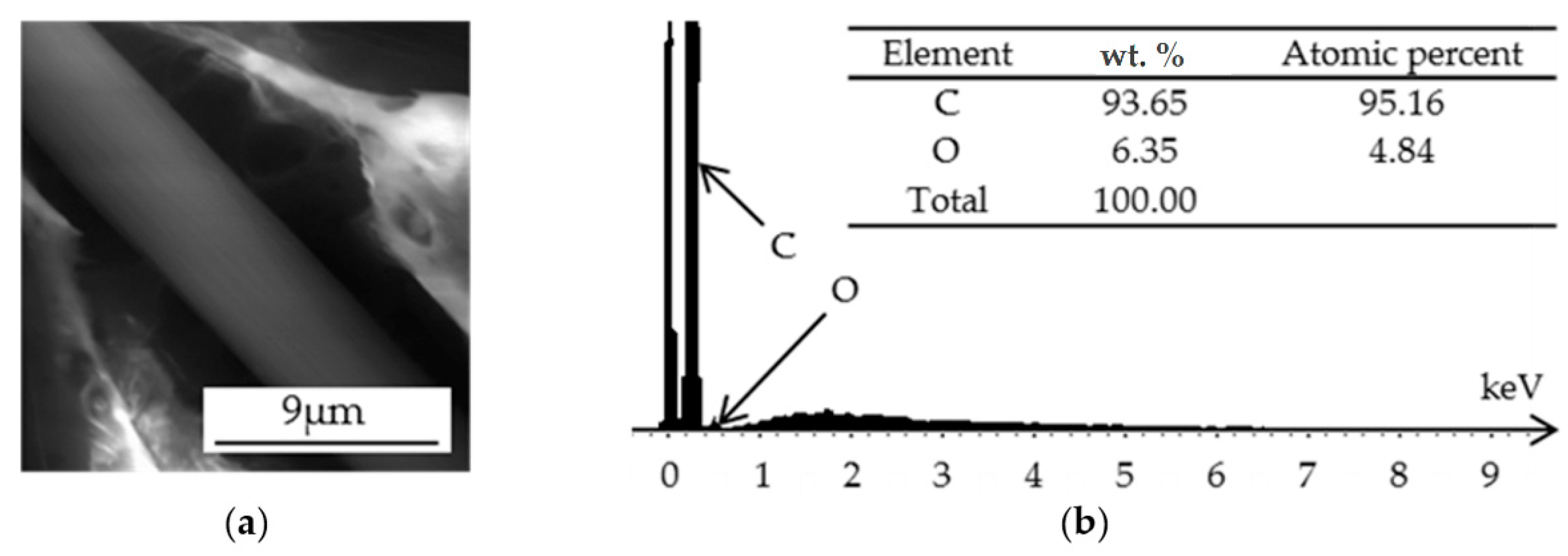
Figure 6.
Reinforced PA6 with 30 wt. % short-carbon fiber: (a) SEM; (b) XRF spectra.
Figure 6.
Reinforced PA6 with 30 wt. % short-carbon fiber: (a) SEM; (b) XRF spectra.
Figure 7.
Fracture surface of short-fiber reinforced PA6 with 15% carbon-fiber mass fraction, ISO 527-2 sample, orientated at 90°. Dashed lines demark the size in micrometers of the skin and core layer.
Figure 7.
Fracture surface of short-fiber reinforced PA6 with 15% carbon-fiber mass fraction, ISO 527-2 sample, orientated at 90°. Dashed lines demark the size in micrometers of the skin and core layer.
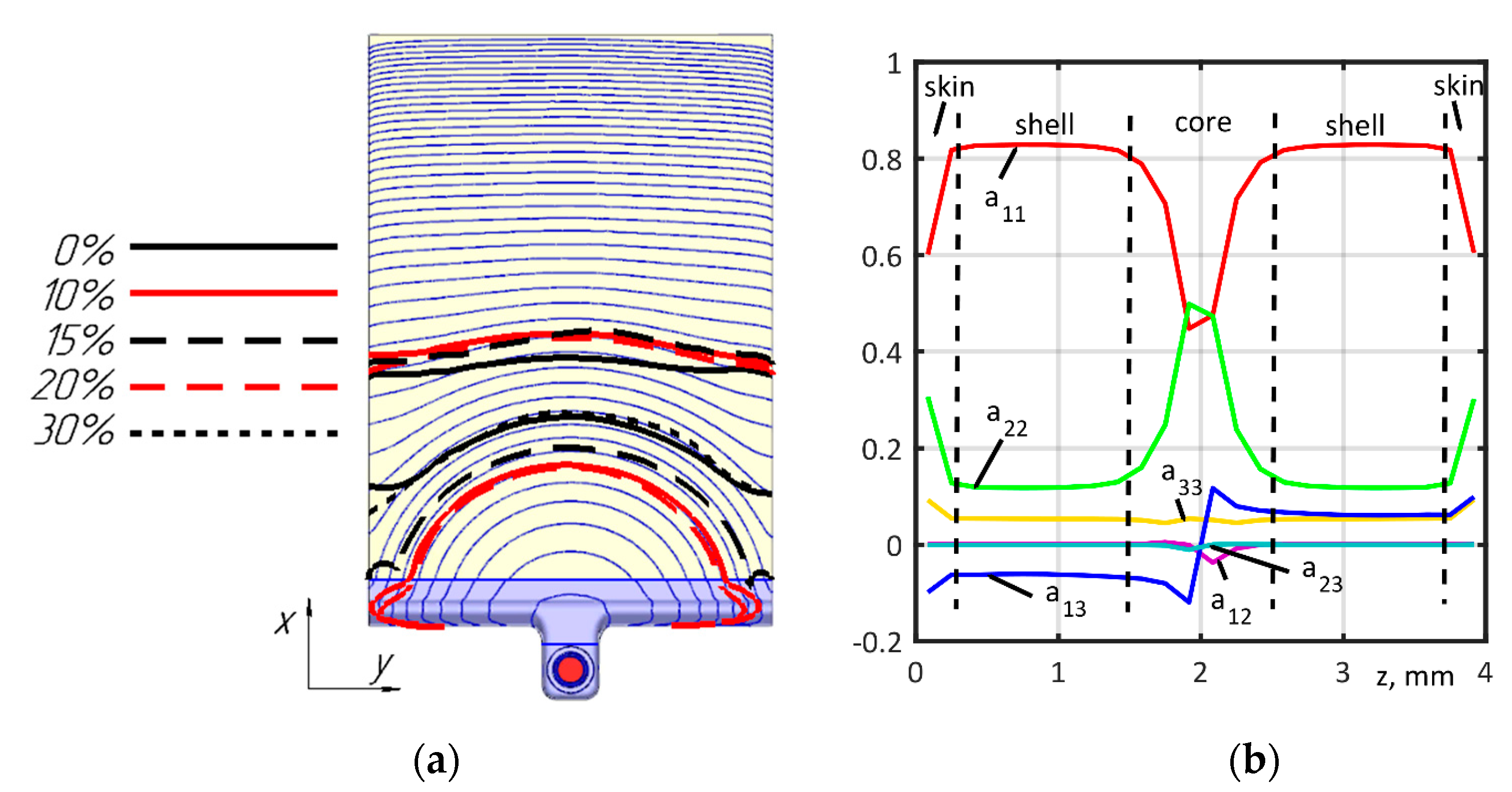
Figure 8.
Comparison of simulated and experimental filling: (a) Melt front, blue lines—calculated isolines at each 2% of filling time, black and red lines—experimentally obtained melt fronts; (b) Orientation tensor components, solid lines—calculated values, dash lines—mean experimentally obtained zones sizes.
Figure 9.
The microstructure of short-fiber reinforced PA6 with 30% carbon-fiber mass fraction along the following orientations: (a) 0°; (b) 90°.
Figure 9.
The microstructure of short-fiber reinforced PA6 with 30% carbon-fiber mass fraction along the following orientations: (a) 0°; (b) 90°.
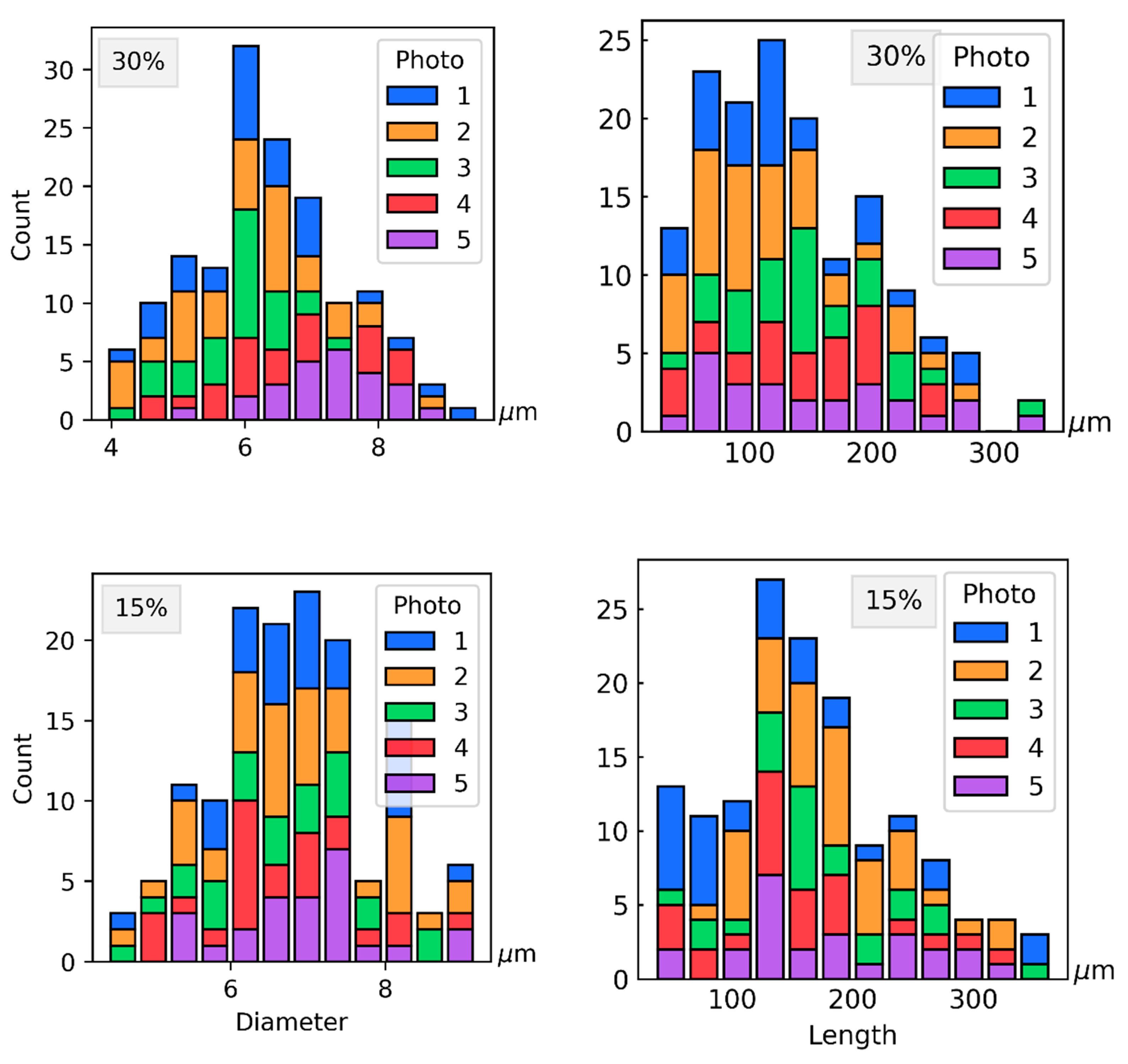
Figure 10.
Distribution of diameter and length in 30% and 15% fiber mass fraction samples.
Figure 10.
Distribution of diameter and length in 30% and 15% fiber mass fraction samples.
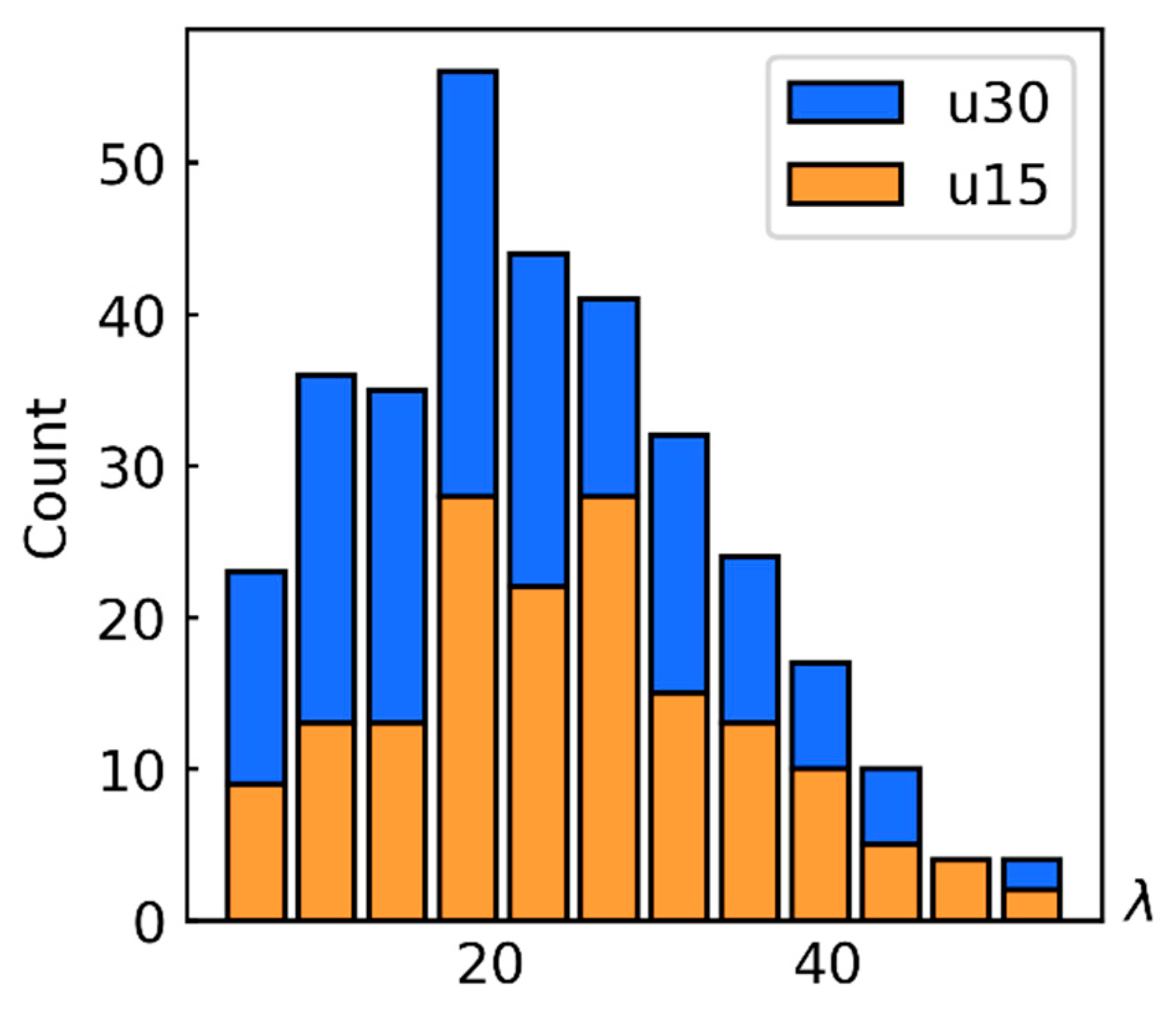
Figure 11.
Measured fiber aspect ratio distribution for 15% (u15) and 30% (u30) fiber mass fractions.
Figure 11.
Measured fiber aspect ratio distribution for 15% (u15) and 30% (u30) fiber mass fractions.
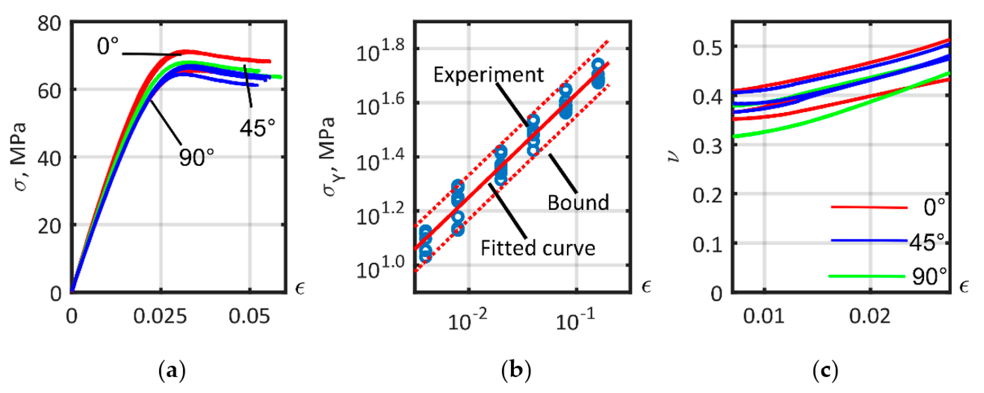
Figure 12.
Tensile test of ISO 527-2 PA6 matrix samples: (a) Tension curves; (b) Yield stress; (c) Poisson’s ratio.
Figure 12.
Tensile test of ISO 527-2 PA6 matrix samples: (a) Tension curves; (b) Yield stress; (c) Poisson’s ratio.
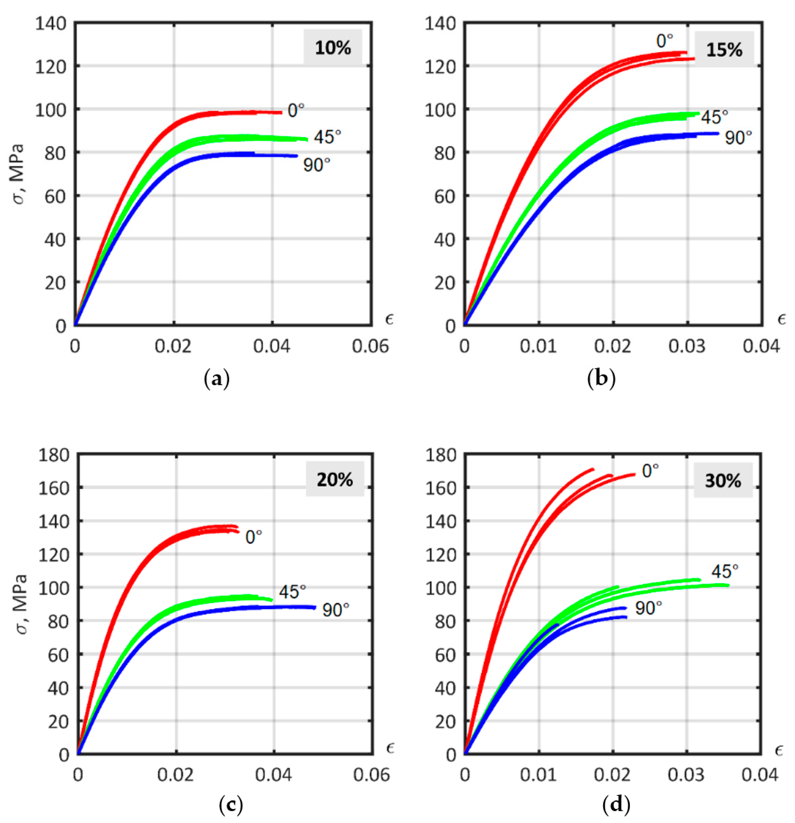
Figure 13.
Experimental stress–strain curves for ISO 527-2 samples of PA6 composites with different fiber mass fractions, cut at 0°, 45° and 90° angles to flow direction: (a) 10%; (b) 15%; (c) 20%; (d) 30%.
Figure 13.
Experimental stress–strain curves for ISO 527-2 samples of PA6 composites with different fiber mass fractions, cut at 0°, 45° and 90° angles to flow direction: (a) 10%; (b) 15%; (c) 20%; (d) 30%.
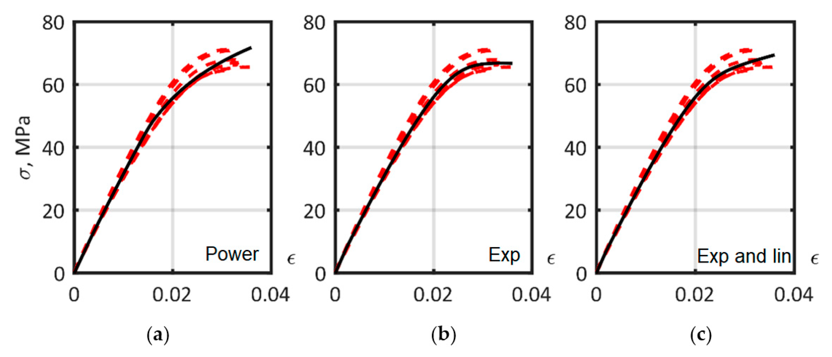
Figure 14.
The approximation of PA6 matrix ISO 527-2 tension curves, dashed lines—experiment, solid lines—model, with hardening laws: (a) power; (b) exponential; (c) exponential and linear. The solid lines show the optimized curves. Dashed lines are the experimental data.
Figure 14.
The approximation of PA6 matrix ISO 527-2 tension curves, dashed lines—experiment, solid lines—model, with hardening laws: (a) power; (b) exponential; (c) exponential and linear. The solid lines show the optimized curves. Dashed lines are the experimental data.
Figure 15.
Stress–strain curves of short-fiber reinforced PA6 with 30% carbon fiber were modeled using the exponential law. Comparison between: (a) Single AR value and AR distribution; (b) Single layer and multilayer analysis.
Figure 15.
Stress–strain curves of short-fiber reinforced PA6 with 30% carbon fiber were modeled using the exponential law. Comparison between: (a) Single AR value and AR distribution; (b) Single layer and multilayer analysis.
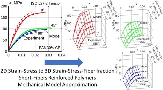
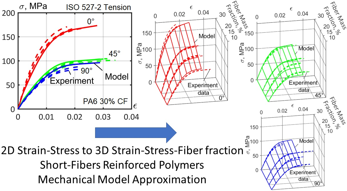
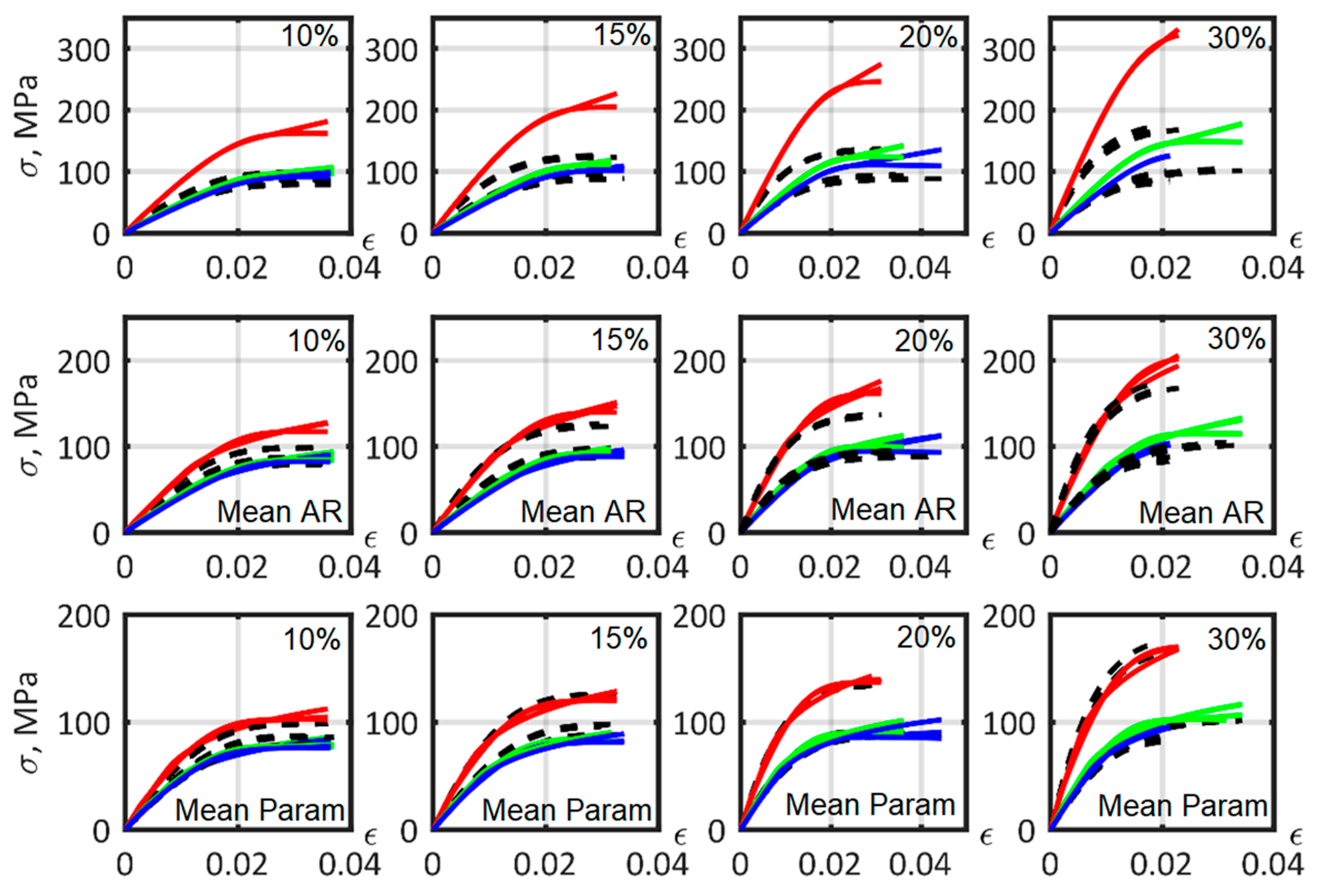
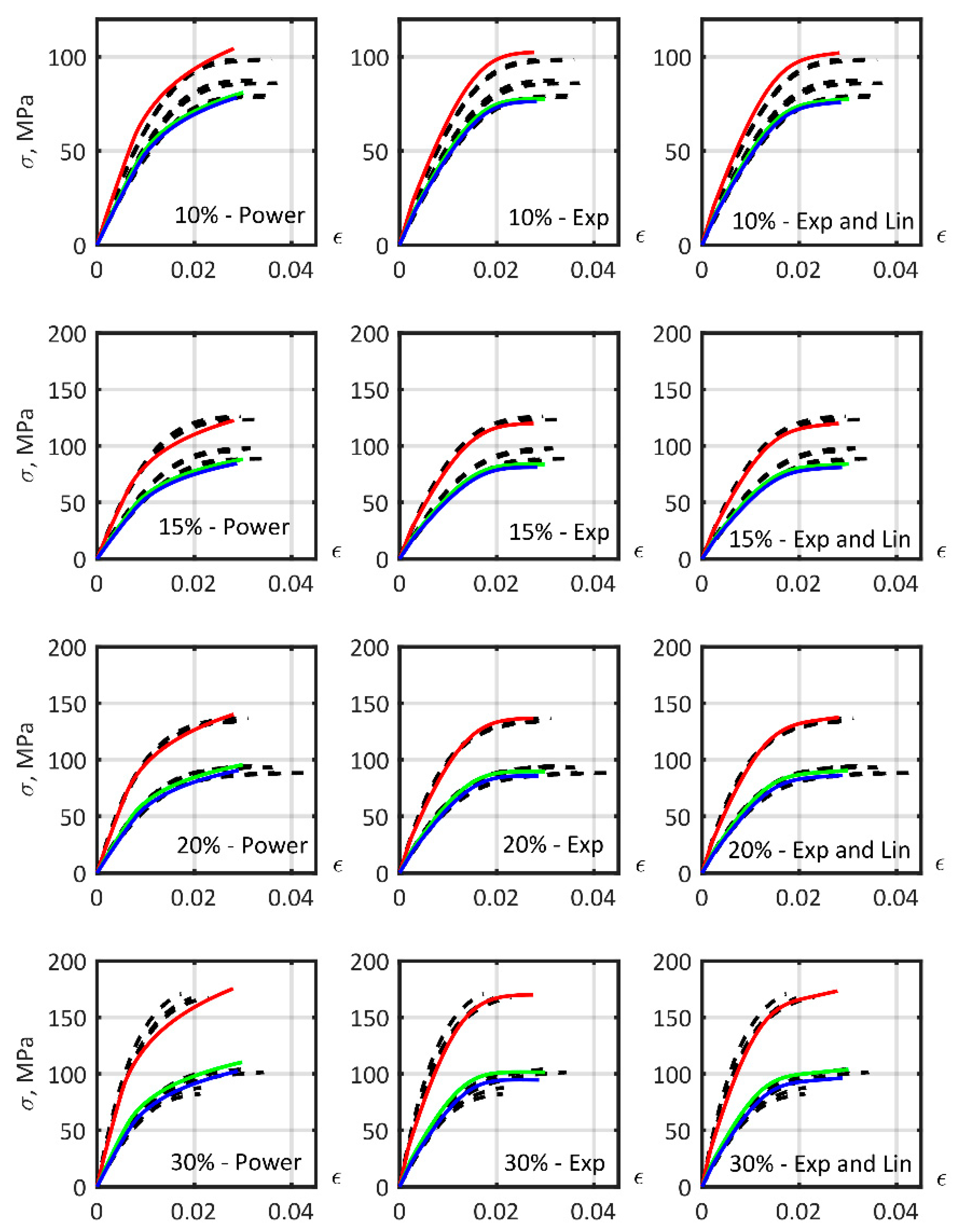
Figure 16.
Stress–strain curves for the model material for PA6 with different short carbon fiber mass fractions, orientated in different directions. From left to right: 10%, 15%, 20%, and 30% fiber mass fraction. From top to bottom: non-calibrated parameters; calibrated fiber aspect ratio; all matrix parameters and fiber aspect ratio calibrated. Material model—color lines: 0°—red lines, 45°—green lines, 90°—blue lines. Experimental data—black dashed lines.
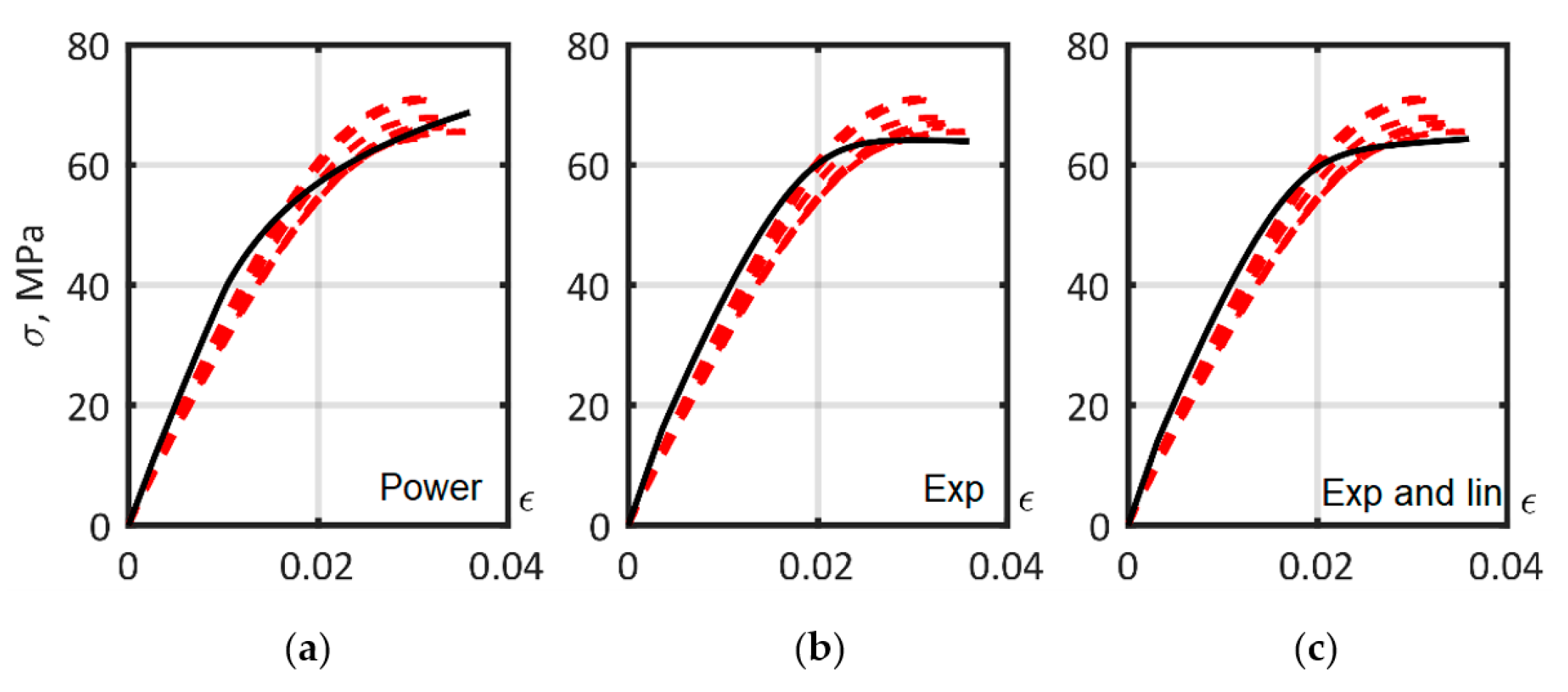
Figure 17.
Matrix models (solid lines) after the composite stiffness calibration with different hardening laws: (a) power; (b) exponential; (c) exponential and linear. Dashed lines—experiment.
Figure 17.
Matrix models (solid lines) after the composite stiffness calibration with different hardening laws: (a) power; (b) exponential; (c) exponential and linear. Dashed lines—experiment.
Figure 18.
Stress–strain curves prepared from the mean obtained strain limits, and using Tsai–Hill 3D transversely isotropic strain-based values for 10%, 15%, 20%, and 30% fiber mass fractions. Material model—color lines: 0°—red lines, 45°—green lines, 90°—blue lines. Experimental data—black dashed lines.
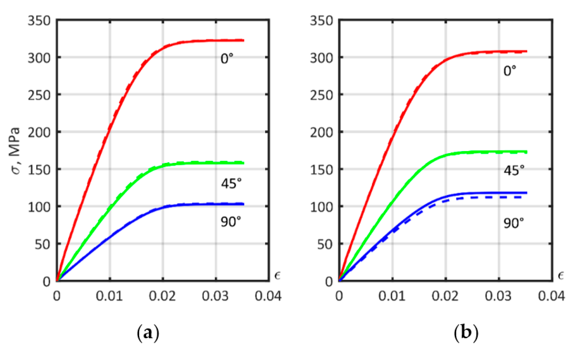
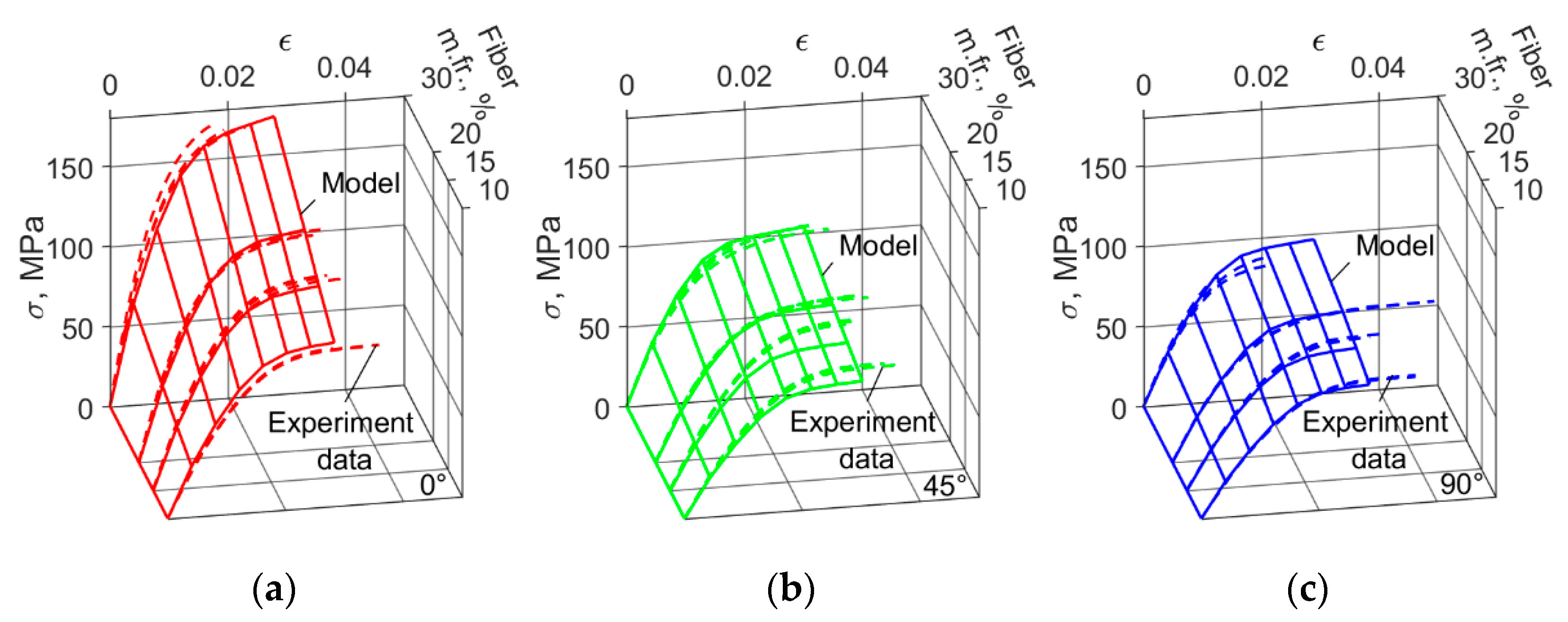
Figure 19.
Common mass fraction composite material models for all fibers. Exponent and linear hardening law case. For angles between the flow and load directions: (a) 0°; (b) 45°; (c) 90°.
Figure 19.
Common mass fraction composite material models for all fibers. Exponent and linear hardening law case. For angles between the flow and load directions: (a) 0°; (b) 45°; (c) 90°.
Table 1.
Calculated fiber orientation tensor components.
Table 1.
Calculated fiber orientation tensor components.
| Layer | Thickness, mm | a11 | a22 | a33 | a12 | a13 | a23 |
|---|
| 1 | 0.1667 | 0.603 | 0.304 | 0.0929 | 0.00104 | 0.00019 | 0.00011 |
| 2 | 1.5003 | 0.821 | 0.126 | 0.0533 | 0.00087 | 0.00001 | 0.00003 |
| 3 | 0.1667 | 0.711 | 0.244 | 0.0451 | −0.00131 | −0.00033 | 0.00008 |
| 4 | 0.3334 | 0.461 | 0.486 | 0.0526 | −0.01870 | −0.00113 | −0.00495 |
| 5 | 0.1667 | 0.711 | 0.244 | 0.0451 | −0.00131 | −0.00033 | 0.00008 |
| 6 | 1.5003 | 0.821 | 0.126 | 0.0533 | 0.00087 | 0.00001 | 0.00003 |
| 7 | 0.1667 | 0.603 | 0.304 | 0.0929 | 0.00104 | 0.00019 | 0.00011 |
Table 2.
Calibrated pure PA6 tension curve parameters of elastoplastic matrix material models.
Table 2.
Calibrated pure PA6 tension curve parameters of elastoplastic matrix material models.
| Hardening Law | Power | Exponential | Exponential and Linear |
|---|
| Young’s modulus, MPa | 3341 | 3547 | 3552 |
| Yield stress, MPa | 12.57 | 8.27 | 6.68 |
| Hardening modulus, MPa | - | 60.59 | 55.41 |
| Hardening Exponent m | 0.21891 | 433.69 | 528.67 |
| Linear hardening modulus k, MPa | 158.12 | - | 623.17 |
| Relative error, % | 5.32 | 4.81 | 4.77 |
Table 3.
Fiber aspect ratio (AR) calibration for composites with different fiber mass fraction.
Table 3.
Fiber aspect ratio (AR) calibration for composites with different fiber mass fraction.
| Hardening Law | Fiber Mass Fraction, % | Mean AR Model | Param. CV, % |
|---|
| 10 | 15 | 20 | 30 |
|---|
| | Aspect ratio |
|---|
| Power | 14.00 | 16.53 | 14.47 | 14.82 | 15.00 | 7.35 |
| Exponential | 14.53 | 16.94 | 15.14 | 15.47 | 15.52 | 6.60 |
| Exponential and linear | 14.30 | 16.75 | 14.71 | 15.27 | 15.30 | 7.03 |
Table 4.
Calibration of all parameters of the matrix elastoplasticity model and fiber aspect ratio.
Table 4.
Calibration of all parameters of the matrix elastoplasticity model and fiber aspect ratio.
| Parameter | Fiber Mass Fraction, % | Mean Parameters Model | Parameters CV, % |
|---|
| 10 | 15 | 20 | 30 |
|---|
| Power Law |
| Young’s modulus, MPa | 4383 | 4437 | 4162 | 3759 | 4185 | 7.4 |
| Yield stress, MPa | 12.3 | 12.6 | 10.2 | 9.9 | 11.2 | 12.3 |
| Hardening modulus, MPa | 147.6 | 161.9 | 124.6 | 137.0 | 142.8 | 11.1 |
| Hardening exponent | 0.1995 | 0.2238 | 0.2023 | 0.2475 | 0.2183 | 10.2 |
| Fibers’ AR | 8.84 | 12.23 | 14.19 | 16.79 | 13.01 | 25.8 |
| Exponential Law |
| Young’s modulus, MPa | 4654 | 4615 | 4741 | 3994 | 4501 | 7.6 |
| Yield stress, MPa | 13.8 | 21.2 | 12.4 | 16.1 | 15.9 | 24.3 |
| Hardening modulus, MPa | 59.2 | 51.0 | 51.5 | 38.7 | 50.1 | 17.0 |
| Hardening exponent | 404.8 | 370.6 | 353.6 | 377.8 | 376.7 | 5.7 |
| Fibers’ AR | 9.02 | 12.25 | 13.37 | 16.62 | 12.8 | 24.4 |
| Exponential and linear law |
| Young’s modulus, MPa | 4672 | 4842 | 4625 | 3994 | 4533 | 8.2 |
| Yield stress, MPa | 13.6 | 13.0 | 14.5 | 14.5 | 13.9 | 5.4 |
| Hardening modulus, MPa | 56.6 | 54.9 | 46.1 | 37.0 | 48.6 | 18.6 |
| Hardening exponent | 447.1 | 417.7 | 381.1 | 458.3 | 426.0 | 8.1 |
| Hardening linear modulus, MPa | 208.8 | 216.0 | 144.1 | 188.4 | 189.3 | 17.1 |
| Fibers’ AR | 8.82 | 12.36 | 13.80 | 16.54 | 12.9 | 24.9 |
Table 5.
Mean relative error of stress–strain curve prediction of different fiber mass fraction composites with models based on fibers and matrix characteristics obtained experimentally, mean fiber aspect ratio calibrated models, and the mean parameter model.
Table 5.
Mean relative error of stress–strain curve prediction of different fiber mass fraction composites with models based on fibers and matrix characteristics obtained experimentally, mean fiber aspect ratio calibrated models, and the mean parameter model.
| Hardening Law | Fiber Mass Fraction, % | Mean Level of Error, % |
|---|
| 10 | 15 | 20 | 30 |
|---|
| Models, based on fibers and matrix characteristics obtained experimentally |
| Power | 29.0 | 25.7 | 35.8 | 35.9 | 31.6 |
| Exponential | 27.8 | 25.2 | 33.7 | 34.7 | 30.4 |
| Exponential and linear | 28.6 | 25.9 | 36.1 | 35.7 | 31.6 |
| Mean fiber aspect ratio calibrated models |
| Power | 11.7 | 12.1 | 12.0 | 11.1 | 11.7 |
| Exponential | 11.5 | 12.3 | 11.3 | 11.7 | 11.7 |
| Exponential and linear | 11.7 | 12.5 | 12.6 | 12.2 | 12.3 |
| Mean with the calibration of all matrix and fiber aspect ratio parameters |
| Power | 7.4 | 7.6 | 4.9 | 7.7 | 6.9 |
| Exponential | 6.9 | 6.8 | 4.1 | 8.0 | 6.5 |
| Exponential and linear | 7.0 | 6.9 | 3.9 | 7.9 | 6.4 |
Table 6.
Failure criteria strain limits for different fiber mass fraction cases.
Table 6.
Failure criteria strain limits for different fiber mass fraction cases.
| Parameters | Fiber Mass Fraction, % | Mean Strain Limits | Parameters CV, % |
|---|
| 10 | 15 | 20 | 30 |
|---|
| Power law |
| Axial tensile strain limit, 10−2 | 2.009 | 2.957 | 1.944 | 1.880 | 2.197 | 23.16 |
| Inplane tensile strain limit, 10−2 | 3.516 | 3.855 | 3.573 | 2.151 | 3.274 | 23.30 |
| Transverse shear strain limit, 10−2 | 5.606 | 5.140 | 5.235 | 4.364 | 5.086 | 10.26 |
| Exponential law |
| Axial tensile strain limit, 10−2 | 1.566 | 2.353 | 1.832 | 2.031 | 1.945 | 17.05 |
| Inplane tensile strain limit, 10−2 | 2.999 | 3.524 | 3.430 | 2.278 | 3.058 | 18.57 |
| Transverse shear strain limit, 10−2 | 5.873 | 5.249 | 5.355 | 4.076 | 5.138 | 14.77 |
| Exponential and linear law |
| Axial tensile strain limit, 10−2 | 2.141 | 2.402 | 1.908 | 1.944 | 2.099 | 10.81 |
| Inplane tensile strain limit, 10−2 | 3.684 | 3.573 | 3.559 | 2.012 | 3.207 | 24.90 |
| Transverse shear strain limit, 10−2 | 5.607 | 5.140 | 5.140 | 4.798 | 5.171 | 6.42 |
Table 7.
Mean relative error (%) of ultimate strain prediction for different fiber mass fraction composites with models based on fiber and matrix characteristics obtained experimentally, mean fiber aspect ratio calibrated models, and the mean parameter model.
Table 7.
Mean relative error (%) of ultimate strain prediction for different fiber mass fraction composites with models based on fiber and matrix characteristics obtained experimentally, mean fiber aspect ratio calibrated models, and the mean parameter model.
| Hardening Law | Fiber Mass Fraction, % | Mean Level of Error, % |
|---|
| 10 | 15 | 20 | 30 |
|---|
| Power | 16.24 | 7.79 | 18.92 | 56.63 | 24.90 |
| Exponential | 17.30 | 8.87 | 19.73 | 55.04 | 25.24 |
| Exponential and linear | 16.26 | 7.79 | 19.02 | 56.36 | 24.86 |


