
Linearization of Composite Material Damage Model Results and Its Impact on the Subsequent Stress–Strain Analysis


Abstract
:1. Introduction
2. Methodology
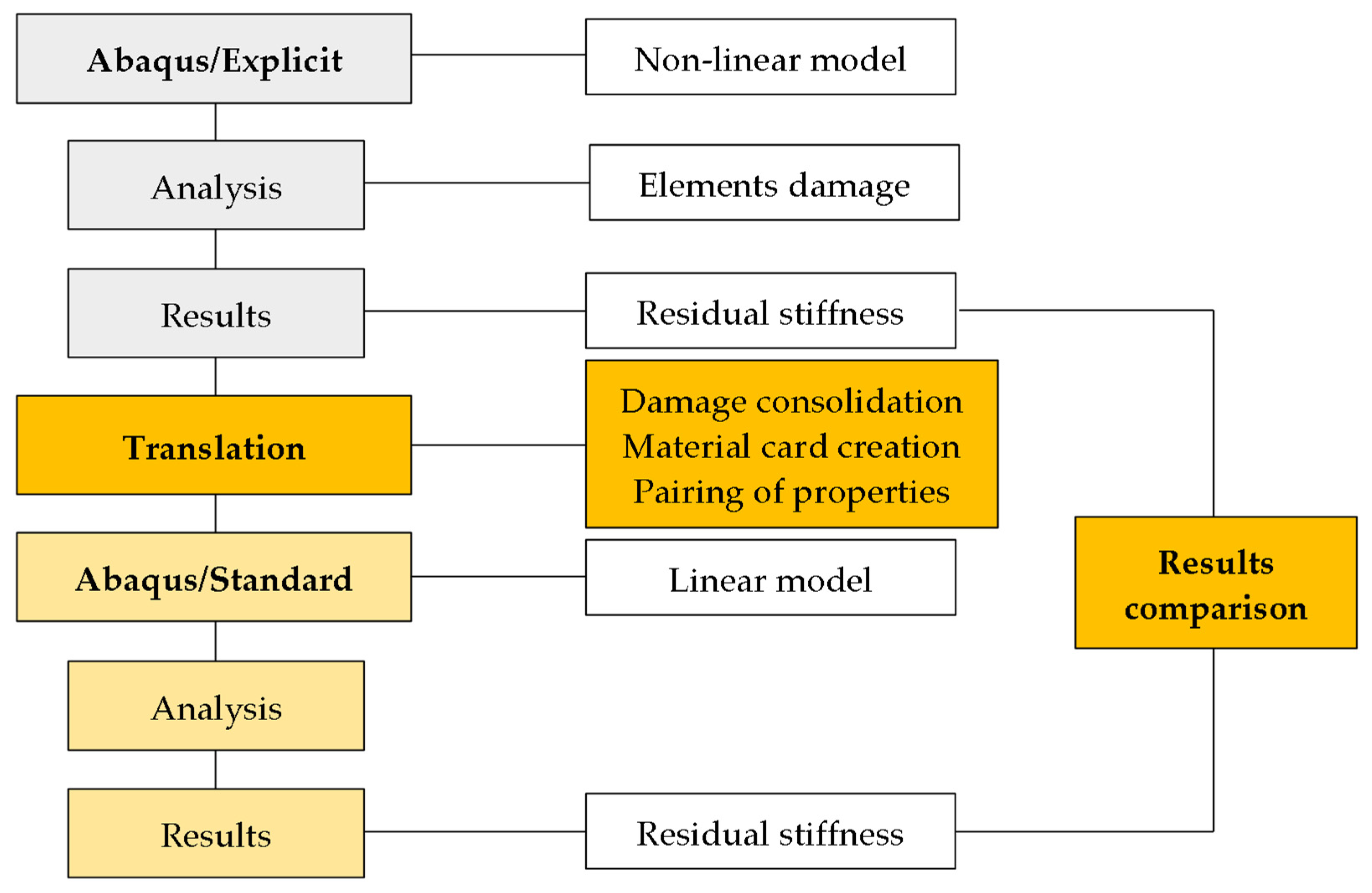
2.1. Workflow Overview
2.2. Basic Calculus
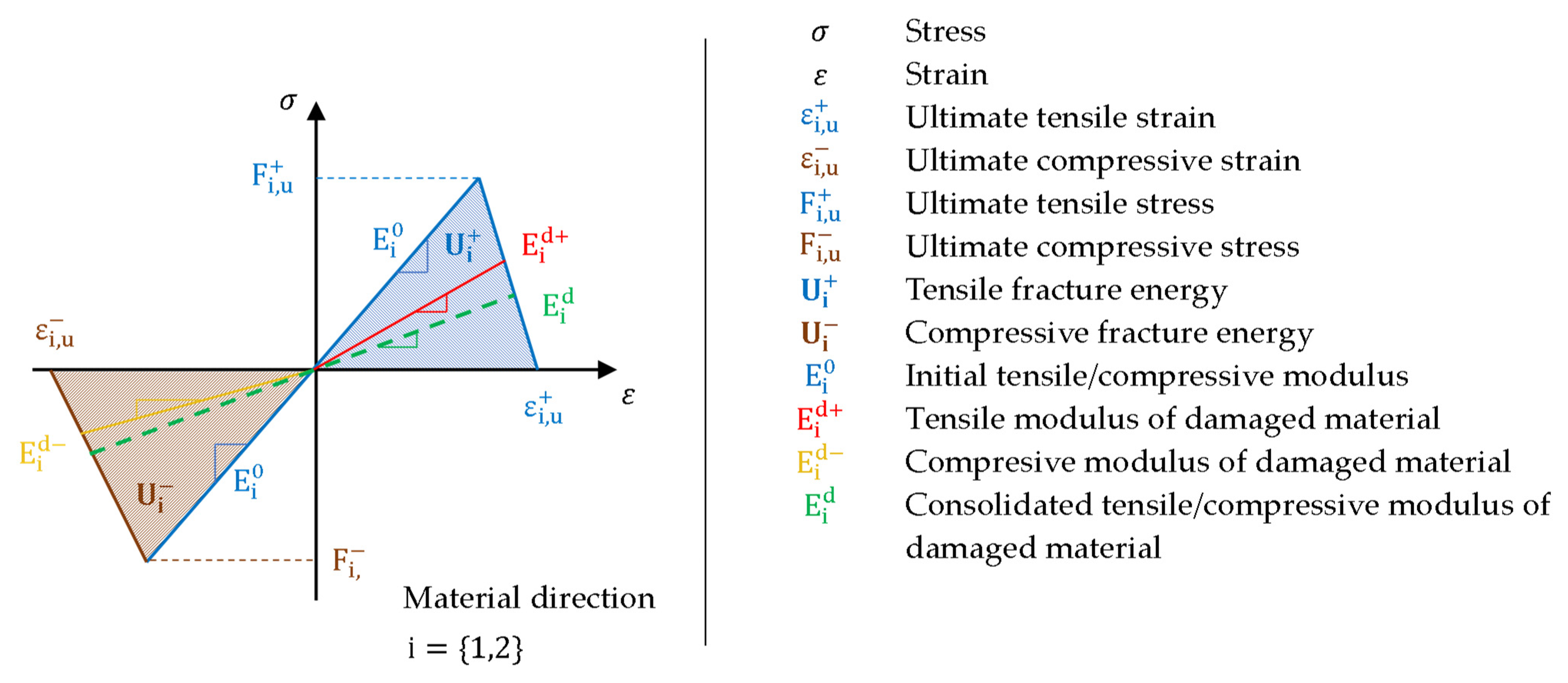
2.3. Graphic Interpretation of Hashin’s Violation
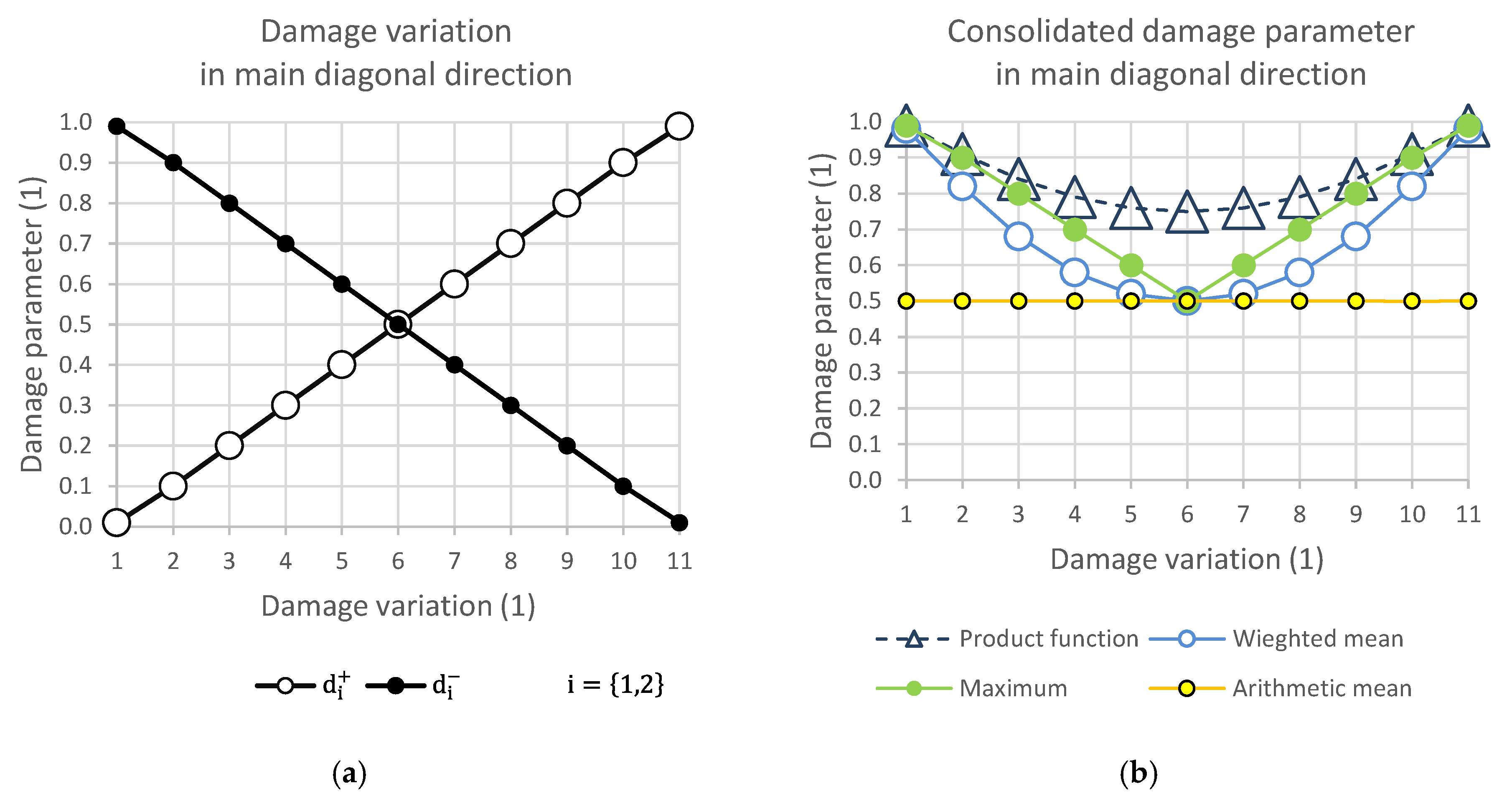
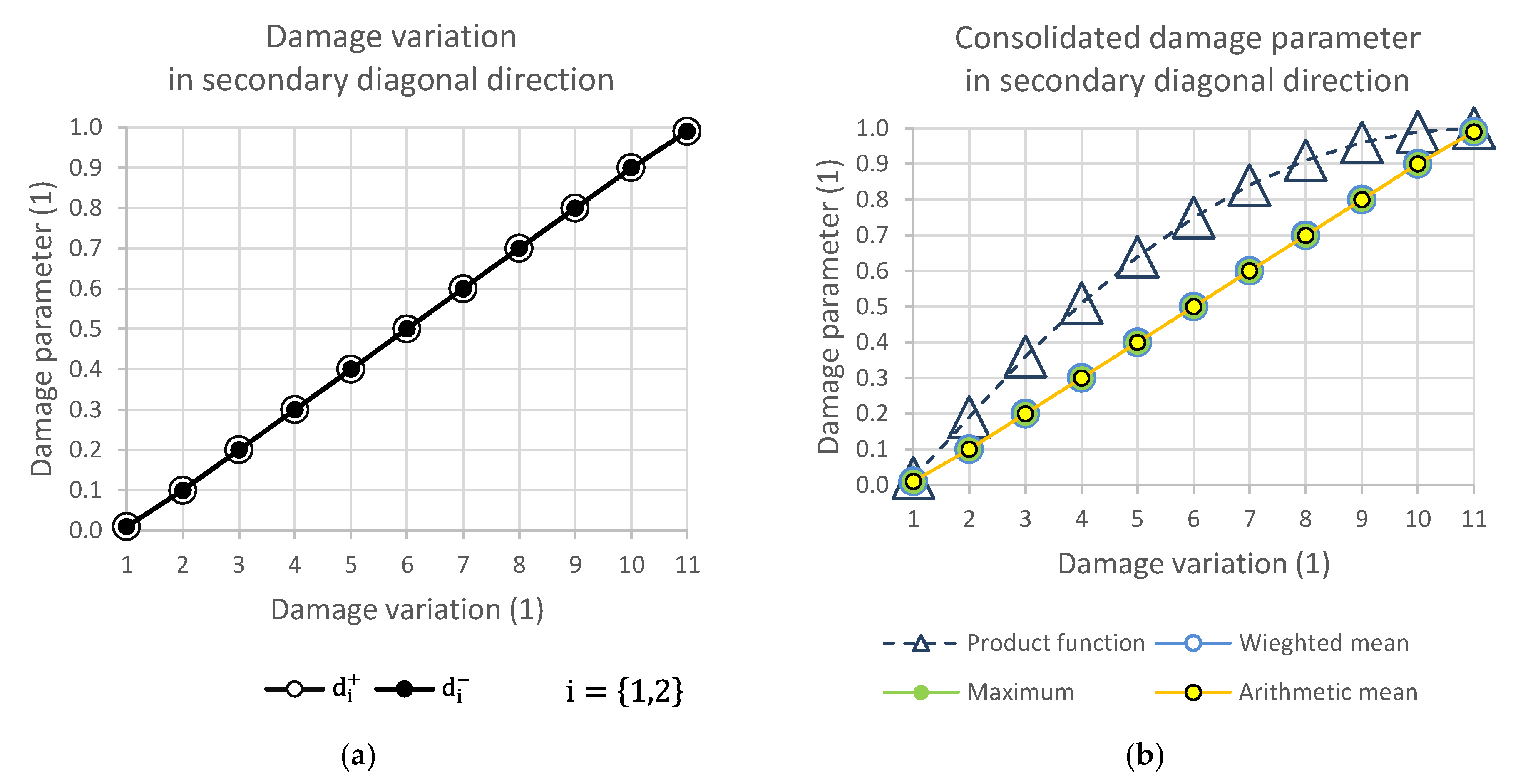
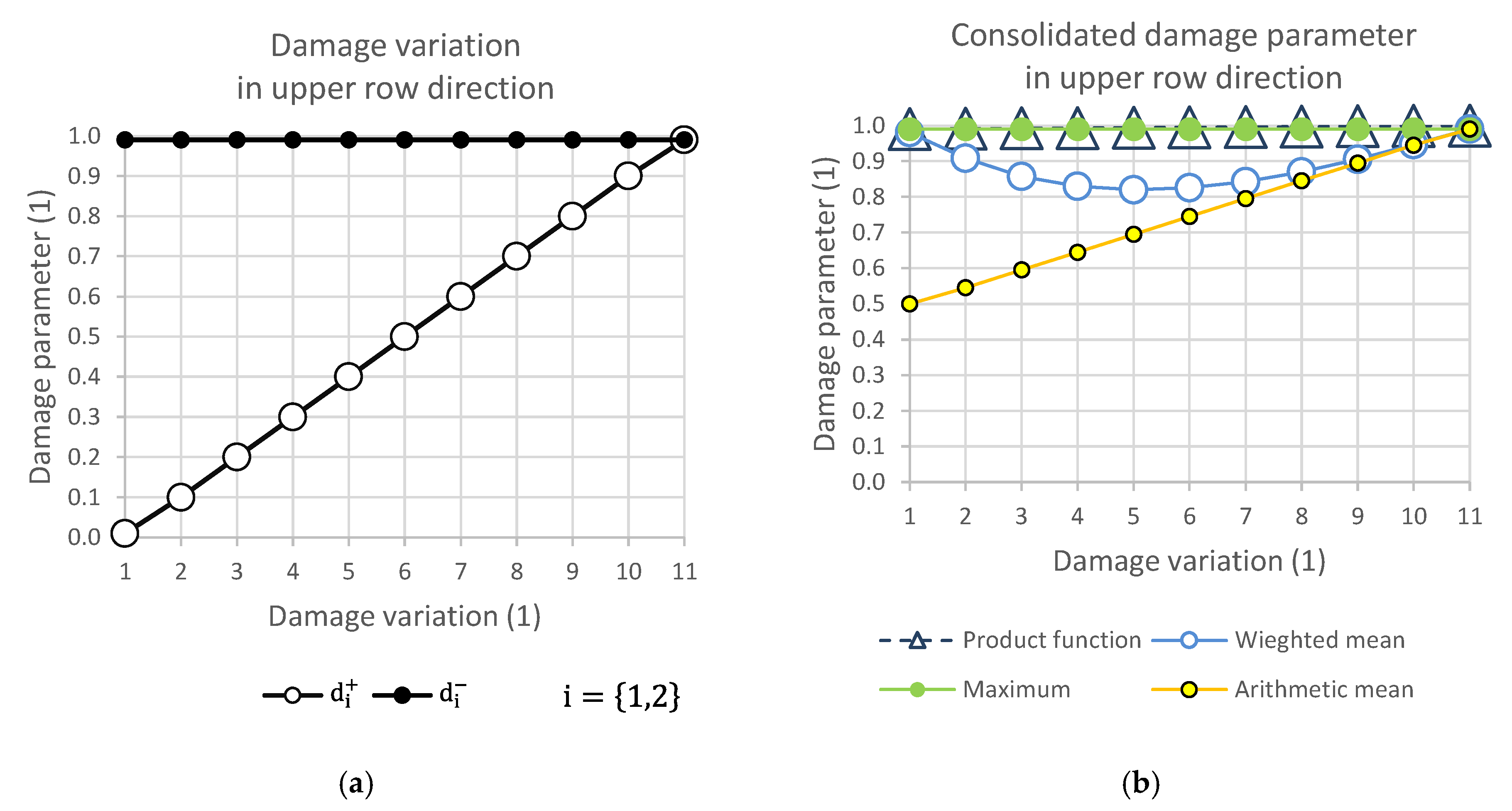
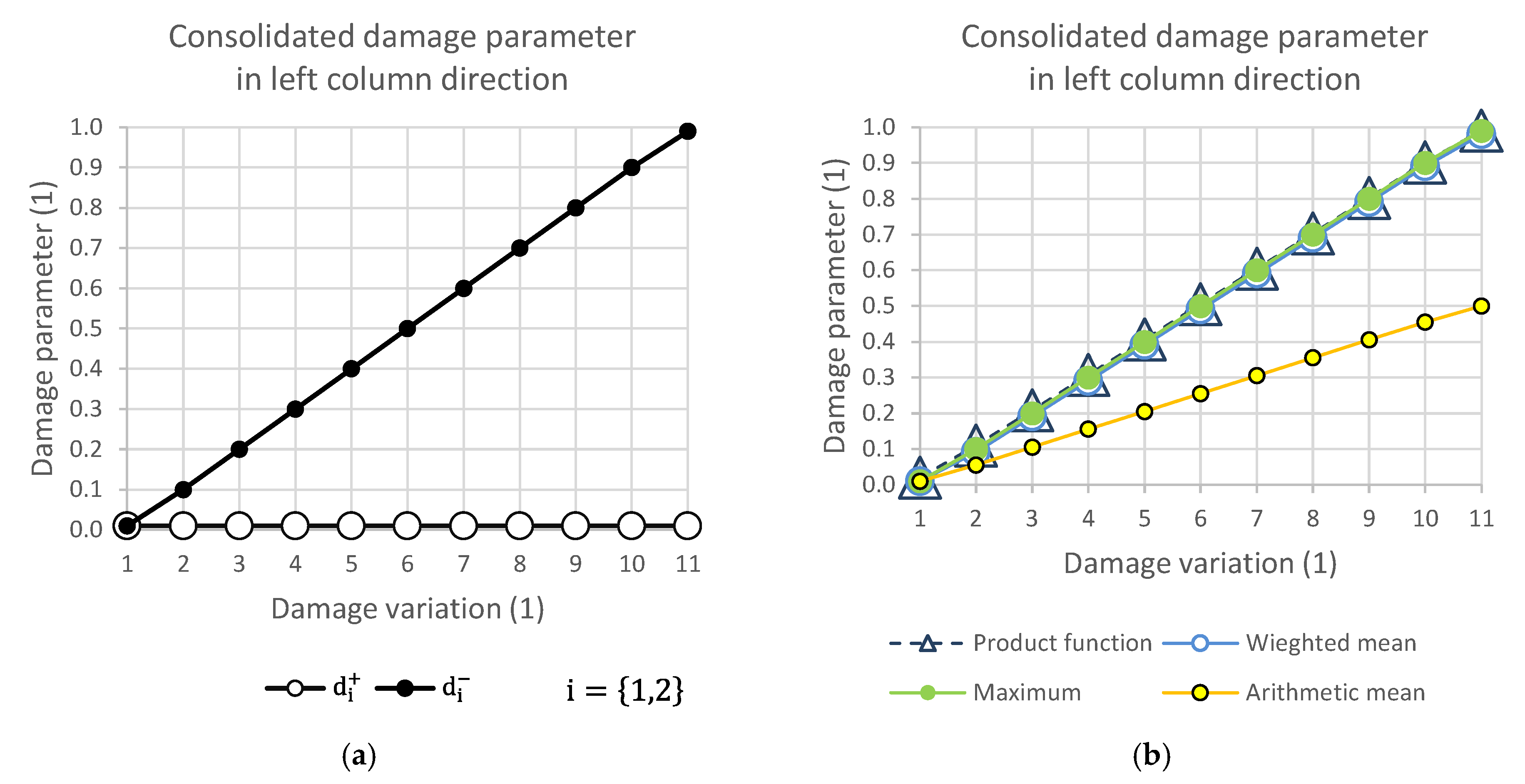
2.4. Consolidation Function
2.5. Material Card Generation
2.6. Material Properties
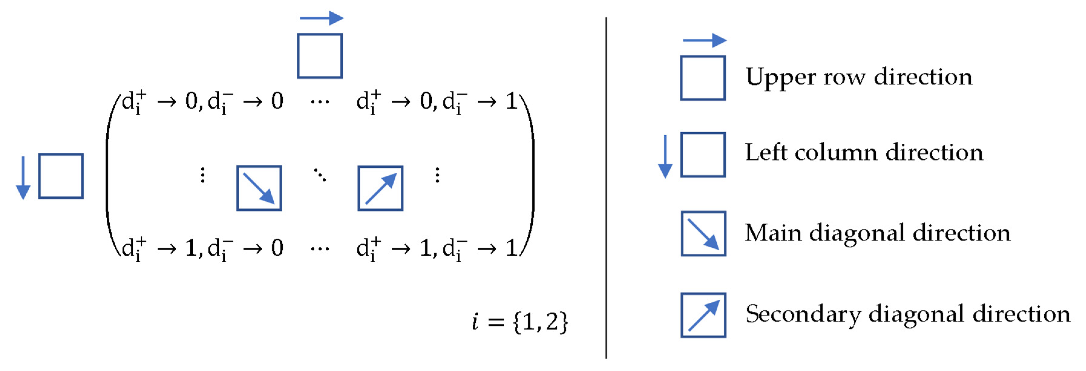
2.7. Damage Variation Matrix and Response of Consolidation Functions
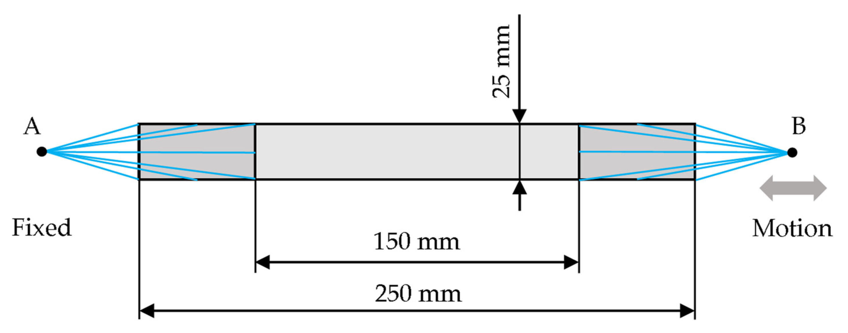
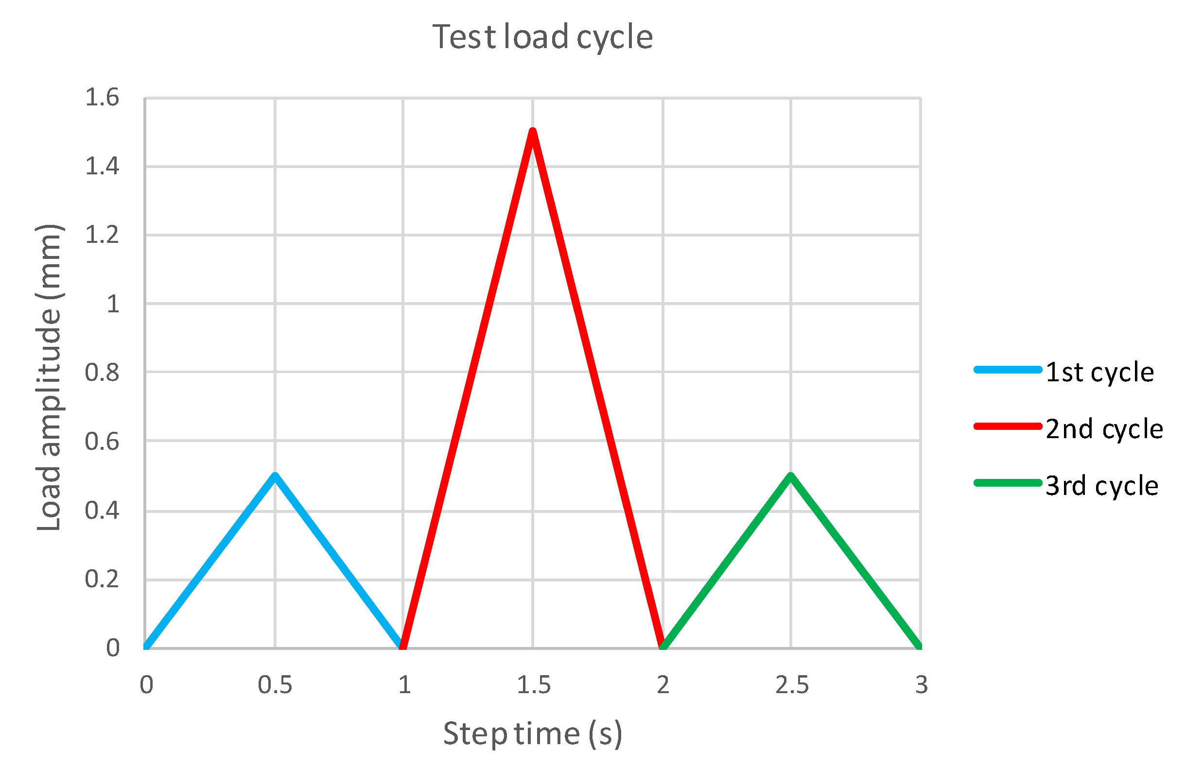
2.8. Testing Examples
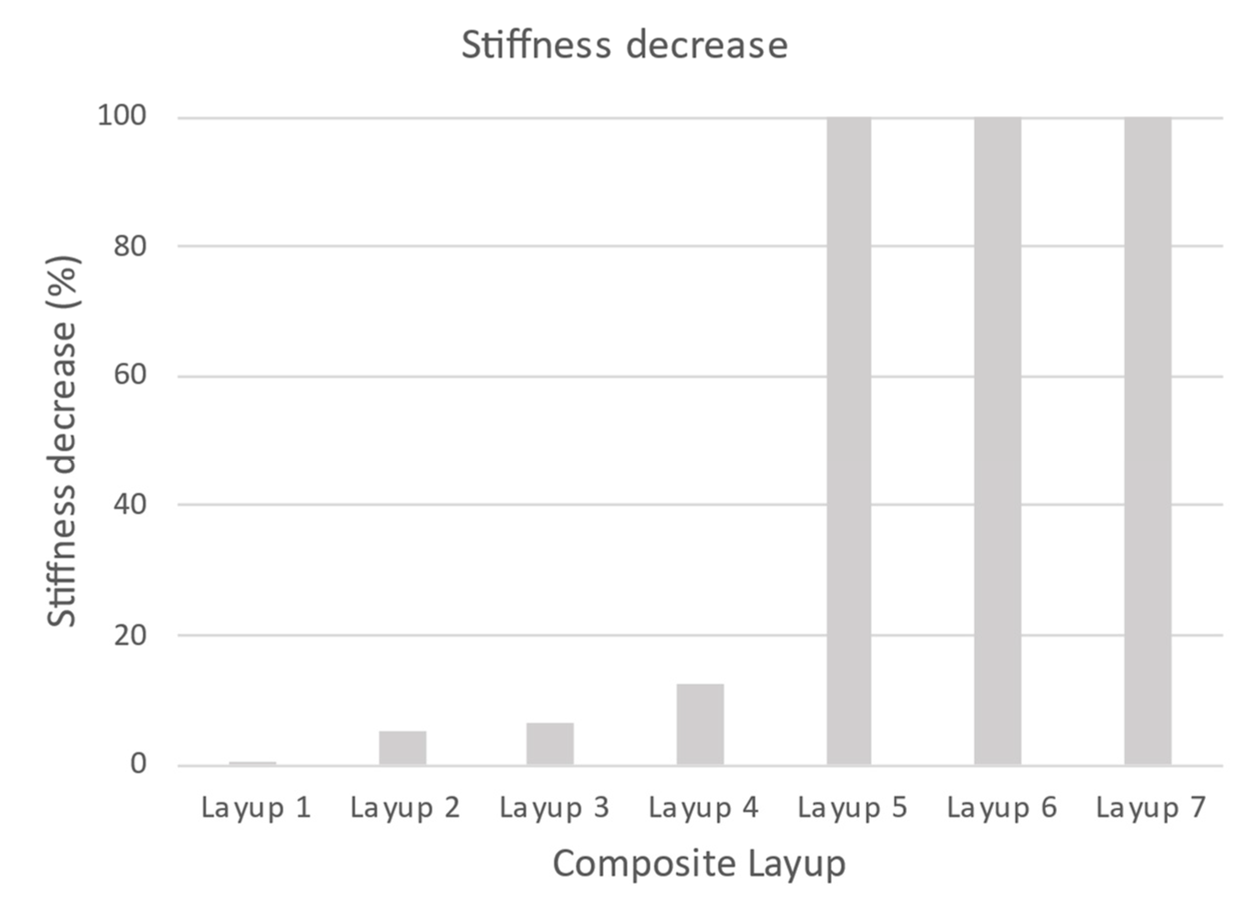
3. Results and Discussion
4. Conclusions
Author Contributions
Funding
Institutional Review Board Statement
Informed Consent Statement
Data Availability Statement
Conflicts of Interest
Abbreviations
| (MPa) | Undamaged material stress response tensor | |
| (MPa) | Effective stress tensor | |
| (MPa) | General stress tensor | |
| (1) | General strain tensor | |
| (MPa) | Elastic modulus of non-damaged material in the direction 1 | |
| (MPa) | Elastic modulus of non-damaged material in the direction 2 | |
| (MPa) | Shear modulus of non-damaged material in plane 12 | |
| (MPa) | Transverse shear modulus of non-damaged material in plane 13 | |
| (MPa) | Transverse shear modulus of non-damaged material in plane 23 | |
| (1) | Poisson’s ratio of undamaged material in plane 12 | |
| (MPa) | Consolidated elastic modulus of damaged material in the direction 1 | |
| (MPa) | Consolidated elastic of damaged material in the direction 2 | |
| (MPa) | Consolidated shear modulus of damaged material in plane 12 | |
| (MPa) | Consolidated transverse shear modulus of damaged material in plane 13 | |
| (MPa) | Consolidated transverse shear modulus of damaged material in plane 23 | |
| (1) | Poisson’s ratio of undamaged material in plane 12 | |
| (MPa) | Tensile elastic modulus of damaged material in the direction 1 | |
| (MPa) | Compressive elastic of damaged material in the direction 1 | |
| (MPa) | Tensile elastic modulus of damaged material in the direction 2 | |
| (MPa) | Compressive elastic of damaged material in the direction 2 | |
| (1) | Consolidated damage factor in the direction 1 | |
| (1) | Consolidated damage factor in the direction 2 | |
| (1) | Consolidated damage factor in plane 12 | |
| (1) | Consolidated shear damage factor | |
| (1) | Tensile damage factor in the direction 1 | |
| (1) | Compressive damage factor in the direction 1 | |
| (1) | Tensile damage factor in the direction 2 | |
| (1) | Compressive damage factor in the direction 2 | |
| (MPa) | Stiffness matrix of undamaged material | |
| (MPa−1) | Compliance matrix of undamaged material | |
| (MPa) | Stiffness matrix of damaged material | |
| (MPa−1) | Compliance matrix of damaged material | |
| (1) | Damage operator matrix | |
| (MPa) | Ultimate tensile stress in direction 1 | |
| (MPa) | Ultimate compressive stress in direction 1 | |
| (MPa) | Ultimate tensile stress in direction 2 | |
| (MPa) | Ultimate compressive stress in direction 2 | |
| (MPa) | Ultimate shear stress in plane 12 | |
| (MPa) | Ultimate shear stress in plane 13 | |
| (MPa) | Ultimate shear stress in plane 23 | |
| (1) | Ultimate tensile strain in direction 1 | |
| (1) | Ultimate compressive strain in direction 1 | |
| (1) | Ultimate tensile strain in direction 2 | |
| (1) | Ultimate compressive strain in direction 2 | |
| (mJ/mm2) | Tensile fracture energy in direction 1 | |
| (mJ/mm2) | Compressive fracture energy in direction 1 | |
| (mJ/mm2) | Tensile fracture energy in direction 2 | |
| (mJ/mm2) | Compressive fracture energy in direction 2 | |
| Consolidation damage function in direction 1 | ||
| Consolidation damage function in direction 2 | ||
| Consolidation damage function in plane 12 |
References
- ABAQUS-6.14. Theory Manual. Available online: http://130.149.89.49:2080/v6.14/ (accessed on 8 December 2021).
- Lahey, S.R.; Miller, P.M.; Reymond, M. MSC.NASTRAN 2004 Reference Manual; Version 68; MSC.Software Corporation: Santa Ana, CA, USA, 2004; Volume 2, pp. 583–584. [Google Scholar]
- Bathe, K. Finite Element Procedures; PHI Learning Private Limited: Delhi, India, 1996; Volume 1. [Google Scholar]
- Matzenmiller, A.; Lubliner, J.; Taylor, R. A constitutive model for anisotropic damage in fiber-composites. Mech. Mater. 1995, 20, 125–152. [Google Scholar] [CrossRef]
- Donghyun, Y.; Sangdeok, K.; Jaehoon, K.; Youngdae, D. Development and Evaluation of Crack Band Model Implemented Progressive Failure Analysis Method for Notched Composite Laminate. Appl. Sci. 2019, 9, 5572. [Google Scholar] [CrossRef] [Green Version]
- Koloor, S.; Karimzadeh, A.; Yidris, N.; Petru, M.; Ayatollahi, M.; Tamin, M. An Energy-Based Concept for Yielding of Multidirectional FRP Composite Structures Using a Mesoscale Lamina Damage Model. Polymers 2020, 12, 157. [Google Scholar] [CrossRef] [PubMed] [Green Version]
- Koloor, S.; Karimzadeh, A.; Abdulah, M.; Petru, M.; Yidris, N.; Sapuan, S.; Tamin, M. Linear-Nonlinear Stiffness Responses of carbon Fiber-Reinforced Polymer Composite Materials and Structures. Polymers 2021, 13, 344. [Google Scholar] [CrossRef] [PubMed]
- Murakami, S. Continuum Damage Mechanics: A Continuum Mechanics Approach to the Analysis of Damage and Fracture; Springer Science & Business Media: Berlin/Heidelberg, Germany, 2012; Volume 185. [Google Scholar]
- Wei, L.; Zhu, W.; Yu, Z.; Liu, J.; Wei, X. A new three-dimensional progressive damage model for fiber-reinforced polymer laminates and its applications to large open-hole panels. Compos. Sci. Technol. 2019, 182, 107757. [Google Scholar] [CrossRef]
- Liao, B.; Jia, L.; Zhou, J.; Lei, H.; Gao, R.; Lin, Y.; Fang, D. An explicit–implicit combined model for predicting residual strength of composite cylinders subjected to low velocity impact. Compos. Struct. 2020, 247, 112450. [Google Scholar] [CrossRef]
- Jia, L.; Yu, L.; Zhang, K.; Li, M.; Jia, Y.; Blackman, B.; Dear, J. Combined modelling and experimental studies of failure in thick laminates under out-of-plane shear. Compos. Part B Eng. 2016, 105, 8–22. [Google Scholar] [CrossRef]
- Kim, E.; Rim, M.; Lee, I.; Hwang, T. Composite damage model based on continuum damage mechanics and low velocity impact analysis of composite plates. Compos. Struct. 2013, 95, 123–134. [Google Scholar] [CrossRef]
- Šedek, J.; Bělský, P. Numerical evaluation of barely visible impact damage in a carbon fibre-reinforced composite panel with shear loading. WIT Trans. Eng. Sci. 2017, 116, 73–85. [Google Scholar]
- Vlach, J.; Raška, J.; Horňas, J.; Petrusová, L. Impacted area description effect on strength of laminate determined by calculation. Procedia Struct. Integr. 2022, 35, 132–140. [Google Scholar] [CrossRef]
- Afshar, A.; Daneshyar, A.; Mohammadi, S. XFEM analysis of fiber bridging in mixed-mode crack propagation in composites. Compos. Struct. 2015, 125, 314–327. [Google Scholar] [CrossRef]
- Hashin, Z. Failure criteria for unidirectional fiber composites. J. Appl. Mech. 1980, 47, 329–334. [Google Scholar] [CrossRef]
- Hashin, Z.; Rotem, A. A fatigue failure criterion for fiber-reinforced materials. J. Compos. Mater. 1973, 7, 448–464. [Google Scholar] [CrossRef] [Green Version]
- Berthelot, J.M. Matériaux Composites, Comportement Mécanique et Analyse Des Structures, 1st ed.; Masson: Paris, France, 1992; pp. 154–196. [Google Scholar]
- Daniel, I.M.; Ishai, O. Engineering Mechanics of Composite Materials, 2nd ed.; Oxford University Press: New York, NY, USA, 2006; pp. 268–272. [Google Scholar]
- ASTM D3039/D3039M-14; Standard Test Method for Tensile Properties of Polymer Matrix Composite Materials. ASTM International: Philadelphia, PA, USA, 2014.


| Function | Consolidate Parameter | Consolidate Variable |
|---|---|---|
| Method | Consolidate Condition | |
|---|---|---|
| Arithmetic mean | ||
| Weighted mean | ||
| Maximum | ||
| Product function | ||
| Shear function | ||
| Plane Stress | Shear-Bending Coupling |
|---|---|
| (MPa) | (MPa) | (1) | (1) | (MPa) |
| (MPa) | (MPa) | (1) | (MPa) | (MPa) | (MPa) |
| 129,840 | 13,340 | 0.26 | 4890 | 4890 | 4630 |
| (MPa) | (MPa) | (MPa) | (MPa) | (MPa) | (MPa) |
| 2965.41 | 2911.81 | 100.88 | 109.42 | 100.76 | 98.41 |
| (mJ/mm2) | (mJ/mm2) | (mJ/mm2) | (mJ/mm2) |
| 35.56 | 34.28 | 0.92 | 1.08 |
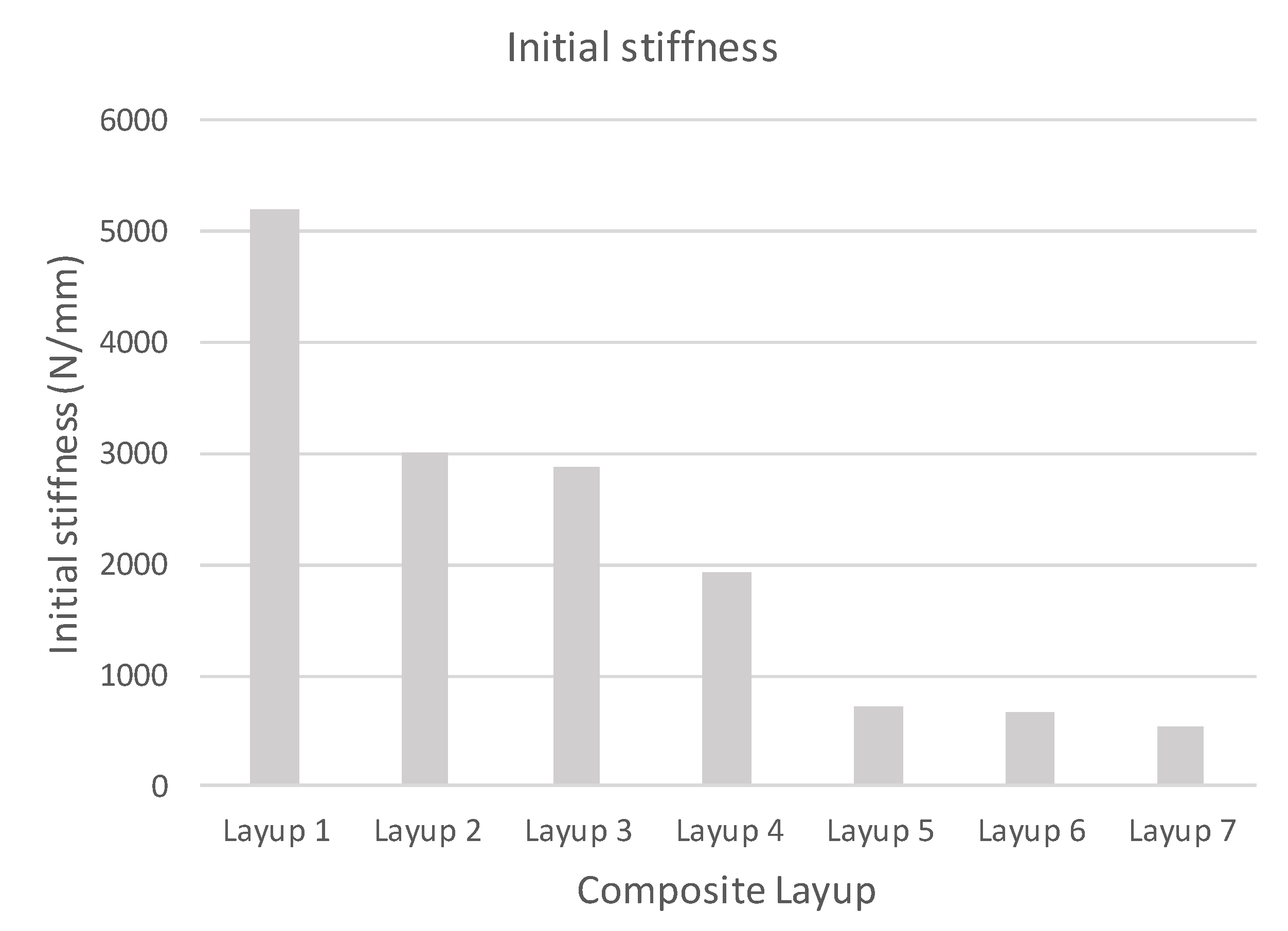
| Layup Id. | Layup Design | Layup Id. | Layup Design |
|---|---|---|---|
| 1 | [0°/0°/0°/0°] | 5 | [45°/−45°/−45°/45°] |
| 2 | [0°/+45°/−45°/0°] | 6 | [45°/90°/90°/45°] |
| 3 | [0°/90°/90°/0°] | 7 | [90°/90°/90°/90°] |
| 4 | [0°/+45°/−45°/90°] |
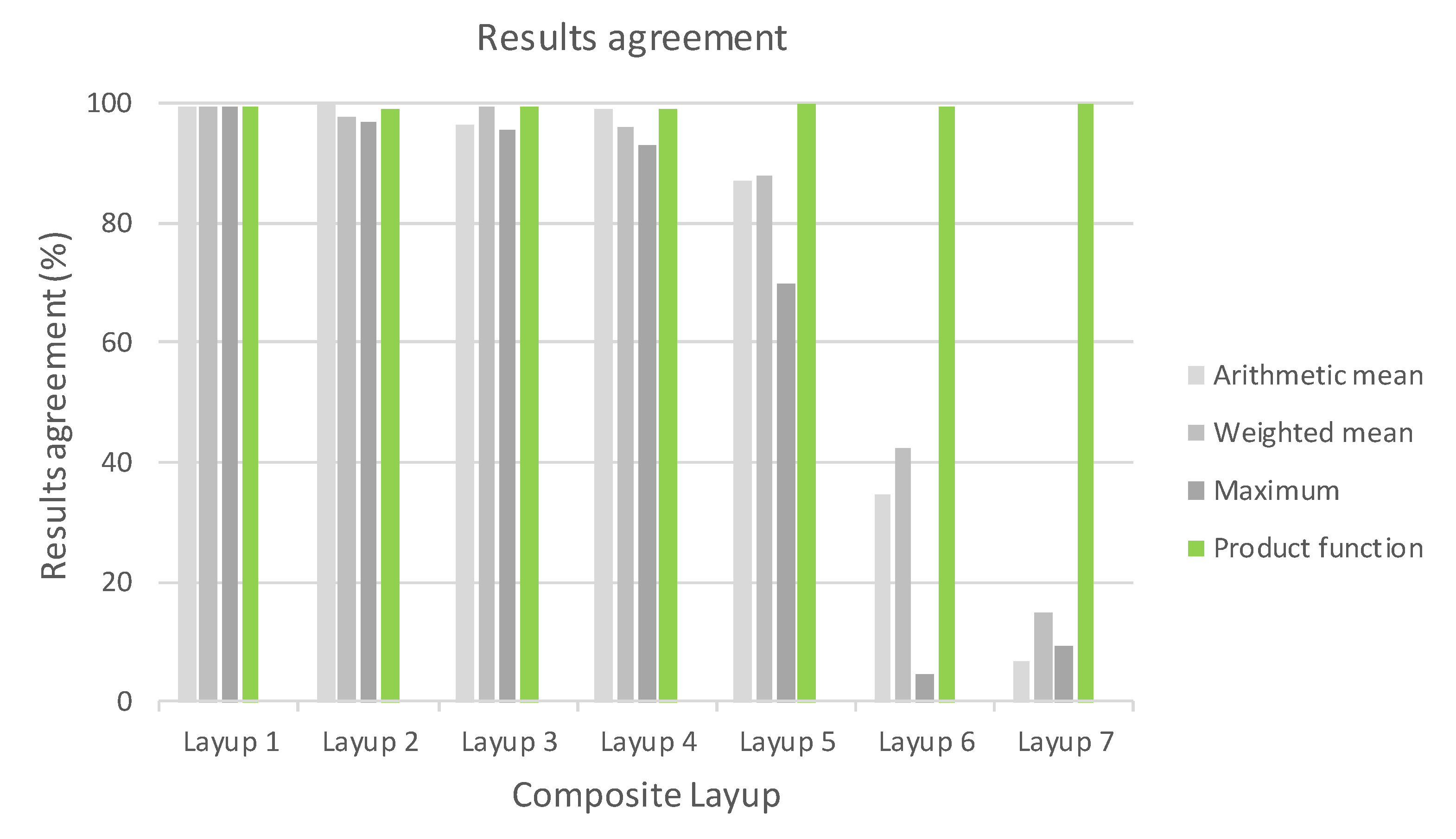
| Consolidate Function | Layup 1 | Layup 2 | Layup 3 | Layup 4 | Layup 5 | Layup 6 | Layup 7 |
|---|---|---|---|---|---|---|---|
| [−] | [%] | [%] | [%] | [%] | [%] | [%] | [%] |
| Arithmetic mean | 0.38 | 0.03 | 3.75 | 0.81 | 12.94 | 65.19 | 93.05 |
| Weighted mean | 0.38 | 2.17 | 0.58 | 4.09 | 12.03 | 57.44 | 85.23 |
| Maximum | 0.38 | 3.24 | 4.51 | 6.98 | 30.23 | 95.41 | 90.50 |
| Product function | 0.38 | 1.05 | 0.66 | 1.06 | 0.02 | 0.50 | 0.08 |
Publisher’s Note: MDPI stays neutral with regard to jurisdictional claims in published maps and institutional affiliations. |
© 2022 by the authors. Licensee MDPI, Basel, Switzerland. This article is an open access article distributed under the terms and conditions of the Creative Commons Attribution (CC BY) license (https://creativecommons.org/licenses/by/4.0/).
Share and Cite
Vlach, J.; Doubrava, R.; Růžek, R.; Raška, J.; Horňas, J.; Kadlec, M. Linearization of Composite Material Damage Model Results and Its Impact on the Subsequent Stress–Strain Analysis. Polymers 2022, 14, 1123. https://doi.org/10.3390/polym14061123
Vlach J, Doubrava R, Růžek R, Raška J, Horňas J, Kadlec M. Linearization of Composite Material Damage Model Results and Its Impact on the Subsequent Stress–Strain Analysis. Polymers. 2022; 14(6):1123. https://doi.org/10.3390/polym14061123
Chicago/Turabian StyleVlach, Jarmil, Radek Doubrava, Roman Růžek, Jan Raška, Jan Horňas, and Martin Kadlec. 2022. "Linearization of Composite Material Damage Model Results and Its Impact on the Subsequent Stress–Strain Analysis" Polymers 14, no. 6: 1123. https://doi.org/10.3390/polym14061123
APA StyleVlach, J., Doubrava, R., Růžek, R., Raška, J., Horňas, J., & Kadlec, M. (2022). Linearization of Composite Material Damage Model Results and Its Impact on the Subsequent Stress–Strain Analysis. Polymers, 14(6), 1123. https://doi.org/10.3390/polym14061123