
Modelling of Environmental Ageing of Polymers and Polymer Composites—Durability Prediction Methods

 , ,
, ,  ,
,  and
and 
Abstract
:1. Introduction
2. Models for Predicting Material Durability and Service Lifetime
2.1. Rate Models
2.1.1. Arrhenius Model
2.1.2. Eyring’s Model
2.1.3. Zhurkov’s Model
2.2. Superposition Principles
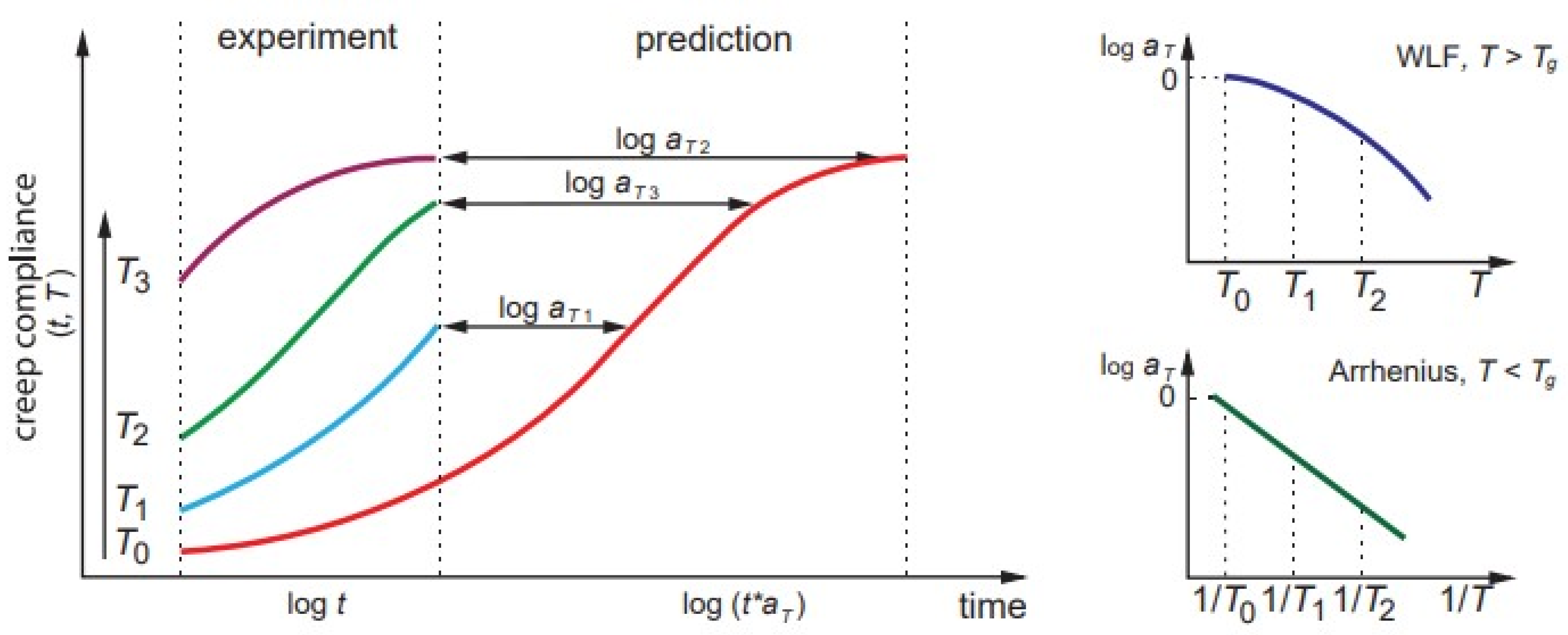
2.2.1. Time–Temperature Superposition Principle
2.2.2. Time–Moisture Superposition Principle
2.2.3. Time–Stress Superposition Principle
2.2.4. Time-Ageing Time Superposition
2.3. Plasticity-Controlled Failure
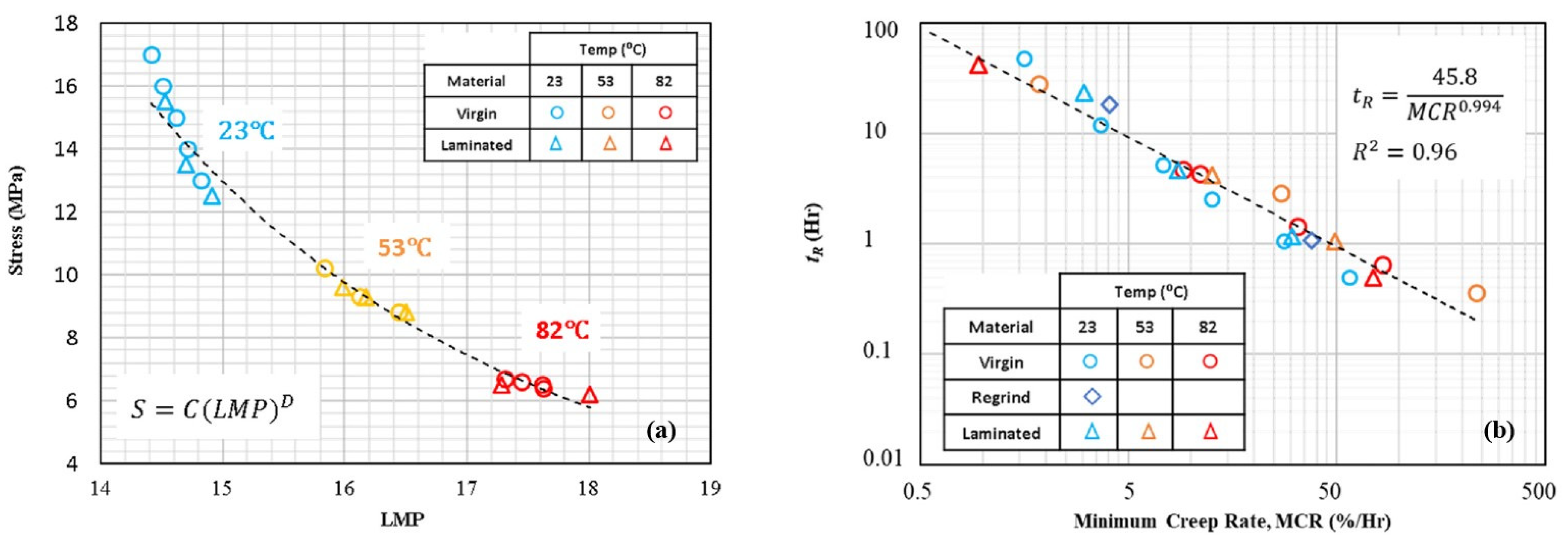
2.4. Parametric Methods for Creep
2.5. Fatigue Prediction Methods
2.5.1. Factors Affecting Fatigue Damage
- (i)
- Material related factors: fibre type and dimensions, matrix type, fibre volume content, reinforcement structure (unidirectional, multidirectional, woven, braided, spatially reinforced, etc.), laminate stacking sequence, etc.
- (ii)
- Testing related factors: loading conditions (stress ratio, cyclic frequency, monotonic/variable frequency, axial/multiaxial loading, force/displacement-controlled loading), and environmental conditions (temperature, humidity, water/salt water, UV).
- (iii)
- Manufacturing and storage-related factors: manufacturing process, inherent defects and voids, thermal or ageing pre-history, etc.
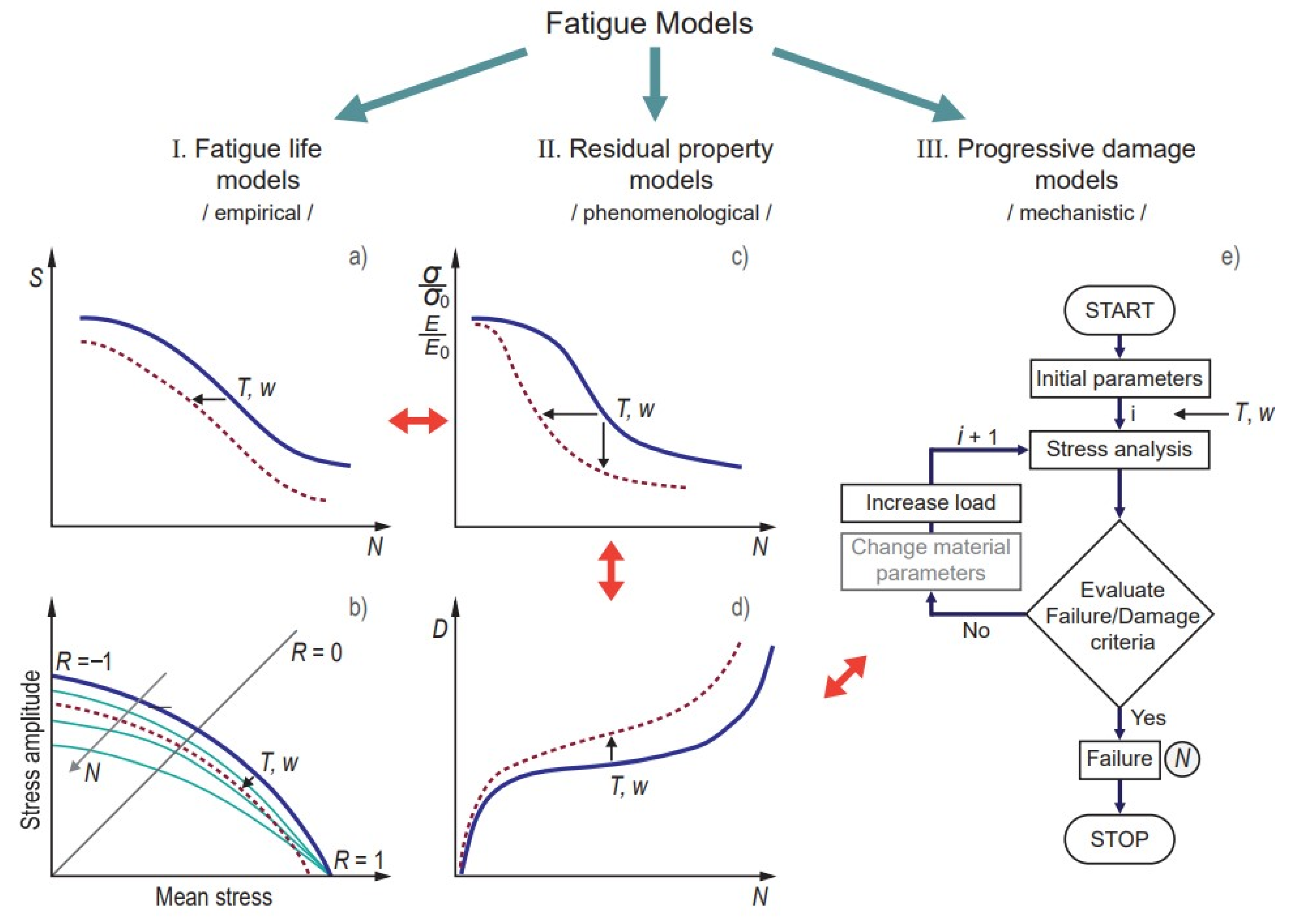
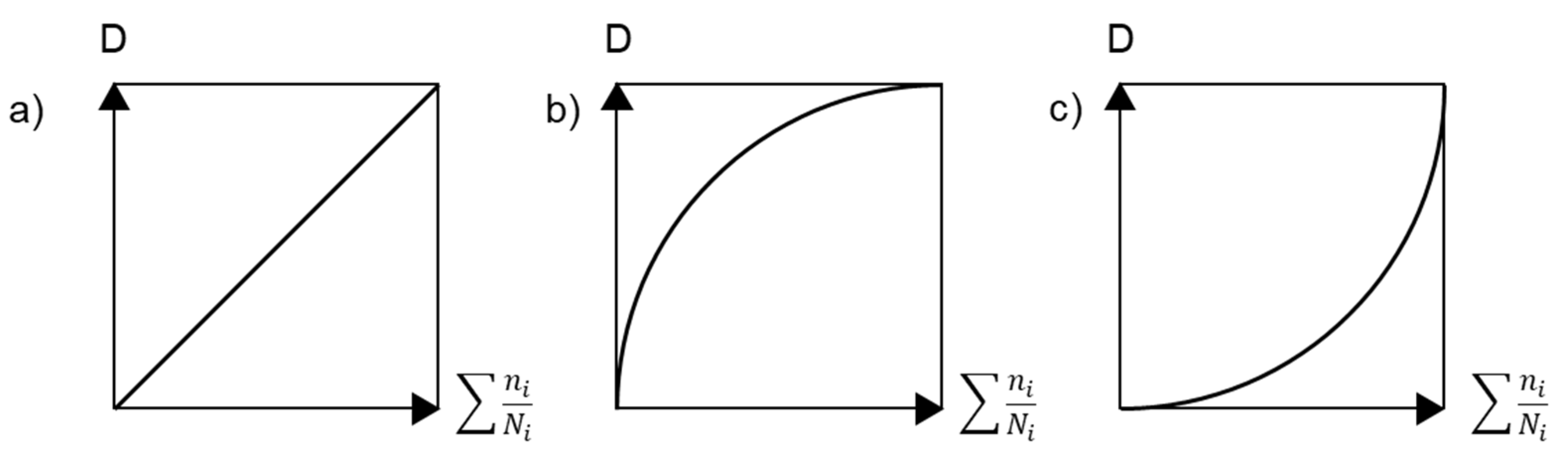
2.5.2. Classification of Fatigue Models
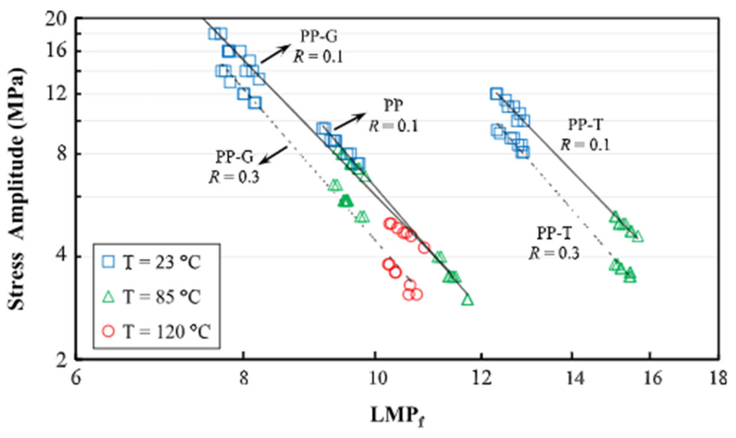
2.5.3. Fatigue Prediction under the Environmental Impact
3. Discussion
4. Conclusions
Author Contributions
Funding
Institutional Review Board Statement
Informed Consent Statement
Data Availability Statement
Acknowledgments
Conflicts of Interest
References
- Echtermeyer, A.T.; Gagani, A.; Krauklis, A.; Mazan, T. Multiscale Modelling of Environmental Degradation-First Steps. In Durability of Composites in a Marine Environment 2. Solid Mechanics and Its Applications; Davies, P., Rajapakse, Y., Eds.; Springer: Berlin/Heidelberg, Germany, 2018; Volume 245, pp. 135–149. [Google Scholar] [CrossRef]
- Frigione, M.; Rodríguez-Prieto, A. Can Accelerated Aging Procedures Predict the Long Term Behavior of Polymers Exposed to Different Environments? Polymers 2021, 13, 2688. [Google Scholar] [CrossRef] [PubMed]
- Gibhardt, D.; Doblies, A.; Meyer, L.; Fiedler, B. Effects of Hygrothermal Ageing on the Interphase, Fatigue, and Mechanical Properties of Glass Fibre Reinforced Epoxy. Fibers 2019, 7, 55. [Google Scholar] [CrossRef] [Green Version]
- Krauklis, A.E. Modular Paradigm for Composites: Modeling Hydrothermal Degradation of Glass Fibers. Fibers 2021, 9, 83. [Google Scholar] [CrossRef]
- Laycock, B.; Nikolić, M.; Colwell, J.M.; Gauthier, E.; Halley, P.; Bottle, S.; George, G. Lifetime prediction of biodegradable polymers. Prog. Polym. Sci. 2017, 71, 144–189. [Google Scholar] [CrossRef] [Green Version]
- Plota, A.; Masek, A. Lifetime Prediction Methods for Degradable Polymeric Materials—A Short Review. Materials 2020, 13, 4507. [Google Scholar] [CrossRef] [PubMed]
- Krauklis, A.E.; Karl, C.W.; Rocha, I.B.C.M.; Burlakovs, J.; Ozola-Davidane, R.; Gagani, A.I.; Starkova, O. Modelling of Environmental Ageing of Polymers and Polymer Composites—Modular and Multiscale Methods. Polymers 2022, 14, 216. [Google Scholar] [CrossRef]
- Davalos, J.F.; Chen, Y.; Ray, I. Long-term durability prediction models for GFRP bars in concrete environment. J. Compos. Mater. 2011, 46, 1899–1914. [Google Scholar] [CrossRef]
- Guedes, R. Durability of polymer matrix composites: Viscoelastic effect on static and fatigue loading. Compos. Sci. Technol. 2007, 67, 2574–2583. [Google Scholar] [CrossRef]
- Krauklis, A.E. Environmental Durability of Composite Materials: Analytical Modelling Toolbox. In Aachen Reinforced! Symposium 2021; RWTH: Aachen, Germany, 2021; pp. 62–70. [Google Scholar]
- Bruyneel, M.; Jetteur, P.; Delsemme, J.P.; Siavoshani, S.; Cheruet, A. Modeling and Simulating Progressive Failure in Composite Structures for Automotive Applications. SAE Tech. Paper 2014, 69–74. [Google Scholar] [CrossRef] [Green Version]
- Krauklis, A.E.; Gagani, A.I.; Echtermeyer, A.T. Long-Term Hydrolytic Degradation of the Sizing-Rich Composite Interphase. Coatings 2019, 9, 263. [Google Scholar] [CrossRef] [Green Version]
- Escobar, L.A.; Meeker, W.Q. A Review of Accelerated Test Models. Stat. Sci. 2006, 21, 552–577. [Google Scholar] [CrossRef] [Green Version]
- Collins, D.H.; Freels, J.K.; Huzurbazar, A.V.; Warr, R.L.; Weaver, B.P. Accelerated Test Methods for Reliability Prediction. J. Qual. Technol. 2013, 45, 244–259. [Google Scholar] [CrossRef]
- Li, S.; Chen, Z.; Liu, Q.; Shi, W.; Li, K. Modeling and Analysis of Performance Degradation Data for Reliability Assessment: A Review. IEEE Access 2020, 8, 74648–74678. [Google Scholar] [CrossRef]
- Hagnell, M.; Kumaraswamy, S.; Nyman, T.; Åkermo, M. From aviation to automotive—A study on material selection and its implication on cost and weight efficient structural composite and sandwich designs. J. Heliyon 2020, 6, e03716. [Google Scholar] [CrossRef] [PubMed]
- Arteiro, A.; Catalanotti, G.; Reinoso, J.; Linde, P.; Camanho, P. Simulation of the Mechanical Response of Thin-Ply Composites: From Computational Micro-Mechanics to Structural Analysis. Arch. Comput. Methods Eng. 2019, 26, 1445–1487. [Google Scholar] [CrossRef] [Green Version]
- Oghazian, F.; Vazqueza, E. A Multi-scale Workflow for Designing with New Materials in Architecture: Case Studies Across Materials and Scales. In Proceedings of the 26th International Conference of the Association for Computer-Aided Architectural Design Research in Asia Online and Global (CAADRIA 2021), Hong Kong, China, 29 March–1 April 2021; pp. 533–542. [Google Scholar]
- Guedes, R.M. (Ed.) Creep and Fatigue in Polymer Matrix Composites, 2nd ed.; Woodhead Publishing: Cambridge, UK, 2019; ISBN 978-0-08-102601-4. [Google Scholar] [CrossRef]
- Vassilopoulos, A.P. (Ed.) Fatigue Life Prediction of Composites and Composite Structures, 2nd ed.; Woodhead Publishing: Cambridge, UK, 2020; ISBN 978-0-08-102575-8. [Google Scholar] [CrossRef]
- Wang, J.; GangaRao, H.; Liang, R.; Liu, W. Durability and prediction models of fiber-reinforced polymer composites under various environmental conditions: A critical review. J. Reinf. Plast. Compos. 2015, 35, 179–211. [Google Scholar] [CrossRef]
- Silva, M.A.G.; da Fonseca, B.S.; Biscaia, H. On estimates of durability of FRP based on accelerated tests. Compos. Struct. 2014, 116, 377–387. [Google Scholar] [CrossRef]
- Guo, R.; Xian, G.; Li, C.; Hong, B.; Huang, X.; Xin, M.; Huang, S. Water uptake and interfacial shear strength of carbon/glass fiber hybrid composite rods under hygrothermal environments: Effects of hybrid modes. Polym. Degrad. Stab. 2021, 193, 109723. [Google Scholar] [CrossRef]
- Wu, G.; Dong, Z.-Q.; Wang, X.; Zhu, Y.; Wu, Z.-S. Prediction of Long-Term Performance and Durability of BFRP Bars under the Combined Effect of Sustained Load and Corrosive Solutions. J. Compos. Constr. 2015, 19, 04014058. [Google Scholar] [CrossRef]
- Zhou, J.; Chen, X.; Chen, S. Durability and service life prediction of GFRP bars embedded in concrete under acid environment. Nucl. Eng. Des. 2011, 241, 4095–4102. [Google Scholar] [CrossRef]
- Gagani, A.I.; Monsås, A.B.; Krauklis, A.E.; Echtermeyer, A.T. The effect of temperature and water immersion on the interlaminar shear fatigue of glass fiber epoxy composites using the I-beam method. Compos. Sci. Technol. 2019, 181, 107703. [Google Scholar] [CrossRef]
- Hota, G.; Barker, W.; Manalo, A. Degradation mechanism of glass fiber/vinylester-based composite materials under accelerated and natural aging. Constr. Build. Mater. 2020, 256, 119462. [Google Scholar] [CrossRef]
- Krauklis, A.E.; Akulichev, A.G.; Gagani, A.; Echtermeyer, A.T. Time–Temperature–Plasticization Superposition Principle: Predicting Creep of a Plasticized Epoxy. Polymers 2019, 11, 1848. [Google Scholar] [CrossRef] [PubMed] [Green Version]
- Starkova, O.; Gaidukovs, S.; Platnieks, O.; Barkane, A.; Garkusina, K.; Palitis, E.; Grase, L. Water absorption and hydrothermal ageing of epoxy adhesives reinforced with amino-functionalized graphene oxide nanoparticles. Polym. Degrad. Stab. 2021, 191, 109670. [Google Scholar] [CrossRef]
- Idrisi, A.; Mourad, A.-H.; Abdel-Magid, B.; Shivamurty, B. Investigation on the Durability of E-Glass/Epoxy Composite Exposed to Seawater at Elevated Temperature. Polymers 2021, 13, 2182. [Google Scholar] [CrossRef]
- Spathis, G.; Kontou, E. Creep failure time prediction of polymers and polymer composites. Compos. Sci. Technol. 2012, 72, 959–964. [Google Scholar] [CrossRef]
- Hur, S.H.; Doh, J.; Yoo, Y.; Kim, S.; Lee, J. Stress-life prediction of 25°C polypropylene materials based on calibration of Zhurkov fatigue life model. Fatigue Fract. Eng. Mater. Struct. 2020, 43, 1784–1799. [Google Scholar] [CrossRef]
- Feng, C.-W.; Keong, C.-W.; Hsueh, Y.-P.; Wang, Y.-Y.; Sue, H. Modeling of long-term creep behavior of structural epoxy adhesives. Int. J. Adhes. Adhes. 2005, 25, 427–436. [Google Scholar] [CrossRef]
- Nunes, S.G.; Saseendran, S.; Joffe, R.; Amico, S.C.; Fernberg, P.; Varna, J. On Temperature-Related Shift Factors and Master Curves in Viscoelastic Constitutive Models for Thermoset Polymers. Mech. Compos. Mater. 2020, 56, 573–590. [Google Scholar] [CrossRef]
- Böckenhoff, P.; Gundlach, C.; Kästner, M. Experimental characterization and modeling of the material behavior of an epoxy system. SN Appl. Sci. 2020, 2, 1–13. [Google Scholar] [CrossRef]
- Luo, W.; Wang, C.; Hu, X.; Yang, T. Long-term creep assessment of viscoelastic polymer by time-temperature-stress superposition. Acta Mech. Solida Sin. 2012, 25, 571–578. [Google Scholar] [CrossRef]
- Starkova, O.; Aniskevich, A. Application of time-temperature superposition to energy limit of linear viscoelastic behavior. J. Appl. Polym. Sci. 2009, 114, 341–347. [Google Scholar] [CrossRef]
- Starkova, O.; Papanicolaou, G.C.; Xepapadaki, A.G.; Aniskevich, A. A method for determination of time- and temperature-dependences of stress threshold of linear-nonlinear viscoelastic transition: Energy-Based Approach. J. Appl. Polym. Sci. 2011, 121, 2187–2192. [Google Scholar] [CrossRef]
- Amiri, A.; Hosseini, N.; Ulven, C.A. Long-Term Creep Behavior of Flax/Vinyl Ester Composites Using Time-Temperature Superposition Principle. J. Renew. Mater. 2015, 3, 224–233. [Google Scholar] [CrossRef] [Green Version]
- Goertzen, W.; Kessler, M. Creep behavior of carbon fiber/epoxy matrix composites. Mater. Sci. Eng. A 2006, 421, 217–225. [Google Scholar] [CrossRef]
- Rafiee, R.; Mazhari, B. Modeling creep in polymeric composites: Developing a general integrated procedure. Int. J. Mech. Sci. 2015, 99, 112–120. [Google Scholar] [CrossRef]
- Miyano, Y.; Nakada, M.; Sekine, N. Accelerated testing for long-term durability of GFRP laminates for marine use. Compos. Part B Eng. 2004, 35, 497–502. [Google Scholar] [CrossRef]
- Miyano, Y.; Nakada, M. Accelerated testing methodology for durability of CFRP. Compos. Part B Eng. 2020, 191, 107977. [Google Scholar] [CrossRef]
- Aniskevich, K.; Starkova, O.; Jansons, J.; Aniskevich, A. Long-Term Deformability and Aging of Polymer Matrix Composites; Nova Science Publishers: New York, NY, USA, 2011; ISBN 978-1-61470-406-5. [Google Scholar]
- Aniskevich, K.; Krastev, R.; Hristova, Y. Effect of long-term exposure to water on the viscoelastic properties of an epoxy-based composition. Mech. Compos. Mater. 2009, 45, 137–144. [Google Scholar] [CrossRef]
- Li, H.; Luo, Y.; Hu, D.; Jiang, D. Effect of hydrothermal aging on the dynamic mechanical performance of the room temperature-cured epoxy adhesive. Rheol. Acta 2019, 58, 9–19. [Google Scholar] [CrossRef]
- Ishisaka, A.; Kawagoe, M. Examination of the time-water content superposition on the dynamic viscoelasticity of moistened polyamide 6 and epoxy. J. Appl. Polym. Sci. 2004, 93, 560–567. [Google Scholar] [CrossRef]
- Xian, G.; Karbhari, V.M. Segmental relaxation of water-aged ambient cured epoxy. Polym. Degrad. Stab. 2007, 92, 1650–1659. [Google Scholar] [CrossRef]
- Huber, F.; Etschmaier, H.; Walter, H.; Urstöger, G.; Hadley, P. A time–temperature–moisture concentration superposition principle that describes the relaxation behavior of epoxide molding compounds for microelectronics packaging. Int. J. Polym. Anal. Charact. 2020, 25, 467–478. [Google Scholar] [CrossRef]
- Aiello, M.A.; Leone, M.; Aniskevich, A.N.; Starkova, O.A. Moisture Effects on Elastic and Viscoelastic Properties of CFRP Rebars and Vinylester Binder. J. Mater. Civ. Eng. 2006, 18, 686–691. [Google Scholar] [CrossRef]
- Plushchik, O.A.; Aniskevich, A.N. Effects of temperature and moisture on the mechanical properties of polyester resin in tension. Mech. Compos. Mater. 2000, 36, 233–240. [Google Scholar] [CrossRef]
- Fabre, V.; Quandalle, G.; Billon, N.; Cantournet, S. Time-Temperature-Water content equivalence on dynamic mechanical response of polyamide 6,6. Polymers 2018, 137, 22–29. [Google Scholar] [CrossRef] [Green Version]
- Nakada, M.; Miyano, Y. Accelerated testing for long-term fatigue strength of various FRP laminates for marine use. Compos. Sci. Technol. 2009, 69, 805–813. [Google Scholar] [CrossRef]
- Starkova, O.; Yang, J.; Zhang, Z. Application of time–stress superposition to nonlinear creep of polyamide 66 filled with nanoparticles of various sizes. Compos. Sci. Technol. 2007, 67, 2691–2698. [Google Scholar] [CrossRef] [Green Version]
- Zhao, R.G.; Luo, W.B.; Li, Q.F.; Chen, C.Z. Application of Time-Ageing Time and Time-Temperature-Stress Equivalence to Nonlinear Creep of Polymeric Materials. Mater. Sci. Forum 2008, 575-578, 1151–1156. [Google Scholar] [CrossRef]
- Luo, W.B.; Wang, C.H.; Zhao, R.G. Application of Time-Temperature-Stress Superposition Principle to Nonlinear Creep of Poly(methyl methacrylate). Key Eng. Mater. 2007, 340–341, 1091–1096. [Google Scholar] [CrossRef]
- Amjadi, M.; Fatemi, A. Creep behavior and modeling of high-density polyethylene (HDPE). Polym. Test. 2021, 94, 107031. [Google Scholar] [CrossRef]
- Jazouli, S.; Luo, W.; Bremand, F.; Vu-Khanh, T. Application of time–stress equivalence to nonlinear creep of polycarbonate. Polym. Test. 2005, 24, 463–467. [Google Scholar] [CrossRef]
- Wang, B.; Fancey, K.S. Application of time-stress superposition to viscoelastic behavior of polyamide 6,6 fiber and its “true” elastic modulus. J. Appl. Polym. Sci. 2017, 134, 44971. [Google Scholar] [CrossRef]
- Chevali, V.; Dean, D.R.; Janowski, G. Flexural creep behavior of discontinuous thermoplastic composites: Non-linear viscoelastic modeling and time–temperature–stress superposition. Compos. Part A Appl. Sci. Manuf. 2009, 40, 870–877. [Google Scholar] [CrossRef]
- Chang, F.-C.; Lam, F.; Kadla, J.F. Application of time–temperature–stress superposition on creep of wood–plastic composites. Mech. Time-Depend. Mater. 2013, 17, 427–437. [Google Scholar] [CrossRef]
- Guedes, R.M. A systematic methodology for creep master curve construction using the stepped isostress method (SSM): A numerical assessment. Mech. Time-Depend. Mater. 2017, 22, 79–93. [Google Scholar] [CrossRef]
- Giannopoulos, I.P.; Burgoyne, C.J. Prediction of the long-term behaviour of high modulus fibres using the stepped isostress method (SSM). J. Mater. Sci. 2011, 46, 7660–7671. [Google Scholar] [CrossRef]
- Hadid, M.; Guerira, B.; Bahri, M.; Zouani, A. Assessment of the stepped isostress method in the prediction of long term creep of thermoplastics. Polym. Test. 2014, 34, 113–119. [Google Scholar] [CrossRef]
- Fonseca, E.; da Silva, V.D.; Amico, S.C.; Pupure, L.; Joffe, R.; Schrekker, H.S. Time-dependent properties of epoxy resin with imidazolium ionic liquid. J. Appl. Polym. Sci. 2021, 138, 51369. [Google Scholar] [CrossRef]
- Li, H.; Xiao, R. Glass Transition Behavior of Wet Polymers. Materials 2021, 14, 730. [Google Scholar] [CrossRef]
- Miyano, Y.; Nakada, M.; Ichimura, J.; Hayakawa, E. Accelerated testing for long-term strength of innovative CFRP laminates for marine use. Compos. Part B Eng. 2008, 39, 5–12. [Google Scholar] [CrossRef]
- Saseendran, S.; Wysocki, M.; Varna, J. Evolution of viscoelastic behavior of a curing LY5052 epoxy resin in the glassy state. Adv. Manuf. Polym. Compos. Sci. 2016, 2, 74–82. [Google Scholar] [CrossRef] [Green Version]
- Pastukhov, L.V.; Mercx, F.P.M.; Peijs, T.; Govaert, L.E. Long-term performance and durability of polycarbonate/carbon nanotube nanocomposites. Nanocomposites 2018, 4, 223–237. [Google Scholar] [CrossRef] [Green Version]
- van Erp, T.B.; Reynolds, C.T.; Peijs, T.; van Dommelen, J.A.W.; Govaert, L.E. Prediction of yield and long-term failure of oriented polypropylene: Kinetics and anisotropy. J. Polym. Sci. Part B Polym. Phys. 2009, 47, 2026–2035. [Google Scholar] [CrossRef] [Green Version]
- Erartsın, O.; van Drongelen, M.; Govaert, L.E. Identification of plasticity-controlled creep and fatigue failure mechanisms in transversely loaded unidirectional thermoplastic composites. J. Compos. Mater. 2021, 55, 1947–1965. [Google Scholar] [CrossRef]
- Pastukhov, L.; Govaert, L. Plasticity-controlled failure of fibre-reinforced thermoplastics. Compos. Part B Eng. 2021, 209, 108635. [Google Scholar] [CrossRef]
- Kanters, M.J.; Kurokawa, T.; Govaert, L.E. Competition between plasticity-controlled and crack-growth controlled failure in static and cyclic fatigue of thermoplastic polymer systems. Polym. Test. 2016, 50, 101–110. [Google Scholar] [CrossRef]
- Parodi, E.; Peters, G.W.M.; Govaert, L.E. Structure–Properties Relations for Polyamide 6, Part 1: Influence of the Thermal History during Compression Moulding on Deformation and Failure Kinetics. Polymers 2018, 10, 710. [Google Scholar] [CrossRef] [Green Version]
- Guedes, R.M. Lifetime predictions of polymer matrix composites under constant or monotonic load. Compos. Part A Appl. Sci. Manuf. 2006, 37, 703–715. [Google Scholar] [CrossRef]
- Duan, X.; Yuan, H.; Tang, W.; He, J.; Guan, X. A Phenomenological Primary–Secondary–Tertiary Creep Model for Polymer-Bonded Composite Materials. Polymers 2021, 13, 2353. [Google Scholar] [CrossRef]
- Boumakis, I.; Nincevic, K.; Vorel, J.; Wan-Wendner, R. Creep rate based time-to-failure prediction of adhesive anchor systems under sustained load. Compos. Part B Eng. 2019, 178, 107389. [Google Scholar] [CrossRef] [Green Version]
- Eftekhari, M.; Fatemi, A. On the strengthening effect of increasing cycling frequency on fatigue behavior of some polymers and their composites: Experiments and modeling. Int. J. Fatigue 2016, 87, 153–166. [Google Scholar] [CrossRef]
- Eftekhari, M.; Fatemi, A. Fatigue behaviour and modelling of talc-filled and short glass fibre reinforced thermoplastics, including temperature and mean stress effects. Fatigue Fract. Eng. Mater. Struct. 2016, 40, 333–348. [Google Scholar] [CrossRef]
- Starkova, O.; Aniskevich, K.; Sevcenko, J.; Bulderberga, O.; Aniskevich, A. Relationship between the residual and total strain from creep-recovery tests of polypropylene/multiwall carbon nanotube composites. J. Appl. Polym. Sci. 2021, 138, 49957. [Google Scholar] [CrossRef]
- Zhurkov, S.N. Kinetic concept of the strength of solids. Int. J. Fract. 1984, 26, 295–307. [Google Scholar] [CrossRef]
- Doh, J.; Lee, J. Bayesian estimation of the lethargy coefficient for probabilistic fatigue life model. J. Comput. Des. Eng. 2017, 5, 191–197. [Google Scholar] [CrossRef]
- Mishnaevsky, L.; Brøndsted, P. Modeling of fatigue damage evolution on the basis of the kinetic concept of strength. Int. J. Fract. 2007, 144, 149–158. [Google Scholar] [CrossRef]
- Starkova, O.; Zhang, Z.; Zhang, H.; Park, H.-W. Limits of the linear viscoelastic behaviour of polyamide 66 filled with TiO2 nanoparticles: Effect of strain rate, temperature, and moisture. Mater. Sci. Eng. A 2008, 498, 242–247. [Google Scholar] [CrossRef]
- Cai, H.; Nakada, M.; Miyano, Y. Simplified determination of long-term viscoelastic behavior of amorphous resin. Mech. Time-Dependent Mater. 2012, 17, 137–146. [Google Scholar] [CrossRef]
- Amiri, A.; Yu, A.; Webster, D.; Ulven, C. Bio-Based Resin Reinforced with Flax Fiber as Thermorheologically Complex Materials. Polymers 2016, 8, 153. [Google Scholar] [CrossRef] [Green Version]
- Gilev, V.G.; Rusakov, S.V.; Chudinov, V.S.; Rakhmanov, A.Y.; Kondyurin, A.V. Modeling the Curing Kinetics of an Epoxy Binder with Disturbed Stoichiometry for a Composite Material of Aerospace Purpose. Mech. Compos. Mater. 2021, 57, 361–372. [Google Scholar] [CrossRef]
- Barbero, E.J. Time–Temperature–Age Superposition Principle for Predicting Long-term Response of Linear Viscoelastic Materials. In Creep and Fatigue in Polymer Matrix Composites; Guedes, R.M., Ed.; Woodhead Publishing: Cambridge, UK, 2011; pp. 48–69. ISBN 9781845696566. [Google Scholar] [CrossRef]
- Ward, I.M.; Sweeney, J. An Introduction to the Mechanical Properties of Solid Polymers, 2nd ed.; John Wiley & Sons: Chichester, UK, 2004. [Google Scholar]
- Nakada, M.; Miyano, Y. Advanced accelerated testing methodology for long-term life prediction of CFRP laminates. J. Compos. Mater. 2013, 49, 163–175. [Google Scholar] [CrossRef]
- Onogi, S.; Sasaguri, K.; Adachi, T.; Ogihara, S. Time–humidity superposition in some crystalline polymers. J. Polym. Sci. 1962, 58, 1–17. [Google Scholar] [CrossRef]
- Maksimov, R.D.; Mochalov, V.P.; Urzhumtsev, Y.S. Time ? Moisture superposition. Polym. Mech. 1974, 8, 685–689. [Google Scholar] [CrossRef]
- Flaggs, D.; Crossman, F. Analysis of the Viscoelastic Response of Composite Laminates During Hygrothermal Exposure. J. Compos. Mater. 1981, 15, 21–40. [Google Scholar] [CrossRef]
- Weitsman, Y. Hygrothermal viscoelastic analysis of a resin slab under time-varying moisture and temperature. In Proceedings of the AIAA Structures, Dynamics and Materials Conference, San Diego, CA, USA, 21–23 March 1977. [Google Scholar]
- Aniskevich, A.N.; Yanson, Y.O.; Aniskevich, N.I. Creep of epoxy binder in a humid atmosphere. Mech. Compos. Mater. 1992, 28, 12–18. [Google Scholar] [CrossRef]
- Le Guen-Geffroy, A.; Le Gac, P.-Y.; Habert, B.; Davies, P. Physical ageing of epoxy in a wet environment: Coupling between plasticization and physical ageing. Polym. Degrad. Stab. 2019, 168, 108947. [Google Scholar] [CrossRef]
- Krauklis, A.E.; Echtermeyer, A.T. Mechanism of Yellowing: Carbonyl Formation during Hygrothermal Aging in a Common Amine Epoxy. Polymers 2018, 10, 1017. [Google Scholar] [CrossRef] [Green Version]
- Krauklis, A.; Gagani, A.I.; Echtermeyer, A.T. Hygrothermal Aging of Amine Epoxy: Reversible Static and Fatigue Properties. Open Eng. 2018, 8, 447–454. [Google Scholar] [CrossRef]
- Krauklis, A.E.; Gagani, A.I.; Echtermeyer, A.T. Prediction of Orthotropic Hygroscopic Swelling of Fiber-Reinforced Composites from Isotropic Swelling of Matrix Polymer. J. Compos. Sci. 2019, 3, 10. [Google Scholar] [CrossRef] [Green Version]
- Xiao, R.; Nguyen, T.D. An effective temperature theory for the nonequilibrium behavior of amorphous polymers. J. Mech. Phys. Solids 2015, 82, 62–81. [Google Scholar] [CrossRef] [Green Version]
- Abida, M.; Gehring, F.; Mars, J.; Vivet, A.; Dammak, F.; Haddar, M. A viscoelastic–viscoplastic model with hygromechanical coupling for flax fibre reinforced polymer composites. Compos. Sci. Technol. 2020, 189, 108018. [Google Scholar] [CrossRef]
- Rocha, I.; van der Meer, F.; Raijmaekers, S.; Lahuerta, F.; Nijssen, R.; Sluys, L. Numerical/experimental study of the monotonic and cyclic viscoelastic/viscoplastic/fracture behavior of an epoxy resin. Int. J. Solids Struct. 2019, 168, 153–165. [Google Scholar] [CrossRef]
- Xiao, R.; Li, H. Glass transition in gels. Phys. Rev. Mater. 2021, 5, 065604. [Google Scholar] [CrossRef]
- Urzhumtsev, Y.S.; Maksimov, R.D. Time-stress superposition in nonlinear viscoelasticity. Mech. Compos. Mater. 1972, 4, 318–320. [Google Scholar] [CrossRef]
- Struik, L.C.E. Physical Aging in Amorphous Polymers and Other Materials; Elsevier: Houston, TX, USA, 1978. [Google Scholar]
- Dai, L.; Xiao, R. A Thermodynamic-Consistent Model for the Thermo-Chemo-Mechanical Couplings in Amorphous Shape-Memory Polymers. Int. J. Appl. Mech. 2021, 13, 2150022. [Google Scholar] [CrossRef]
- Cui, L.; Imre, B.; Tátraaljai, D.; Pukánszky, B. Physical ageing of Poly(Lactic acid): Factors and consequences for practice. Polymers 2020, 186, 122014. [Google Scholar] [CrossRef]
- Bradshaw, R.D.; Brinson, L.C. Physical aging in polymers and polymer composites: An analysis and method for time-aging time superposition. Polym. Eng. Sci. 1997, 37, 31–44. [Google Scholar] [CrossRef]
- Joshi, Y.M. Long time response of aging glassy polymers. Rheol. Acta 2014, 53, 477–488. [Google Scholar] [CrossRef] [Green Version]
- Odegard, G.M.; Bandyopadhyay, A. Physical aging of epoxy polymers and their composites. J. Polym. Sci. Part B Polym. Phys. 2011, 49, 1695–1716. [Google Scholar] [CrossRef]
- Kontou, E.; Spathis, G. Prediction of the non-isothermal creep strain of a glassy polymer on the basis of dynamic analysis results. Acta Mech. 2020, 231, 353–361. [Google Scholar] [CrossRef]
- Aniskevich, K.; Starkova, O. Evaluation of the Viscoplastic Strain of High-Density Polyethylene/Multiwall Carbon Nanotube Composites Using the Reaction Rate Relation. Mech. Compos. Mater. 2021, 57, 577–586. [Google Scholar] [CrossRef]
- Vas, L.M.; Bakonyi, P. Estimating the creep strain to failure of PP at different load levels based on short term tests and Weibull characterization. Express Polym. Lett. 2012, 6, 987–996. [Google Scholar] [CrossRef] [Green Version]
- Eno, D.R.; Young, G.A.; Sham, T.-L. A Unified View of Engineering Creep Parameters. In Proceedings of the Pressure Vessels and Piping Division Conference, PVP2008 PVP2008-61129, Chicago, IL, USA, 27–31 July 2008; pp. 777–792. [Google Scholar] [CrossRef]
- Crissman, J.M.; McKenna, G.B. Relating creep and creep rupture in PMMA using a reduced variable approach. J. Polym. Sci. Part B Polym. Phys. 1987, 25, 1667–1677. [Google Scholar] [CrossRef]
- Al-Maqdasi, Z.; Pupure, L.; Gong, G.; Emami, N.; Joffe, R. Time-dependent properties of graphene nanoplatelets reinforced high-density polyethylene. J. Appl. Polym. Sci. 2021, 138, 50783. [Google Scholar] [CrossRef]
- Basso, M.; Pupure, L.; Simonato, M.; Furlanetto, R.; De Nardo, L.; Joffe, R. Nonlinear creep behaviour of glass fiber reinforced polypropylene: Impact of aging on stiffness degradation. Compos. Part B Eng. 2019, 163, 702–709. [Google Scholar] [CrossRef]
- Starkova, O.; Sevcenko, J.; Stankevich, S.; Bulderberga, O.; Aniskevich, A. Creep of high density polyethylene filled with multiwall carbon nanotubes. J. Phys. Conf. Ser. 2020, 1431, 012005. [Google Scholar] [CrossRef]
- Voight, B. A Relation to Describe Rate-Dependent Material Failure. Science 1989, 243, 200–203. [Google Scholar] [CrossRef] [Green Version]
- Corcoran, J.; Davies, C. Monitoring power-law creep using the Failure Forecast Method. Int. J. Mech. Sci. 2018, 140, 179–188. [Google Scholar] [CrossRef]
- Degrieck, J.; Van Paepegem, W. Fatigue damage modeling of fibre-reinforced composite materials: Review. Appl. Mech. Rev. 2001, 54, 279–300. [Google Scholar] [CrossRef]
- Gamstedt, K.; Talreja, R. Fatigue damage mechanisms in unidirectional carbon-fibre-reinforced plastics. J. Mater. Sci. 1999, 34, 2535–2546. [Google Scholar] [CrossRef]
- Llobet, J.; Maimí, P.; Essa, Y.; de la Escalera, F.M. A continuum damage model for composite laminates: Part III-Fatigue. Mech. Mater. 2021, 153, 103659. [Google Scholar] [CrossRef]
- Flore, D.; Wegener, K. Modelling the mean stress effect on fatigue life of fibre reinforced plastics. Int. J. Fatigue 2016, 82, 689–699. [Google Scholar] [CrossRef]
- D’Amore, A.; Grassia, L. Comparative Study of Phenomenological Residual Strength Models for Composite Materials Subjected to Fatigue: Predictions at Constant Amplitude (CA) Loading. Materials 2019, 12, 3398. [Google Scholar] [CrossRef] [PubMed] [Green Version]
- Philippidis, T.; Passipoularidis, V. Residual strength after fatigue in composites: Theory vs. experiment. Int. J. Fatigue 2007, 29, 2104–2116. [Google Scholar] [CrossRef]
- Mao, H.; Mahadevan, S. Fatigue damage modelling of composite materials. Compos. Struct. 2002, 58, 405–410. [Google Scholar] [CrossRef]
- Kaminski, M.; Laurin, F.; Maire, J.F.; Rakotoarisoa, C.; Hémon, E. Fatigue Damage Modeling of Composite Structures: The Onera Viewpoint. Aerosp. Lab 2015, 9, 1–12. [Google Scholar] [CrossRef]
- Hectors, K.; De Waele, W. Cumulative Damage and Life Prediction Models for High-Cycle Fatigue of Metals: A Review. Metals 2021, 11, 204. [Google Scholar] [CrossRef]
- Vassilopoulos, A.P. The history of fiber-reinforced polymer composite laminate fatigue. Int. J. Fatigue 2020, 134, 105512. [Google Scholar] [CrossRef]
- Fatemi, A.; Yang, L. Cumulative fatigue damage and life prediction theories: A survey of the state of the art for homogeneous materials. Int. J. Fatigue 1998, 20, 9–34. [Google Scholar] [CrossRef]
- Alam, P.; Mamalis, D.; Robert, C.; Floreani, C.; Brádaigh, C.M.Ó. The fatigue of carbon fibre reinforced plastics—A review. Compos. Part B Eng. 2019, 166, 555–579. [Google Scholar] [CrossRef] [Green Version]
- Zhou, S.; Wu, X. Fatigue life prediction of composite laminates by fatigue master curves. J. Mater. Res. Technol. 2019, 8, 6094–6105. [Google Scholar] [CrossRef]
- Burhan, I.; Kim, H.S. S-N Curve Models for Composite Materials Characterisation: An Evaluative Review. J. Compos. Sci. 2018, 2, 38. [Google Scholar] [CrossRef] [Green Version]
- Miyano, Y.; Nakada, M.; Kageta, S. Statistical Assessment of Tensile Static, Creep and Fatigue Strengths for Unidirectional CFRP. Exp. Mech. 2021, 61, 1171–1179. [Google Scholar] [CrossRef]
- Cormier, L.; Joncas, S. Modelling the effect of temperature on the probabilistic stress–life fatigue diagram of glass fibre–polymer composites loaded in tension along the fibre direction. J. Compos. Mater. 2017, 52, 207–224. [Google Scholar] [CrossRef] [Green Version]
- Mosallam, A.; Xin, H.; He, S.; Agwa, A.A.; Adanur, S.; A Salama, M. Thermal cycling and ultraviolet radiation effects on fatigue performance of triaxial CFRP laminates for bridge applications. J. Compos. Mater. 2021, 56, 279–294. [Google Scholar] [CrossRef]
- Gao, J.; Yuan, Y. Probabilistic modeling of stiffness degradation for fiber reinforced polymer under fatigue loading. Eng. Fail. Anal. 2020, 116, 104733. [Google Scholar] [CrossRef]
- Fazlali, B.; Lomov, S.V.; Swolfs, Y. Fiber break model for tension-tension fatigue of unidirectional composites. Compos. Part B Eng. 2021, 220, 108970. [Google Scholar] [CrossRef]
- Andersons, J. Methods of fatigue prediction for composite laminates. A review. Mech. Compos. Mater. 1994, 29, 545–554. [Google Scholar] [CrossRef]
- Sendeckyj, G.P. Life Prediction of Resin-Matrix Composite Materials. In Fatigue of Composite Materials; Reifsnider, K.L., Ed.; Composite Material Series 4; Elsevier: Amsterdam, The Netherlands, 1990; pp. 431–483. [Google Scholar] [CrossRef]
- Llobet, J.V. A Constitutive Model for Fatigue and Residual Strength Predictions of Composite Laminates. Ph.D. Thesis, University of Girona, Girona, Spain, 2019. [Google Scholar]
- Cormier, L. Temperature Effects on the Static, Dynamic and Fatigue Behaviour of Composite Materials Used in Wind Turbine Blades. Ph.D. Thesis, École de Technologie Supérieure Université du Québec, Montreal, QC, Canada, 2017. [Google Scholar]
- Mortazavian, S.; Fatemi, A. Fatigue behavior and modeling of short fiber reinforced polymer composites: A literature review. Int. J. Fatigue 2015, 70, 297–321. [Google Scholar] [CrossRef]
- Prabhakar, P.; Garcia, R.; Imam, M.A.; Damodaran, V. Flexural fatigue life of woven carbon/vinyl ester composites under sea water saturation. Int. J. Fatigue 2020, 137, 105641. [Google Scholar] [CrossRef] [Green Version]
- Mortazavian, S.; Fatemi, A. Fatigue of short fiber thermoplastic composites: A review of recent experimental results and analysis. Int. J. Fatigue 2017, 102, 171–183. [Google Scholar] [CrossRef]
- Epaarachchi, J.A.; Clausen, P.D. An empirical model for fatigue behavior prediction of glass fibre-reinforced plastic composites for various stress ratios and test frequencies. Compos. Part A Appl. Sci. Manuf. 2003, 34, 313–326. [Google Scholar] [CrossRef]
- Khan, A.I.; Venkataraman, S.; Miller, I. Predicting Fatigue Damage of Composites Using Strength Degradation and Cumulative Damage Model. J. Compos. Sci. 2018, 2, 9. [Google Scholar] [CrossRef] [Green Version]
- Mivehchi, H.; Varvani-Farahani, A. The effect of temperature on fatigue strength and cumulative fatigue damage of FRP composites. Procedia Eng. 2010, 2, 2011–2020. [Google Scholar] [CrossRef] [Green Version]
- Tang, H.C.; Nguyen, T.; Chuang, T.J.; Chin, J.W.; Lesko, J.; Wu, H.F. Fatigue Model for Fber-Reinforced Polymeric Composites. J. Mater. Civil Eng. 2000, 12, 97–104. [Google Scholar] [CrossRef]
- Tang, H.C.; Nguyen, T.; Chuang, T.J.; Chin, J.W.; Wu, H.F.; Lesko, J. Temperature Effects on Fatigue of Polymer Composites. In Proceedings of the Composites Engineering, 7th Annual International Conference, ICCE/7, Denver, CO, USA, 2–8 July 2000; pp. 861–862. [Google Scholar]
- Khan, R.; Khan, Z.; Al-Sulaiman, F.; Merah, N. Fatigue Life Estimates in Woven Carbon Fabric/Epoxy Composites at Non-Ambient Temperatures. J. Compos. Mater. 2002, 36, 2517–2535. [Google Scholar] [CrossRef]
- Zhang, J.; Fu, X.; Lin, J.; Liu, Z.; Liu, N.; Wu, B. Study on Damage Accumulation and Life Prediction with Loads below Fatigue Limit Based on a Modified Nonlinear Model. Materials 2018, 11, 2298. [Google Scholar] [CrossRef] [Green Version]
- Kolasangiani, K.; Oguamanam, D.; Bougherara, H. Strain-controlled fatigue life prediction of Flax-epoxy laminates using a progressive fatigue damage model. Compos. Struct. 2021, 266, 113797. [Google Scholar] [CrossRef]
- Alves, M.; Pimenta, S. A computationally-efficient micromechanical model for the fatigue life of unidirectional composites under tension-tension loading. Int. J. Fatigue 2018, 116, 677–690. [Google Scholar] [CrossRef]
- Meng, M.; Le, H.; Grove, S.; Rizvi, J. Moisture effects on the bending fatigue of laminated composites. Compos. Struct. 2016, 154, 49–60. [Google Scholar] [CrossRef] [Green Version]
- Mandegarian, S.; Taheri-Behrooz, F. A general energy based fatigue failure criterion for the carbon epoxy composites. Compos. Struct. 2020, 235, 111804. [Google Scholar] [CrossRef]
- Miner, M.A. Cumulative Damage in Fatigue. J. Appl. Mech. 1945, 12, A159–A164. [Google Scholar] [CrossRef]
- Malpot, A.; Touchard, F.; Bergamo, S. Influence of moisture on the fatigue behaviour of a woven thermoplastic composite used for automotive application. Mater. Des. 2016, 98, 12–19. [Google Scholar] [CrossRef]
- Li, B.; Chen, J.; Lv, Y.; Huang, L.; Zhang, X. Influence of Humidity on Fatigue Performance of CFRP: A Molecular Simulation. Polymers 2020, 13, 140. [Google Scholar] [CrossRef]
- Fatemi, A.; Mortazavian, S.; Khosrovaneh, A. Fatigue Behavior and Predictive Modeling of Short Fiber Thermoplastic Composites. Procedia Eng. 2015, 133, 5–20. [Google Scholar] [CrossRef] [Green Version]
- Miyano, Y.; Nakada, M.; Cai, H. Formulation of Long-term Creep and Fatigue Strengths of Polymer Composites Based on Accelerated Testing Methodology. J. Compos. Mater. 2008, 42, 1897–1919. [Google Scholar] [CrossRef]
- Chamis, C.C.; Sinclair, J.H. Durability/Life of Fiber Composites in Hygrothermomechanical Environments. In Proceedings of the NASA-TN-82749, Sixth Conference on Composite Materials: Testing and Design, Phoenix, AZ, USA, 12–13 May 1981. [Google Scholar]
- Jen, M.-H.R.; Tseng, Y.-C.; Kung, H.-K.; Huang, J. Fatigue response of APC-2 composite laminates at elevated temperatures. Compos. Part B Eng. 2008, 39, 1142–1146. [Google Scholar] [CrossRef]
- Song, J.; Wen, W.; Cui, H. Fatigue behaviors of 2.5D woven composites at ambient and un-ambient temperatures. Compos. Struct. 2017, 166, 77–86. [Google Scholar] [CrossRef]
- Amjadi, M.; Fatemi, A. A Fatigue Damage Model for Life Prediction of Injection-Molded Short Glass Fiber-Reinforced Thermoplastic Composites. Polymers 2021, 13, 2250. [Google Scholar] [CrossRef]
- Koshima, S.; Yoneda, S.; Kajii, N.; Hosoi, A.; Kawada, H. Evaluation of strength degradation behavior and fatigue life prediction of plain-woven carbon-fiber-reinforced plastic laminates immersed in seawater. Compos. Part A Appl. Sci. Manuf. 2019, 127, 105645. [Google Scholar] [CrossRef]
- Solfiti, E.; Solberg, K.; Gagani, A.; Landi, L.; Berto, F. Static and fatigue behavior of injection molded short-fiber reinforced PPS composites: Fiber content and high temperature effects. Eng. Fail. Anal. 2021, 126, 105429. [Google Scholar] [CrossRef]
- Acosta, F.J.; Roman, R.E.; Pando, M.A.; Godoy, L.A. Fatigue Strength of Composite Materials Considering Hygrothermal Degradation. In Proceedings of the 2016 Proceedings Mecánica Computacional Vol XXXIV, Córdoba, Spain, 8–11 November 2016; pp. 41–60. [Google Scholar]
- Starkova, O.; Aniskevich, K.; Sevcenko, J. Long-term moisture absorption and durability of FRP pultruded rebars. Mater. Today: Proc. 2021, 34, 36–40. [Google Scholar] [CrossRef]
- Perreux, D.; Choqueuse, D.; Davies, P. Anomalies in moisture absorption of glass fibre reinforced epoxy tubes. Compos. Part A Appl. Sci. Manuf. 2002, 33, 147–154. [Google Scholar] [CrossRef]
- Bessa, M.A.; Bostanabad, R.; Liu, Z.; Hu, A.; Apley, D.W.; Brinson, C.; Chen, W.; Liu, W.K. A framework for data-driven analysis of materials under uncertainty: Countering the curse of dimensionality. Comput. Methods Appl. Mech. Eng. 2017, 320, 633–667. [Google Scholar] [CrossRef]
- Flaschel, M.; Kumar, S.; De Lorenzis, L. Unsupervised discovery of interpretable hyperelastic constitutive laws. Comput. Methods Appl. Mech. Eng. 2021, 381, 113852. [Google Scholar] [CrossRef]
- Girolami, M.; Febrianto, E.; Yin, G.; Cirak, F. The statistical finite element method (statFEM) for coherent synthesis of observation data and model predictions. Comput. Methods Appl. Mech. Eng. 2021, 375, 113533. [Google Scholar] [CrossRef]
- Nath, S.D.; Nilufar, S. An Overview of Additive Manufacturing of Polymers and Associated Composites. Polymers 2020, 12, 2719. [Google Scholar] [CrossRef] [PubMed]
- Roy, M.; Tran, P.; Dickens, T.; Schrand, A. Composite Reinforcement Architectures: A Review of Field-Assisted Additive Manufacturing for Polymers. J. Compos. Sci. 2019, 4, 1. [Google Scholar] [CrossRef] [Green Version]
- Hasan, K.M.F.; Horváth, P.G.; Alpar, T. Potential Natural Fiber Polymeric Nanobiocomposites: A Review. Polymers 2020, 12, 1072. [Google Scholar] [CrossRef]
- Jang, J.-H.; Hong, S.-B.; Kim, J.-G.; Goo, N.-S.; Yu, W.-R. Accelerated Testing Method for Predicting Long-Term Properties of Carbon Fiber-Reinforced Shape Memory Polymer Composites in a Low Earth Orbit Environment. Polymers 2021, 13, 1628. [Google Scholar] [CrossRef] [PubMed]
- Glaskova-Kuzmina, T.; Starkova, O.; Gaidukovs, S.; Platnieks, O.; Gaidukova, G. Durability of Biodegradable Polymer Nanocomposites. Polymers 2021, 13, 3375. [Google Scholar] [CrossRef] [PubMed]
- Ncube, L.; Ude, A.; Ogunmuyiwa, E.; Zulkifli, R.; Beas, I. An Overview of Plastic Waste Generation and Management in Food Packaging Industries. Recycling 2021, 6, 12. [Google Scholar] [CrossRef]
- Badia, J.; Gil-Castell, O.; Ribes-Greus, A. Long-term properties and end-of-life of polymers from renewable resources. Polym. Degrad. Stab. 2017, 137, 35–57. [Google Scholar] [CrossRef]
- Krauklis, A.E.; Karl, C.W.; Gagani, A.I.; Jørgensen, J.K. Composite Material Recycling Technology—State-of-the-Art and Sustainable Development for the 2020s. J. Compos. Sci. 2021, 5, 28. [Google Scholar] [CrossRef]
- Plastics-the Facts. An Analysis of European Plastics Production, Demand and Waste Data. Report October 2019, © 2019 PlasticsEurope. 2019. Available online: www.plasticseurope.org (accessed on 28 January 2022).


| Prediction Method | Material | Property | Ref. |
|---|---|---|---|
| Rate models | |||
| Arrhenius model | GFRP | Tensile strength | [22,30] |
| GFRP | ILSS | [27] | |
| GFRP | Fatigue ILSS | [26] | |
| GFRP bars | Tensile strength | [8] | |
| CFRP/GFRP rods | ILSS | [23] | |
| BFRP bars | Residual tensile strength | [24] | |
| GFRP rods | Bond strength | [25] | |
| Eyring’s model | PA6,6, PC, CFRP | Creep failure time | [31] |
| Zhurkov’ model | PP | Fatigue strength | [32] |
| Superposition principles | |||
| Time–temperature (TTSP) | Epoxy | Creep compliance | [28,33] |
| Epoxy | Stress relaxation | [34] | |
| Filled epoxy | Stiffness/Relaxation modulus | [35] | |
| PMMA | Creep compliance | [36] | |
| Polyvinyl chloride, epoxy | Stress threshold of LVE | [37,38] | |
| Flax/vinylester | Creep compliance | [39] | |
| CFRP | Creep compliance | [40,41] | |
| CFRP, GFRP | Static/creep/fatigue strength | [42,43] | |
| Time–moisture (TMSP) | Epoxy | Creep compliance | [28,33] |
| Epoxy | Relaxation/storage modulus | [44,45,46,47,48] | |
| Epoxy-based compounds | Relaxation modulus | [49] | |
| Vinylester | Creep strain | [50] | |
| Polyester | Creep strain | [51] | |
| PA6, PA6,6 | Storage modulus | [47,52] | |
| CFRP, GFRP | Fatigue strength | [53] | |
| Time–stress (TSSP) | PA6 | Creep strain | [54] |
| PMMA | Creep compliance | [36,55,56] | |
| HDPE | Creep strain/lifetime | [57] | |
| Polycarbonate | Creep compliance | [58] | |
| PA6,6 fibres | Creep strain | [59] | |
| Glass/PA, PP, HDPE | Creep compliance | [60] | |
| HDPE/wood flour | Creep strain | [61] | |
| Graphite/epoxy FRP | Creep strain | [62] | |
| Kevlar yarns, PA6, epoxy | Creep strain (stepped isostress test) | [63,64,65] | |
| Coupled | |||
| TTSP + TMSP | Epoxy | Creep compliance | [28] |
| TTSP + TMSP | PA6,6 | Storage modulus | [52] |
| TTSP + TMSP | Acrylate-based polymers | Storage modulus | [66] |
| TTSP + TMSP | CFRP, GFRP | Static/creep/fatigue strength | [53,67] |
| TTSP + TSSP | HDPE/wood flour | Creep strain | [61] |
| TASP+TMSP | Epoxy, polyester | Creep compliance, stress relaxation | [44,45] |
| TTSP+TASP | Epoxy | Relaxation modulus | [34,68] |
| TTSP+TASP+TSSP | PMMA | Creep strain | [55] |
| Plasticity-controlled failure | PP, PP/CNT, glass/PP, carbon/PEEK, PC/GF, PA6 | Lifetime (tensile, creep, fatigue) | [69,70,71,72,73,74] |
| PA6,6, PC, CFRP | Creep lifetime | [31] | |
| Parametric methods | HDPE | Creep lifetime (Larson–Miller, Monkman–Grant) | [57] |
| GFRP | Creep lifetime (Monkman–Grant) | [75] | |
| Rubber-bonded composite | Creep lifetime (Larson–Miller) | [76] | |
| Adhesive anchor in concrete | Creep lifetime (Monkman–Grant) | [77] | |
| Short fibre thermoplastics | Fatigue lifetime (Larson–Miller) | [78,79] |
| Factor | Material/Testing Details | Prediction Method (s) | Author, Ref. |
|---|---|---|---|
| T T + w | Short fibre-reinforced thermoplastic composites, R = −1, 0.1, 3, 0.25–10 Hz | TTSP for S–N curves (dry and wet). S–N curve “normalisation”; strength degradation model with temperature-dependent parameters | Fatemi et al. [146,161,166] |
| T T + w | GFRP, four-point bending, R = 0.1, 4 Hz | TTSP for S–N curves (dry and wet) | Gagani et al. [26] |
| T | UD, braided, GFRP, CFRP; R = 0.1, 10, −0.8, −1; f = 3.3, 5, 10 Hz. | TTSP for S–N curves | Zhou et al. [133] |
| T | PP, PP/talc, PP/glass R = −1, 0.1, 0.3 | Larson–Miller parametrisation for S–N curves; strength degradation model with temperature-dependent parameters. | Eftekhari et al. [78,79] |
| T T + w | CFRP, GFRP; tension, bending | S–N master curves by TTSP held for viscoelastic properties and static strength of the polymer matrix | Miyano et al. [42,53,67,90,162] |
| T | CFRP (AS4/PEEK) cross-ply, quasi-isotropic, R = 0.1; 5 Hz. | S–N curve “normalisation” | Jen et al. [164] |
| T | 2.5D woven CFRP; R = 0.1; 10 Hz | S–N curve “normalisation”, residual stiffness model accounting temperature effect | Song et al. [165] |
| T | Weave GFRP R = 0.1; 5 Hz | Strength degradation model with two temperature-dependent parameters | Cormier et al. [136] |
| w | GFRP UD, biaxial, vinylester, R = 0.1, 5 Hz | Strength degradation model with parameters related to hydrothermal ageing time | Acosta et al. [169] |
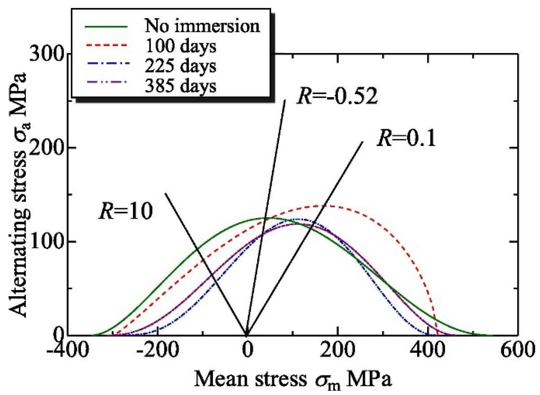
| w | Plain-woven GFRP, R = 0.1, −0.52, 10; 5 Hz; seawater | Strength degradation model; S–N and CLT diagrams—model with ageing time-dependent parameters | Koshima et al. [167] |
| T | Cross-ply, quasi-isotropic, woven FRP composites | Cumulative fatigue damage model with temperature-dependent parameters determined in constant strain rate tests | Mivehchi et al. [149] |
| T + w | GFRP UD, R = 0.1, 2; 10 Hz; fresh, sea water | Stiffness degradation model with three material parameters dependent on environmental conditions; S–N curves | Tang et al. [151] |
| T | Weave woven CFRP/epoxy laminates; R = 0.1; 20 Hz | Stiffness degradation model with damage function dependent on temperature | Khan et al. [152] |
| w | CFRP woven; 3-point bending, R = 0.1, 1 Hz; seawater | Strain-life curves with two parameters depending on samples ageing | Prabhakar et al. [145] |
| w | Epoxy resin, R = 0.1 | Viscoelastic/viscoplastic model with continuum damage accelerated by water plasticization | Rocha et al. [102] |
| T, UV | Triaxial CFRP laminates; R = −1; thermal cycles; 750 h UV | Stochastic analysis: Monte Carlo simulation for S–N curves of different guarantee areas depending on the ageing state | Mossalam et al. [137] |
| w | CFRP UD, cross-ply, bending, R = 0.1, 10 Hz, seawater | FEA modelling: virtual crack closure technique, water-induced accelerated crack propagation | Meng et al. [156] |
Publisher’s Note: MDPI stays neutral with regard to jurisdictional claims in published maps and institutional affiliations. |
© 2022 by the authors. Licensee MDPI, Basel, Switzerland. This article is an open access article distributed under the terms and conditions of the Creative Commons Attribution (CC BY) license (https://creativecommons.org/licenses/by/4.0/).
Share and Cite
Starkova, O.; Gagani, A.I.; Karl, C.W.; Rocha, I.B.C.M.; Burlakovs, J.; Krauklis, A.E. Modelling of Environmental Ageing of Polymers and Polymer Composites—Durability Prediction Methods. Polymers 2022, 14, 907. https://doi.org/10.3390/polym14050907
Starkova O, Gagani AI, Karl CW, Rocha IBCM, Burlakovs J, Krauklis AE. Modelling of Environmental Ageing of Polymers and Polymer Composites—Durability Prediction Methods. Polymers. 2022; 14(5):907. https://doi.org/10.3390/polym14050907
Chicago/Turabian StyleStarkova, Olesja, Abedin I. Gagani, Christian W. Karl, Iuri B. C. M. Rocha, Juris Burlakovs, and Andrey E. Krauklis. 2022. "Modelling of Environmental Ageing of Polymers and Polymer Composites—Durability Prediction Methods" Polymers 14, no. 5: 907. https://doi.org/10.3390/polym14050907
APA StyleStarkova, O., Gagani, A. I., Karl, C. W., Rocha, I. B. C. M., Burlakovs, J., & Krauklis, A. E. (2022). Modelling of Environmental Ageing of Polymers and Polymer Composites—Durability Prediction Methods. Polymers, 14(5), 907. https://doi.org/10.3390/polym14050907