1. Introduction
Ever-increasing special demands on structural components employ researchers in material engineering in search for material systems with exceptional properties. In particular, their mechanical and physical properties must be continuously improved to compete with the related technological progress. This also includes economical as well as ecological aspects. Textile composites appear as a suitable candidate to meet these requirements in a variety of engineering areas. Plain weave textile composites, where fibers are located in two perpendicular directions, guarantee high stiffness, strength and durability [
1] together with relatively simple manipulation when large scale composite products are prepared [
2]. Modifying the mechanical properties of the matrix by adding inorganic fillers from recycled materials [
3] may considerably improve the weight to stiffness ratio eventually leading to economically admissible designs with a sufficient bearing capacity. Exploiting green matrices would then allow us to design products which also meet the ecological requirements.
An appropriate choice of individual components opens the door for creating products with entirely unique characteristics. This calls for considerable activity in both experimental and computational research as finding an optimal material composition is not an easy task [
4]. Carbon fibers in various forms of reinforcement embedded in a polymer matrix are widely spread in constructions and products in many different branches such as aviation, shipbuilding, space industry, automotive engineering, sport equipment etc. However, the final product is generally financially demanding, which impels both manufacturers and researchers to seek for other less expensive solutions. In this regard, the basalt fibers seem to offer a promising alternative in some applications owing to their acceptable mechanical and physical properties, while considerably reducing the price of a particular product.
Basalt fibers as reinforcing material of composites have recently been exploited in the production of composites. The mechanical properties of such a composite are similar to the properties of composites reinforced with S-glass fibers and appear better than those with E-glass fiber reinforcement. Experimental results presented in [
5] showed basalt reinforced epoxy composites as a material with higher tensile, flexural and compressive Young’s modulus in comparison to E-glass fiber-based systems. The same has been observed also for compressive and bending strength, impact force and energy. Owing to better bonding between basalt fibers and epoxy resin and high interlaminar shear strength they seem to be a good option in many applications [
5,
6]. Therein, a higher stiffness in tension, flexure and compression has also been proposed for laminates. With respect to fatigue behavior, Dorigato and Pegoretti in [
7] marked the basalt fiber-based laminate as a structural element with a high capability of sustaining progressive damage. The tensile strength was found again higher than that of the glass fiber-based laminate and comparable to that of laminates reinforced with carbon fibers. When discussing the properties of basalt fiber-based composites the curing temperature is worth mentioning as this may have a great impact on the composite mechanical response [
8,
9].
Although the strength and stiffness of the composite are merely driven by the reinforcement, the overall behavior of a structural product including its durability might significantly be influenced by the choice of the matrix phase. The most common matrix material used in the production of composites is epoxy resin for its specific properties, such as hydrophobic properties, temperature, UV, and ozone resistance, and resistance to oxidation by atmospheric oxygen. Furthermore, it is inert with respect to other materials, biologically inert, non corrosive and has good electric-insulating properties [
10]. The market offers a relatively large variety of epoxy resins to serve as matrices in the production of composite materials. Among others, the L285 epoxy resin has recently been the subject of research aimed at potential improvement of its properties by adding a suitable filler [
3].
In general, the mechanical response of various epoxy resins may considerably vary. Apart from common viscoelastic or nonlinear viscoelastic behavior, one may observe a transition to brittle-viscous or even brittle response with no viscose effects [
11]. Obviously, such a different response not only influences the behavior and thus the range of applications of the corresponding composite material, but also drives the choice of the numerical method when we wish to make any predictions computationally. The geometrical complexity of the reinforcement as well as the inability to represent the overall behavior of the composite by the same constitutive model as adopted for individual components often requires a fully coupled homogenization. This is traditionally achieved with the help of FE
approach [
12]. With reference to textile composites the finite element homogenization [
13] is carried out both at the level of yarns and textile ply adopting a suitable computational model on each scale, e.g., the periodic unit cell extracted from the composite on a given scale [
14]. However, this approach might prove computationally demanding suggesting the application of more efficient methods. These fall within the category of classical micromechanical models such as the Self-consistent and Mori–Tanaka methods [
15]. The Mori–Tanaka method [
16,
17] in particular enjoys considerable attention as being fully explicit and easy to implement, see, e.g., [
18,
19,
20] for some recent applications. It also allows for a simple extension in the framework of Dvorak’s transformation field analysis [
21] to incorporate various sources of nonlinearities arising once loading the composite beyond the elastic regime.
These opening paragraphs motivated the content of the paper. The current interest in basalt fibers influenced the choice of textile reinforcements. Their potential exploitation in advanced structural elements such as wind turbine blade [
22] called for the application of high-performance synthetic epoxy resins. Expecting good physiological compatibility and superior mechanical properties the L285 epoxy resin has been found worthy of investigation. While experimental research of the resulting composite at the structural level is crucial, the initial designs are often based on numerical predictions. In light of this, an efficient computational model providing a reliable macroscopic response plays an important role. To this end, we propose a general methodology outlined within the following steps:
Identifying and calibrating a suitable constitutive model of the matrix phase.
Providing a remedy of the Mori–Tanaka (MT) micromechanical model to yield the yarn response comparable to that delivered by the finite element method (FEM). In this regard, the finite element (FE) predictions are taken as a sufficiently accurate representation of the composite response substituting the actual measurements in the framework of virtual experiments.
Developing an efficient computational scheme based on a two-scale modeling strategy where the Mori–Tanaka method is adopted as a stress updater at the level of macroscopically homogeneous yarns.
The last two items are described in detail in
Section 3 clearly identifying the novelty of this work seen in the reformulation of the original format of the Mori–Tanaka method and its application in the multi-scale computational framework of basalt babric reinforced composites.
3. Methods
The present section summarizes the theoretical background needed for a nonlinear viscoelastic modeling of plain weave textile reinforced polymer matrix composites. We begin with the formulation and calibration of the L285 epoxy resin. Essential steps to perform two-step homogenization are outlined next.
3.1. Formulation and Calibration of Generalized Leonov Model
It has been experimentally observed that polymers show, in general, a negligible volumetric strain during plastic flow. This is supported in [
32] where the application of the generalized Leonov model proved useful in the modeling of such materials. This is also why this constitutive model is exploited in the present work. As details of the model can be found in a number of contributions, see, e.g., [
33,
34], we address the theoretical grounds of the model only shortly.
The stepping stone in the formulation of the Leonov model is the Eyring flow equation representing the plastic component of the shear strain rate in the form
The total shear strain rate combining the elastic and plastic strain rates then becomes
which is the one-dimensional Leonov constitutive model [
35] with the shear-dependent viscosity
given by
where
is the shear stress and
are the model parameters,
is the viscosity corresponding to a linear viscoelastic response and
is the stress-dependent shift factor. Notice that Equation (
4) represents a single Maxwell unit with variable viscosity. To describe the material response sufficiently accurately, the generalized Maxwell chain model is typically used. Extension to multidimensional behavior introduces an equivalent deviatoric stress
as
where
s is the deviatoric stress vector. The viscosity of the
unit is then provided by
Admitting material isotropy, small strain theory, and the bulk response to be linearly elastic we arrive at the complete set of constitutive equations defining the compressible generalized Leonov model
where is the means stress, is the volumetric strain, K is the material bulk modulus, is the shear modulus, associated with the -th unit, stores the components of the deviatoric strain and .
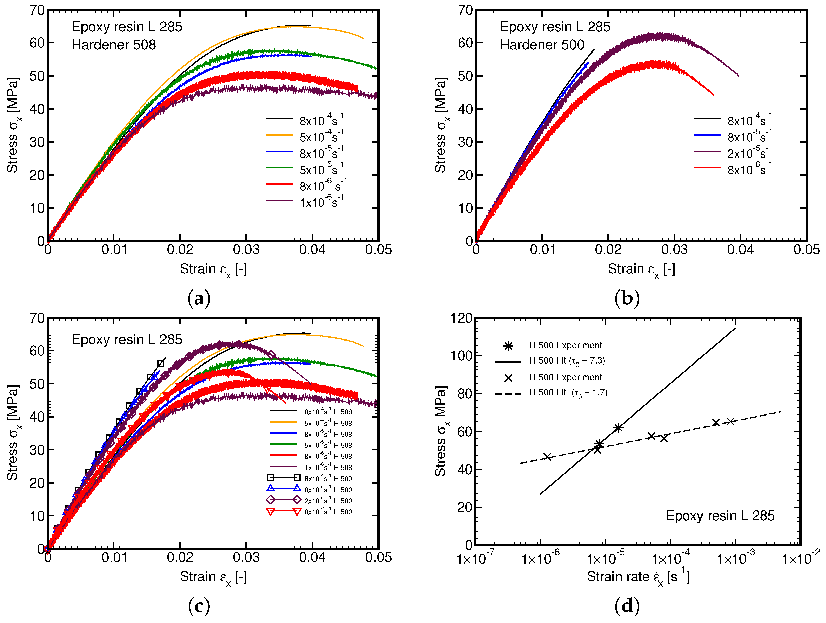
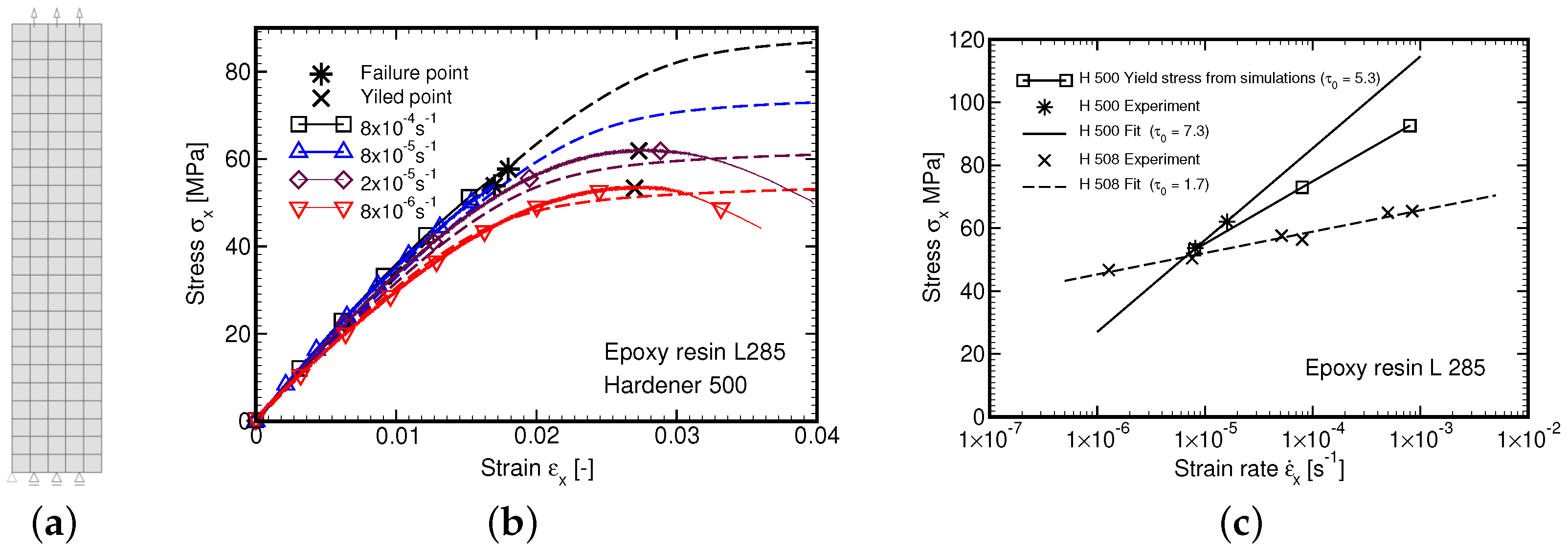
3.1.1. Tensile Tests at Different Strain Rates
The most straightforward calibration of the stress shift factor
is to construct an Eyring plot [
33,
36] assuming that at plastic yielding the plastic strain rate equals the total strain rate. The yield stress is then defined as a stress level, which remains constant at further straining. With reference to the Leonov model, we recognize the analogy with an elastic perfectly plastic von Mises material. Thus, beyond the yield point, the material behaves as a generalized Newton fluid
where the notation
was introduced for the sake of conciseness and
is the rate of equivalent deviatoric strain. In simple tension and at plastic yielding (
) we get
With reference to Equation (
3) and realizing that
is equivalent to
in plastic yielding and multidimensional space we may write
which for large values of
simplifies as
Equation (
14) thus suggests that parameters of the Eyring flow model
can be found through a linear regression in the
diagram.
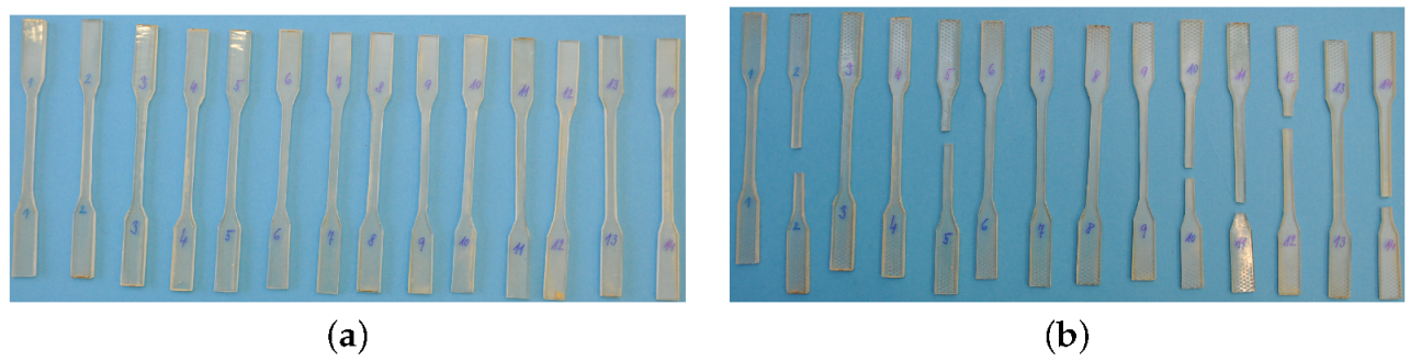
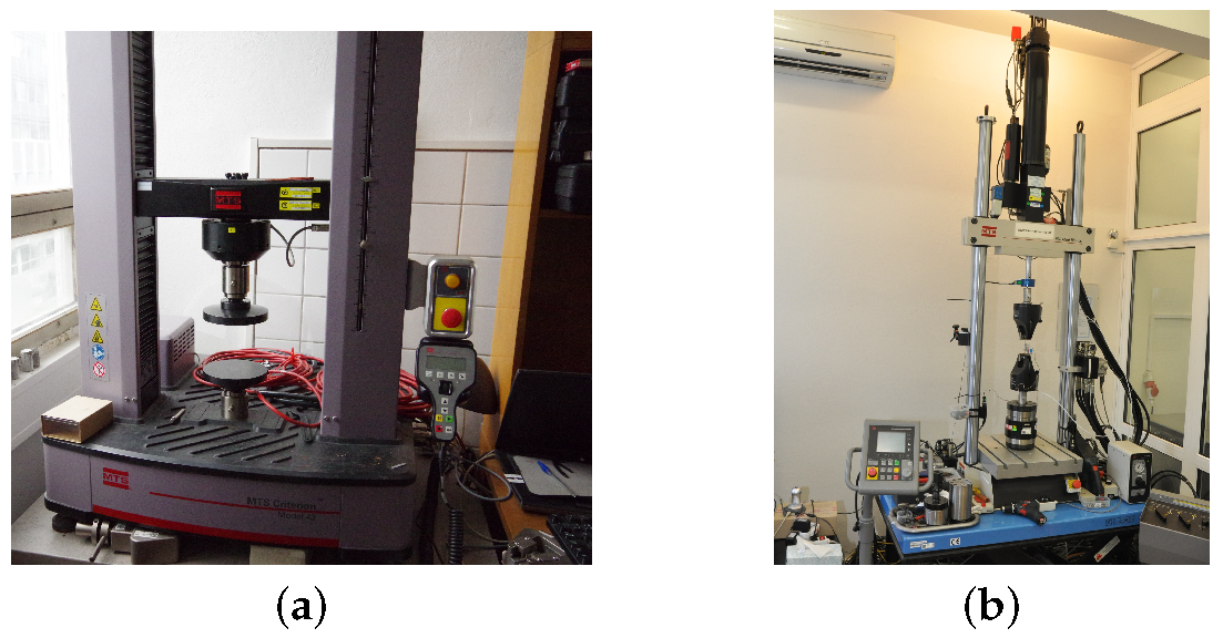
The specimens in
Figure 1 were loaded in the displacement control regime at a specific strain rate until failure using the MTS Alliance 30 kN (MTS, Eden Prairie, Minnesota, United States) electromechanical testing machine equipment with 30 kN load cell. The evolution of strain
was measured using a clip on extensometer with an initial gauge length of 25 mm tightly mounted on the surface of the tested specimen, see
Figure 5b. The corresponding stresses were derived by dividing the chamber force by the average cross-section area obtained from several measurements along the specimen length, recall
Table 2.
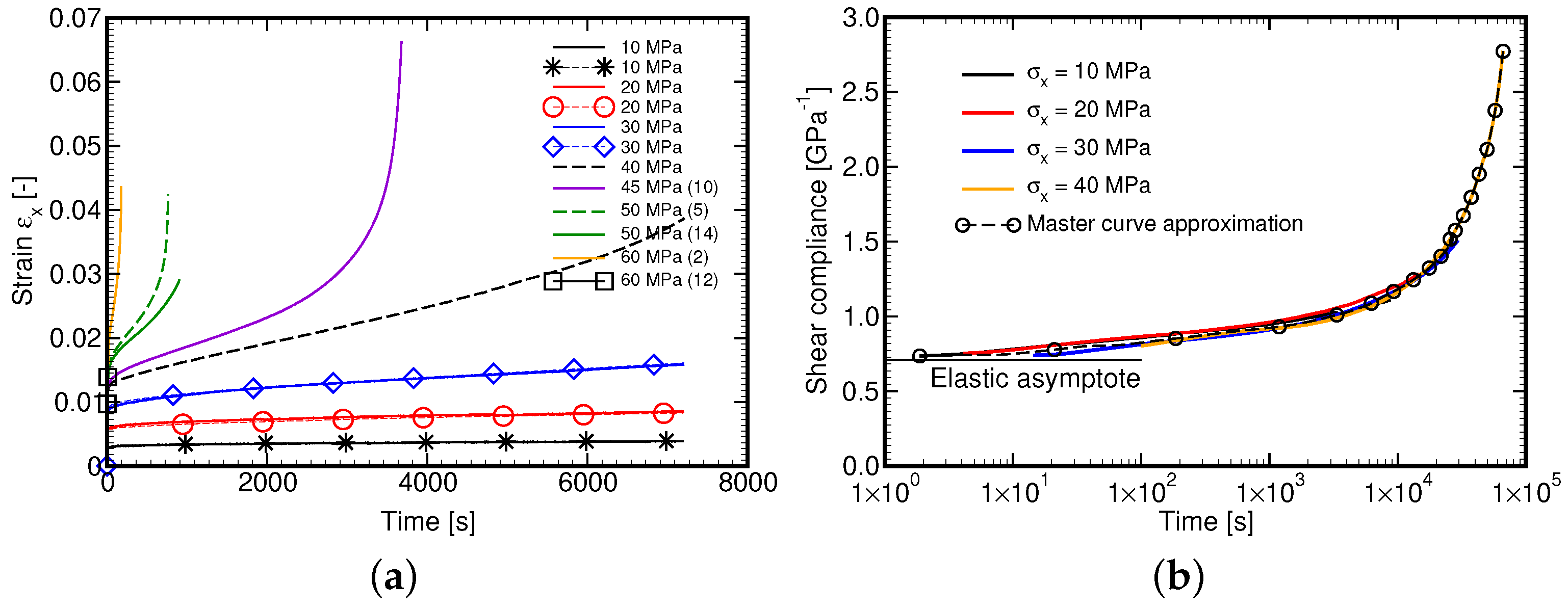
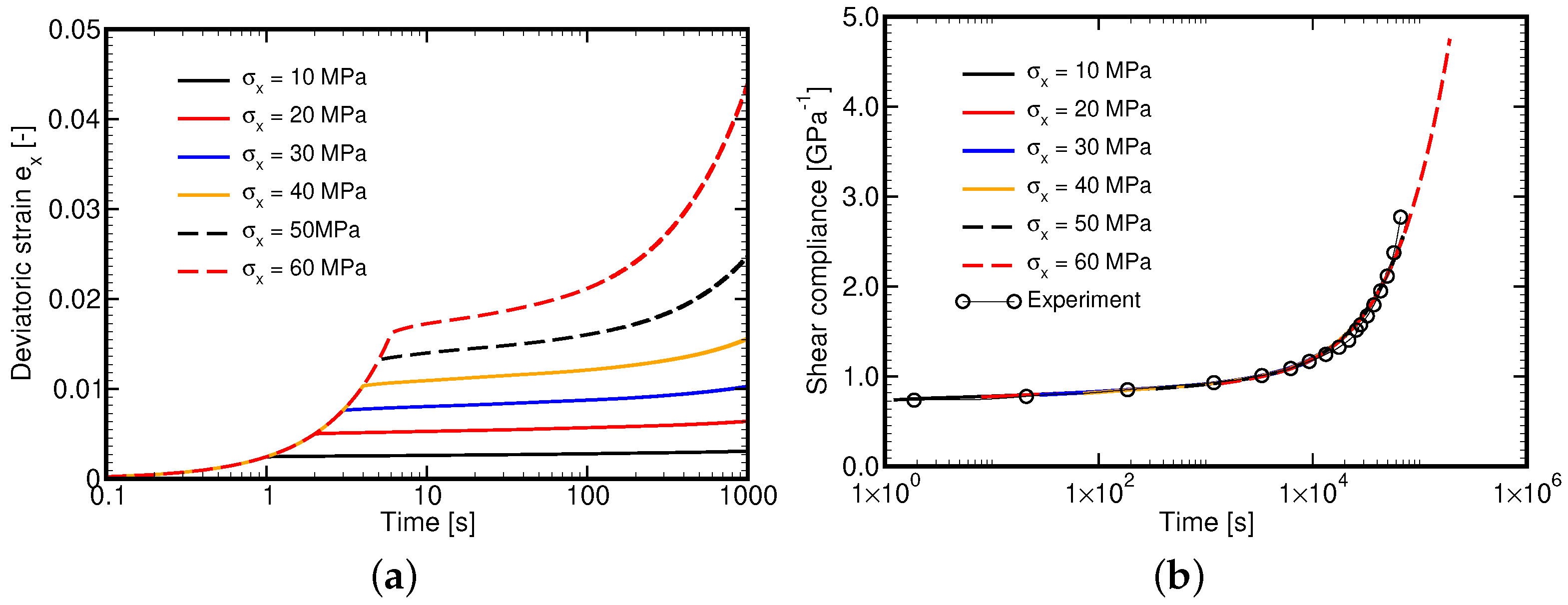
3.1.2. Creep Tests at Different Stress Levels
We open this section by assuming that the creep compliance function
can be well approximated by the Dirichlet series as
where
are the selected retardation times. Note that the first term is typically assumed sufficiently small to represent in the limit
an elastic solid. The compliances
of the Kelvin units with nonlinear viscosities
are derived by matching Equation (
15) with the experimentally derived Master curve.
The required data are provided by standard creep tests performed at different stress levels thus exploiting the time—stress superposition principle consistent with the Eyring flow model. In the present study, the MTS Mini Bionix 858.02 testing system equipped with 1000 N load cell was used, see
Figure 5b. The specimens of the same geometry as used in the tensile tests were loaded by a constant force corresponding to stresses in the range of 10 to 60 MPa. The specimen preload was carried out at a constant loading speed of 500 Ns
. The strains were then recorded for two hours using again the 25 mm gauge length extensometer. To construct the creep compliance function from the above tests we adopted the following steps:
- (1)
Transform
data into
plots where
t is the time in [s] and
is the deviatoric normal strain provided by
where
is the volumetric strain and
is the mean stress, recall Equation (8). The bulk modulus
K is calculated from the elastic modulus
E estimated from the elastic part of the stress–strain curve when preloading the specimen to the desired stress level. The Poisson ratio
is assumed to be known.
- (2)
Transform the
curves into
data where
is provided by
- (3a)
Shift the
data along the
t-axis using the corresponding shift factor
obtained previously from tensile tests, recall
Section 3.1.1. This is achieved by multiplying the original time by
. This way we arrive at the creep compliance curve (Master curve) we would obtain for a sufficiently low stress that produces a viscoelastic response and is maintained for a long time.
- (3b)
Alternatively, as will yet be proven useful, the Eyring flow model parameter
and thus the shift factor
can be estimated directly from the creep tests. To this purpose, a simple optimization algorithm was implemented in MATLAB (vr. R2021b) software. In particular, the search for
defining the shift factor
via Equation (
5) amounts to finding a minimum of a single-variable function of
on a fixed interval. When formulating the objective function to be minimized we remember that the creep compliance functions, when shifted horizontally based on a given value of
, partially overlap. In light of this, the objective function was defined as the square root of the sum of squares of deviations between the experimental data points, corresponding to consecutive load levels, over the current overlapping region. All curves were exploited at once. The minimization was performed with the help of the MATLAB function
fminbnd.
As already mentioned the search for the compliances
represents the second minimization problem written again in the framework of the least square method. To that end, we compare a certain set of experimentally measured values of the compliance function
with those provided by Equation (
15). To arrive at meaningful results, the first term in the Dirichlet series expansion
was constrained to represent the elastic limit estimated from the initial slope of the creep test. It should be mentioned that the approximation of creep compliance function using Equation (
15) is valid only for the time range specified by the retardation times
.
Application of Equation (9) calls for the transformation of creep compliance function (
15) to relaxation function
given by
Typically, the Laplace transformation is employed to obtain the relaxation times
and the shear stiffnesses
of the Maxwell units, see, e.g., [
37].
The theoretical formulation of the constitutive model of the matrix phase can be now completed by integrating Equation (9) in time. For simplicity, the most simple, those only conditionally stable, fully explicit forward Euler scheme is employed. Provided that the total strain rate is constant during the integration of a new state of stress in the matrix phase at the end of the current time step,
assumes the form
where
is the current time at the end of the
i-th time increment. In light of Equation (
18) the instantaneous shear modulus
and the increment of eigenstress
read
Further details can be found, e.g., in [
38].
3.2. Computational Homogenization
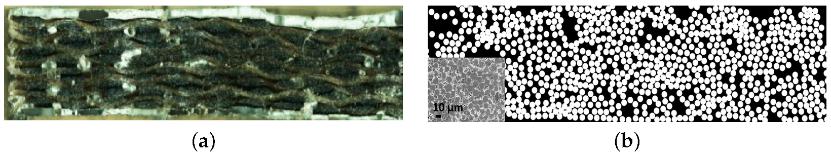
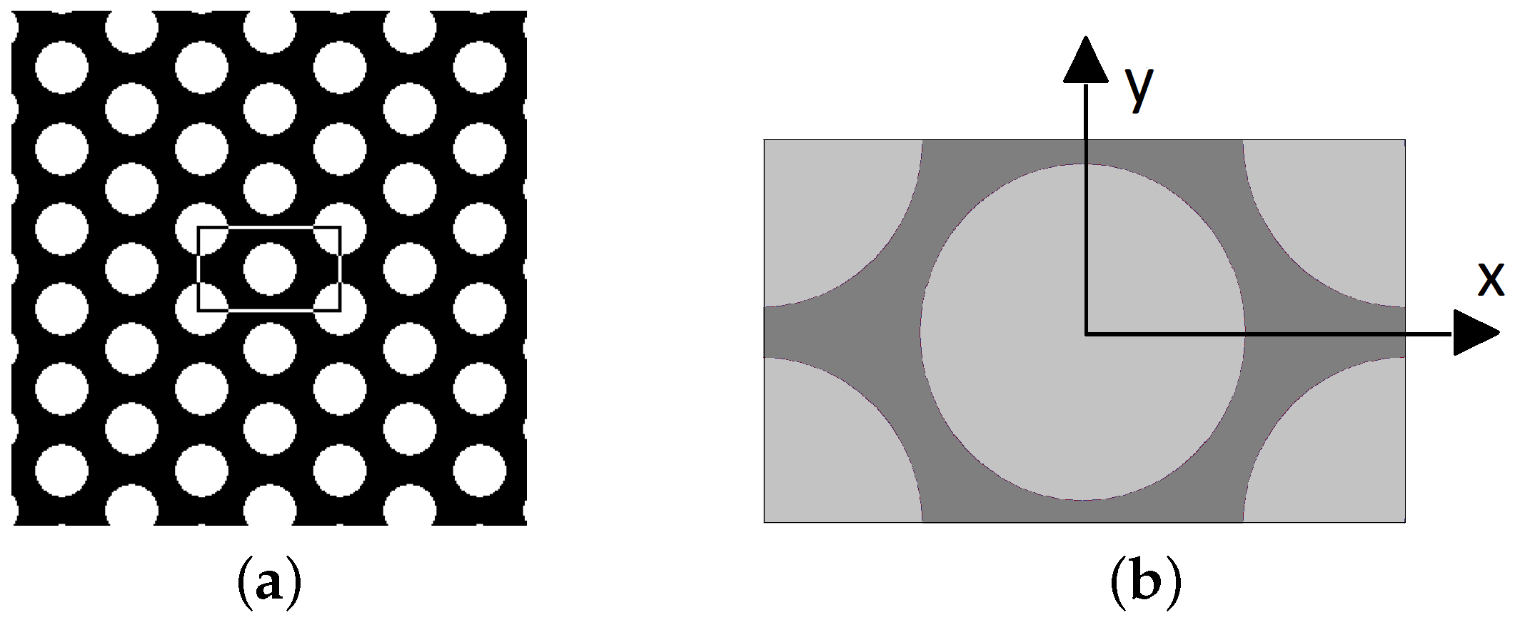
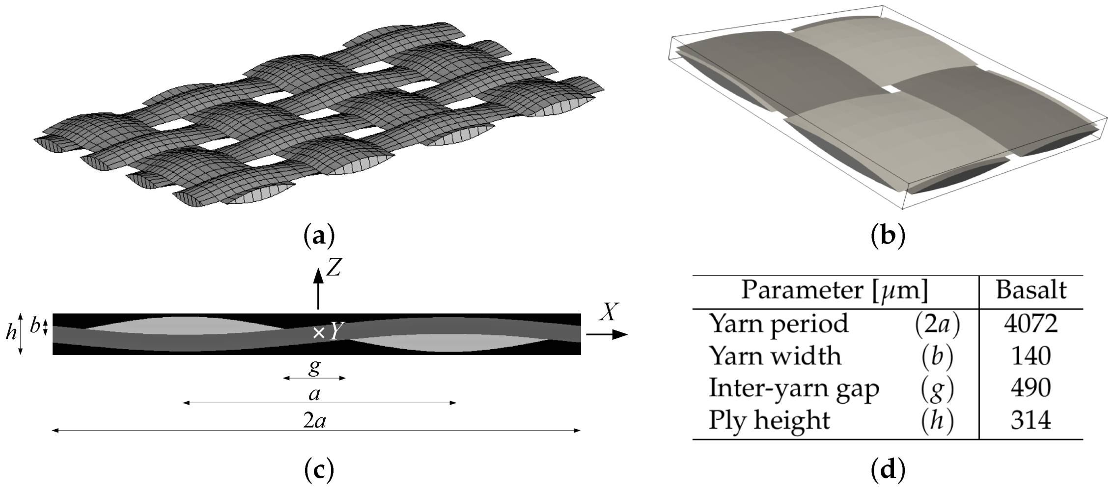
To introduce the subject we consider a representative volume element (RVE) of a single-ply balanced plain weave composite plotted in
Figure 4 with a potential distribution of fibers in the transverse cross-section being represented by a periodic hexagonal array model as plotted in
Figure 3. These simple geometrical representations allow for a standard periodic homogenization to be exploited on the mesoscopic (ply) as well as microscopic (yarn) scales.
When limiting attention to elasticity, a simple bottom-up fully uncoupled homogenization can be used to predict the macroscopic effective properties of a single-ply textile composite. This, however, is no longer possible when loading the composite beyond the elastic limits as the material anisotropy precludes derivation of the homogenized nonlinear constitute law at the level of yarn. A two-step, fully coupled homogenization, is therefore needed. Two options are typically available:
Analysis in the framework of FE
approach. In this case, the finite element homogenization is carried out both at the level of yarns and textile ply adopting a suitable computational model on each scale, e.g., the periodic unit cells in
Figure 3b and
Figure 4b. In this approach, the ply RVE (mesoscale) is typically loaded by the prescribed macroscopic strains or stresses, while the yarn RVE (microscale) is subjected to strains developed at an integration point of a finite element located in the yarn. Upon return, the updated stress averages and potentially the modified yarn effective properties are transferred back to the mesoscale.
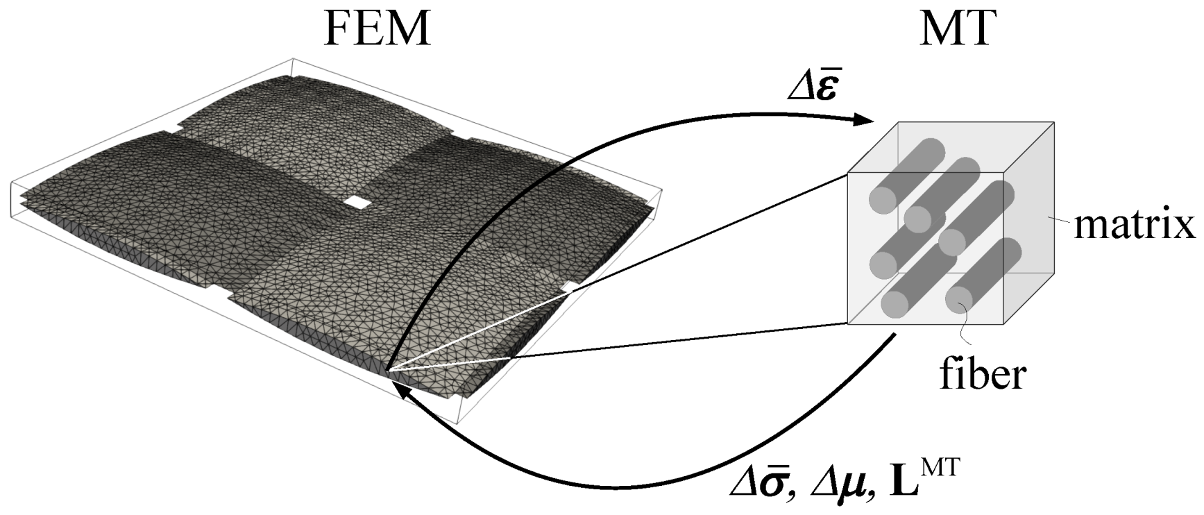
The FE
approach might be computationally too demanding. This suggests a combination of the finite element method at the level of textile ply and the computationally efficient Mori–Tanaka method which replaces the finite element analysis at the level of yarns. This approach in particular is examined in the present study. A graphical representation of this two-step modeling strategy, where
is the mesoscopic strain at a given point of the mesoscopic finite element mesh and
is the corresponding mesoscopic stress increment provided by the Mori–Tanaka method, is shown in
Figure 6. The eigenstrain
might be associated with many physical sources, but only the viscoelastic effects are considered hereinafter.
Both homogenization approaches, FE and MT method based, will be now briefly reviewed. Only the most relevant formulations will be outlined. Thus, for more details, the interested reader is referred to [
14,
15].
3.2.1. First Order Homogenization Using Finite Element Method
The presented first-order homogenization grounds on the formulation developed in [
13]. To this end, suppose that a periodic unit cell
Y, representing all the geometrical and material details of the whole composite, is loaded on its outer boundary by the prescribed displacements or tractions that produce the macroscopically uniform strains
E or stresses
in an equivalent homogeneous medium. The macroscopic constitutive equations then read
where
and
are the instantaneous effective (homogenized) stiffness and compliance matrices, respectively, and
, and
are the corresponding eigenstresses and eigenstrains. We choose an incremental format in view of the nonlinear viscoelastic model described by Equations (20)–(22). The macroscopic strains and stresses are related to volume strains and stress averages of local fields developed in individual phase
as
where
stands for volume averaging,
is the volume fraction of a given phase
r and
and
are increments of piece-wise uniform phase strains and stresses, respectively, see [
14] for further details. Similar to Equation (
23), the local fields can be written in terms of the phase material stiffness
and compliance
matrices as
where
and
are increments of local phase eigenstrains and eigenstresses. In the present study, only the viscoelastic strain
developed in the matrix will be considered.
Equation (
23) follows directly from Hill’s lemma [
39]. Hill proved that for the assumed uniform loading conditions the volume average of the internal work (virtual work) done by local fields equals the internal work (virtual work) done by their macroscopic counterparts. This statement is mathematically written as
Because in the displacement-based finite element method the primary unknowns are the nodal displacements, we continue by decomposing the local displacements, while taking into account the periodicity of the unit cell, into a homogeneous
and fluctuations
parts as
where Equation (
27)
follows from standard strain-displacement relations. Next, substituting from Equation (
27)
into Equation (
26) and realizing that
provides Hill’s lemma in the form
Because the variations
and
are independent, Equation (
29) can be split into two equalities
Equations (
30) and (31) are to be solved for unknown increments of macroscopic
and fluctuation
strain fields. When deriving this set of equations we explicitly assumed that the macroscopic stress increment
is prescribed thus considering the stress-based approach [
14]. However, the strain based formulation is often needed. In such a case, the unit cell is loaded by the prescribed macroscopic strain
. The virtual change of the prescribed quantity then vanishes (
) and Equation (
29) simplifies to
In the framework of FEM the fluctuation displacements
rather than the total displacements
u will be considered as the primary unknowns. Standard finite element discretization then reads
where matrix
stores the shape functions for a given partition of the unit cell,
is the corresponding geometrical matrix and
r is the vector of unknown nodal degrees of freedom. Introducing the fluctuation strains from Equation (
33) into Equation (
32) provides the final set of discretized equations of equilibrium in the form
where
represents the volume of the unit cell
Y. It is worth mentioning that the fluctuation displacements
must satisfy certain conditions so that the following relations hold
Point out that Equation (
35)
is for example satisfied when enforcing homogeneous displacements
r on the entire boundary of the unit cell. Usually, better predictions are obtained when considering periodic boundary conditions which for a rectangular PUC amounts to enforcing the same fluctuation displacements on opposite faces of PUC. To avoid writing any master–slave type of constraints it is preferable to consider periodic meshes. The periodicity condition is then enforced simply by assigning the same code numbers to the corresponding degrees of freedom on opposite faces of PUC.
3.2.2. Homogenization Based on Mori–Tanaka Method and Transformation Field Analysis
The Mori–Tanaka method belongs to the class of micromechanical models that ground on the Eshelby solution of an ellipsoidal inclusion problem where a single inclusion is imagined in an unbounded homogeneous body loaded at infinity by a uniform stress or strain [
40] fields. Eshelby showed that in such a case the distribution of inclusion strains and stresses is also uniform and derived a localization tensor that identifies the inclusion strain and stresses in terms of the applied far fields, material properties of the two phases and geometry of the inclusion. A number of existing micromechanical models take advantage of this result and attempt to extend the Eshelby solution to a composite with a large number of interacting inclusions. In his reformulation of the original Mori–Tanaka method [
16], Benveniste [
17] showed that the MT method accounts for the interaction of inclusions by introducing a single inclusion into an infinite matrix, but unlike the Eshelby solution this system is loaded by yet unknown average strains or stresses found in the matrix phase. This method is therefore explicit and for that reason enjoys popularity. As there is a voluminous literature on this subject, we do not attempt to present all the details of the method but provide just the relations needed in the context of this paper. To become more familiar with this method we point the interested reader to the following two monographs [
14,
15].
To be consistent with the previous section we consider again a two-phase fiber-matrix composite and write the local constitutive Equation (
25)
assuming elastic response of the fiber phase and viscoelastic response of the matrix as
where
(
, subscripts
stand for the fiber and matrix phase) is the phase material stiffness matrix and
represents the dependence on the current viscoelastic shear modulus, recall Equation (
21). The local strains in individual phases follow from the application of Dvorak’s transformation field analysis [
21] and are provided by
where
and
are the mechanical strain localization factors and strain and stress transformation influence functions, respectively. It can be shown [
15,
21] that for a two-phase composite the transformation influence functions are readily provided in terms of the localization factors as
It remains to determine the mechanical strain localization factors
. To do so, we consider, in light of the MT method, a single inclusion of an elliptical shape being embedded into an unbounded matrix, which is loaded at infinity by the average strain in the matrix phase. In the absence of viscoelastic contribution, the strain increment in the fiber phase can be then written with the help of partial strain localization factor
as
With reference to Equation (
24)
it is now possible to express the average matrix strain increment
in the form
where
is the identity matrix. Substituting the right hand side of Equation (
40) back to Equation (
39) finally gives
Without derivation, see for example [
40] for details, we provide the particular form of
, the result of the Eshelby transformation inclusion problem, as
The matrix
depends on the properties of the matrix phase and geometry of the inclusion and for the case of infinite longitudinal fibers, the only type of inclusion considered in this study, is given by [
41]
where
are the Hill moduli of the matrix phase and can be written in terms of Young’s moduli and Poisson’s ratios of transversely isotropic material, remember the material parameters of the basalt fiber listed in
Table 4, in the form
The homogenized stiffness matrix, the overall stress and eigenstress vectors associated with a lower scale, here being represented by the level of yarn (microscale), are finally provided by substituting the local stress increments from Equation (
36) into Equation (
24)
and using relations (
37) together with
to get
Comparing Equation (
44) with Equation (
23)
finally gives the homogenized stiffness matrix
and the increment of mesoscopic eigenstress
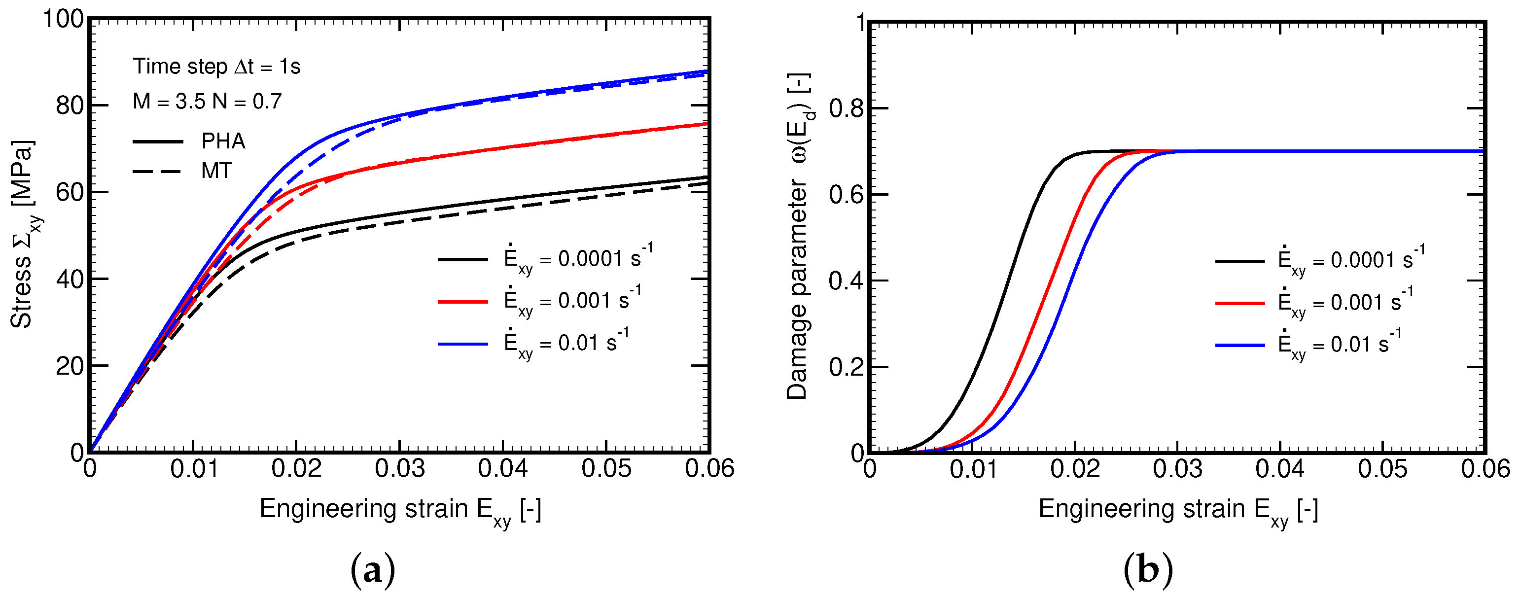
3.2.3. Modification of Original Format of Mori–Tanaka Method
The literature offers solid evidence regarding the inability of the original format of the Mori–Tanaka method (piece-wise uniform distribution of strains and stresses in individual phases) to provide results comparable to detailed numerical simulations using FEM for loading conditions exceeding the elastic limit, see [
42,
43,
44] (for illustration).
A much stiffer response predicted by the MT method is typically observed. This can be attributed to the way the stresses are localized into the fiber phase as the matrix response is assumed to be controlled solely by the constitutive law. In FEM simulations the stress transfer between individual phases is most probably affected by the formation of shear bands in the matrix. Here, we attempt to address this issue by suitably modifying the local constitutive model of the fiber phase. Being inspired by [
45,
46] we suggest to reduce the stresses taken by the fibers through a damage-like parameter
and write the fiber stress increment as
where
represent the deviatoric and mean components of the fiber stress increment
, respectively. The tensorial notation in Equations (48) and (49) is adopted just for the sake of convenience. Point out that stress reduction applies to the deviatoric stress components only.
The evolution of damage parameter
is assumed similar to that proposed in [
46] but replaces the equivalent stress
with the viscoelastic equivalent deviatoric strain in the matrix
. Considering only the viscoelastic part of the total strain allows us to write
where
are the model parameters. These parameters are found by matching the FEM predictions of the homogenized response by comparing the PHA model predictions and the MT two-phase estimates given by Equation (
44). Note that the stiffness matrix of the fiber phase
must be suitably modified by introducing a reduced shear modulus
The scaling parameter
is written in terms of
and the elastic shear modulus
, recall Equation (
1), as
5. Conclusions
Since gaining notable popularity, the basalt fabric/polymer matrix based composites should be thoroughly studied both experimentally and computationally, for only then new improved designs would be broadly accepted in structural applications. The present study partially contributes to this subject by offering an efficient fully coupled two-scale computational procedure to address both the geometrical complexity of basalt reinforcement and nonlinear behavior of the matrix.
The proposed approach advocates the use of the Mori–Tanaka micromechanical model to substitute a computationally expensive finite element method when estimating local stresses and strains on the yarn scale. The fact that only the overall macroscopic response is usually of an engineering interest supports this approach as the MT method generally obviates the local details by considering the piece-wise uniform stress and strain averages only. However, even such a simplification should be reliable and generally comparable to more accurate FE predictions. This is why we introduced a certain reformulation of the original format of the MT method to closely match the mesoscopic response generated by FEM. In this context, the presented results seem promising so to accept the MT method for the stress update on the microscale (unidirectional fibrous composite representing yarn) within the multiscale analysis. In this regard, some specific features of the macroscopic response of a textile ply with reference to the adopted local constitutive laws have successfully been illustrated.
While this study is only computational and should be experimentally validated, the analysis concerning the material behavior of individual phases, the basalt fibers and L285 polymer matrix, integrated both experimental and computational components of research. A complex experimental program was executed to provide data for the calibration of the generalized Leonov model chosen to represent the nonlinear viscoelastic response of the matrix phase. Within this step, a calibration procedure for tuning the model parameters of the Eyring flow was developed solely on the basis of creep tests. The calibrated model was validated computationally by reproducing the laboratory measurements numerically. The reported results highlight the importance of properly addressing the whole system resin/hardener as the results derived for one particular hardener can hardly be transplanted to another one albeit using the same epoxy resin.


 ,
, 


